EXPLAINABLE DEEP ONE-CLASS CLASSIFICATION
←
→
Page content transcription
If your browser does not render page correctly, please read the page content below
Published as a conference paper at ICLR 2021

E XPLAINABLE D EEP O NE -C LASS C LASSIFICATION
 Philipp Liznerski1∗       Lukas Ruff2∗        Robert A. Vandermeulen2∗
                  1                      1
 Billy Joe Franks         Marius Kloft         Klaus-Robert Müller2 3 4 5
 1
   ML group, Technical University of Kaiserslautern, Germany
 2
   ML group, Technical University of Berlin, Germany
 3
   Google Research, Brain Team, Berlin, Germany
 4
   Department of Artificial Intelligence, Korea University, Seoul, Republic of Korea
 5
   Max Planck Institute for Informatics, Saarbrücken, Germany
 {liznerski, franks, kloft}@cs.uni-kl.de
 {lukas.ruff, vandermeulen, klaus-robert.mueller}@tu-berlin.de

                                               A BSTRACT
            Deep one-class classification variants for anomaly detection learn a mapping that
            concentrates nominal samples in feature space causing anomalies to be mapped
            away. Because this transformation is highly non-linear, finding interpretations poses
            a significant challenge. In this paper we present an explainable deep one-class
            classification method, Fully Convolutional Data Description (FCDD), where the
            mapped samples are themselves also an explanation heatmap. FCDD yields com-
            petitive detection performance and provides reasonable explanations on common
            anomaly detection benchmarks with CIFAR-10 and ImageNet. On MVTec-AD,
            a recent manufacturing dataset offering ground-truth anomaly maps, FCDD sets
            a new state of the art in the unsupervised setting. Our method can incorporate
            ground-truth anomaly explanations during training and using even a few of these
            (∼ 5) improves performance significantly. Finally, using FCDD’s explanations, we
            demonstrate the vulnerability of deep one-class classification models to spurious
            image features such as image watermarks.1

1       I NTRODUCTION
Anomaly detection (AD) is the task of identifying anomalies in a corpus of data (Edgeworth, 1887;
Barnett and Lewis, 1994; Chandola et al., 2009; Ruff et al., 2021). Powerful new anomaly detectors
based on deep learning have made AD more effective and scalable to large, complex datasets such as
high-resolution images (Ruff et al., 2018; Bergmann et al., 2019). While there exists much recent
work on deep AD, there is limited work on making such techniques explainable. Explanations are
needed in industrial applications to meet safety and security requirements (Berkenkamp et al., 2017;
Katz et al., 2017; Samek et al., 2020), avoid unfair social biases (Gupta et al., 2018), and support
human experts in decision making (Jarrahi, 2018; Montavon et al., 2018; Samek et al., 2020). One
typically makes anomaly detection explainable by annotating pixels with an anomaly score and, in
some applications, such as finding tumors in cancer detection (Quellec et al., 2016), these annotations
are the primary goal of the detector.
One approach to deep AD, known as Deep Support Vector Data Description (DSVDD) (Ruff
et al., 2018), is based on finding a neural network that transforms data such that nominal data is
concentrated to a predetermined center and anomalous data lies elsewhere. In this paper we present
Fully Convolutional Data Description (FCDD), a modification of DSVDD so that the transformed
samples are themselves an image corresponding to a downsampled anomaly heatmap. The pixels in
this heatmap that are far from the center correspond to anomalous regions in the input image. FCDD
does this by only using convolutional and pooling layers, thereby limiting the receptive field of each
output pixel. Our method is based on the one-class classification paradigm (Moya et al., 1993; Tax,
2001; Tax and Duin, 2004; Ruff et al., 2018), which is able to naturally incorporate known anomalies
Ruff et al. (2021), but is also effective when simply using synthetic anomalies.
    ∗
        equal contribution
    1
        Our code is available at: https://github.com/liznerski/fcdd

                                                     1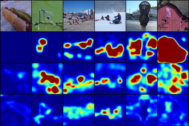
Published as a conference paper at ICLR 2021
We show that FCDD’s anomaly detection performance is close to the state of the art on the standard
AD benchmarks with CIFAR-10 and ImageNet while providing transparent explanations. On MVTec-
AD, an AD dataset containing ground-truth anomaly maps, we demonstrate the accuracy of FCDD’s
explanations (see Figure 1), where FCDD sets a new state of the art. In further experiments we
find that deep one-class classification models (e.g. DSVDD) are prone to the “Clever Hans” effect
(Lapuschkin et al., 2019) where a detector fixates on spurious features such as image watermarks. In
general, we find that the generated anomaly heatmaps are less noisy and provide more structure than
the baselines, including gradient-based methods (Simonyan et al., 2013; Sundararajan et al., 2017)
and autoencoders (Sakurada and Yairi, 2014; Bergmann et al., 2019).
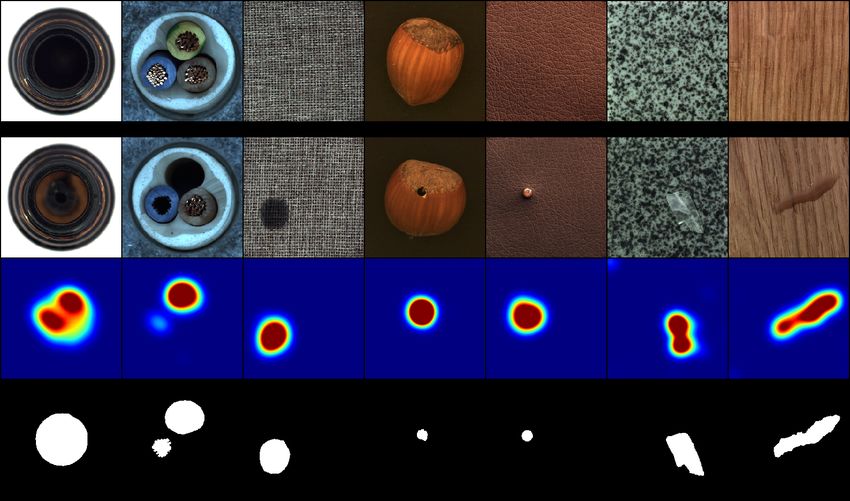
Figure 1: FCDD explanation heatmaps for MVTec-AD (Bergmann et al., 2019). Rows from top
to bottom show: (1) nominal samples (2) anomalous samples (3) FCDD anomaly heatmaps (4)
ground-truth anomaly maps.
2 R ELATED W ORK
Here we outline related works on deep AD focusing on explanation approaches. Classically deep
AD used autoencoders (Hawkins et al., 2002; Sakurada and Yairi, 2014; Zhou and Paffenroth, 2017;
Zhao et al., 2017). Trained on a nominal dataset autoencoders are assumed to reconstruct anomalous
samples poorly. Thus, the reconstruction error can be used as an anomaly score and the pixel-wise
difference as an explanation (Bergmann et al., 2019), thereby naturally providing an anomaly heatmap.
Recent works have incorporated attention into reconstruction models that can be used as explanations
(Venkataramanan et al., 2019; Liu et al., 2020). In the domain of videos, Sabokrou et al. (2018) used
a pre-trained fully convolutional architecture in combination with a sparse autoencoder to extract
2D features and provide bounding boxes for anomaly localization. One drawback of reconstruction
methods is that they offer no natural way to incorporate known anomalies during training.
More recently, one-class classification methods for deep AD have been proposed. These methods
attempt to separate nominal samples from anomalies in an unsupervised manner by concentrating
nominal data in feature space while mapping anomalies to distant locations (Ruff et al., 2018;
Chalapathy et al., 2018; Goyal et al., 2020). In the domain of NLP, DSVDD has been successfully
applied to text, which yields a form of interpretation using attention mechanisms (Ruff et al., 2019).
For images, Kauffmann et al. (2020) have used a deep Taylor decomposition (Montavon et al., 2017)
to derive relevance scores.
Some of the best performing deep AD methods are based on self-supervision. These methods
transform nominal samples, train a network to predict which transformation was used on the input, and
2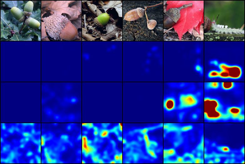
Published as a conference paper at ICLR 2021

provide an anomaly score via the confidence of the prediction (Golan and El-Yaniv, 2018; Hendrycks
et al., 2019b). Hendrycks et al. (2019a) have extended this to incorporate known anomalies as well.
No explanation approaches have been considered for these methods so far.
Finally, there exists a great variety of explanation methods in general, for example model-agnostic
methods (e.g. LIME (Ribeiro et al., 2016)) or gradient-based techniques (Simonyan et al., 2013;
Sundararajan et al., 2017). Relating to our work, we note that fully convolutional architectures have
been used for supervised segmentation tasks where target segmentation maps are required during
training (Long et al., 2015; Noh et al., 2015).

3    E XPLAINING D EEP O NE -C LASS C LASSIFICATION
We review one-class classification and fully convolutional architectures before presenting our method.

Deep One-Class Classification Deep one-class classification (Ruff et al., 2018; 2020b) performs
anomaly detection by learning a neural network to map nominal samples near a center c in output
space, causing anomalies to be mapped away. For our method we use a Hypersphere Classifier
(HSC) (Ruff et al., 2020a), a recently proposed modification of Deep SAD (Ruff et al., 2020b),
a semi-supervised version of DSVDD (Ruff et al., 2018). Let X1 , . . . , Xn denote a collection of
samples and y1 , . . . , yn be labels where yi = 1 denotes an anomaly and yi = 0 denotes a nominal
sample. Then the HSC objective is
                    n
                 1X
         min           (1 − yi )h(φ(Xi ; W) − c) − yi log (1 − exp (−h(φ(Xi ; W) − c))) ,            (1)
         W,c     n i=1

where c ∈ Rd is the center, and φ : Rc×h×w → Rd aq        neural network with weights W. Here h is
                                                                2
the pseudo-Huber loss (Huber et al., 1964), h(a) = kak2 + 1 − 1, which is a robust loss that
interpolates from quadratic to linear penalization. The HSC loss encourages φ to map nominal
samples near c and anomalous samples away from the center c. In our implementation, the center c
corresponds to the bias term in the last layer of our networks, i.e. is included in the network φ, which
is why we omit c in the FCDD objective below.

Fully Convolutional Architecture Our
method uses a fully convolutional network
(FCN) (Long et al., 2015; Noh et al., 2015)
that maps an image to a matrix of features,
i.e. φ : Rc×h×w → R1×u×v by using al-
ternating convolutional and pooling layers
only, and does not contain any fully con-
nected layers. In this context, pooling can Figure 2: Visualization of a 3×3 convolution followed
be seen as a special kind of convolution by a 3×3 transposed convolution with a Gaussian kernel,
with fixed parameters.                      both using a stride of 2.
A core property of a convolutional layer is that each pixel of its output only depends on a small region
of its input, known as the output pixel’s receptive field. Since the output of a convolution is produced
by moving a filter over the input image, each output pixel has the same relative position as its
associated receptive field in the input. For instance, the lower-left corner of the output representation
has a corresponding receptive field in the lower-left corner of the input image, etc. (see Figure 2
left side). The outcome of several stacked convolutions also has receptive fields of limited size and
consistent relative position, though their size grows with the amount of layers. Because of this an
FCN preserves spatial information.

Fully Convolutional Data Description Here we introduce our novel explainable AD method Fully
Convolutional Data Description (FCDD). By taking advantage of FCNs along with the HSC above,
we propose a deep one-class method where the output features preserve spatial information and
also serve as a downsampled anomaly heatmap. For situations where one would like to have a
full-resolution heatmap, we include a methodology for upsampling the low-resolution heatmap based
on properties of receptive fields.

                                                   3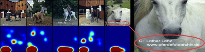
Published as a conference paper at ICLR 2021

     X

                                        Φ                                                  A‘

                                                                    A

                    FCDD

                                                                Upsamp
                                                                      ling

Figure 3: Visualization of the overall procedure to produce full-resolution anomaly heatmaps with
FCDD. X denotes the input, φ the network, A the produced anomaly heatmap and A0 the upsampled
version of A using a transposed Gaussian convolution.

FCDD is trained using samples that are labeled as nominal or anomalous. As before, let X1 , . . . , Xn
denote a collection of samples with labels y1 , . . . , yn where yi = 1 denotes an anomaly and yi = 0
denotes a nominal sample. Anomalous samples can simply be a collection of random images which
are not from the nominal collection, e.g. one of the many large collections of images which are freely
available like 80 Million Tiny Images (Torralba et al., 2008) or ImageNet (Deng et al., 2009). The
use of such an auxiliary corpus has been recommended in recent works on deep AD, where it is
termed Outlier Exposure (OE) (Hendrycks et al., 2019a;b). When one has access to “true” examples
of the anomalous dataset, i.e. something that is likely to be representative of what will be seen
at test time, we find that even using a few examples as the corpus of labeled anomalies performs
exceptionally well. Furthermore, in the absence of any sort of known anomalies, one can generate
synthetic anomalies, which we find is also very effective.
With an FCN φ : Rc×h×wp→ R
                               u×v
                                    the FCDDobjective utilizes a pseudo-Huber loss on the FCN
output matrix A(X) =                2
                          φ(X; W) + 1 − 1 , where all operations are applied element-wise. The
FCDD objective is then defined as (cf., (1)):

                    n
                 1X               1                                1
         min           (1 − yi )     kA(Xi )k1 − yi log 1 − exp −     kA(Xi )k1    .                (2)
          W      n i=1           u·v                              u·v

Here kA(X)k1 is the sum of all entries in A(X), which are all positive. FCDD is the utilization of
an FCN in conjunction with the novel adaptation of the HSC loss we propose in (2). The objective
maximizes kA(X)k1 for anomalies and minimizes it for nominal samples, thus we use kA(X)k1 as
the anomaly score. Entries of A(X) that contribute to kA(X)k1 correspond to regions of the input
image that add to the anomaly score. The shape of these regions depends on the receptive field of the
FCN. We include a sensitivity analysis on the size of the receptive field in Appendix A, where we
find that performance is not strongly affected by the receptive field size. Note that A(X) has spatial
dimensions u × v and is smaller than the original image dimensions h × w. One could use A(X)
directly as a low-resolution heatmap of the image, however it is often desirable to have full-resolution
heatmaps. Because we generally lack ground-truth anomaly maps in an AD setting during training, it
is not possible to train an FCN in a supervised way to upsample the low-resolution heatmap A(X)
(e.g. as in (Noh et al., 2015)). For this reason we introduce an upsampling scheme based on the
properties of receptive fields.

                                                   4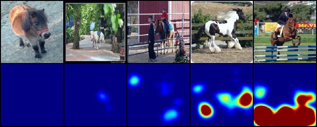
Published as a conference paper at ICLR 2021

Heatmap Upsampling Since we gener-
                                               Algorithm 1 Receptive Field Upsampling
ally do not have access to ground-truth                      u×v
pixel annotations in anomaly detection dur- Input: A ∈ R           (low-res anomaly heatmap)
                                                           0     h×w
ing training, we cannot learn how to upsam- Output: A ∈ R              (full-res anomaly
                                                                                      heatmap)
ple using a deconvolutional type of struc- Define: [G2 (µ, σ)]x,y , 1 2 exp − (x−µ1 )2 +(y−µ      2)
                                                                                                    2

                                                                           2πσ               2σ 2
ture. We derive a principled way to upsam-
ple our lower resolution anomaly heatmap         A0 ← 0
instead. For every output pixel in A(X)          for all output pixels a in A do
there is a unique input pixel which lies at          f ← receptive field of a
the center of its receptive field. It has been       c ← center of field f
observed before that the effect of the recep-        A0 ← A0 + a · G2 (c, σ)
tive field for an output pixel decays in a       end for
Gaussian manner as one moves away from           return A0
the center of the receptive field (Luo et al.,
2016). We use this fact to upsample A(X) by using a strided transposed convolution with a fixed
Gaussian kernel (see Figure 2 right side). We describe this operation and procedure in Algorithm 1
which simply corresponds to a strided transposed convolution. The kernel size is set to the receptive
field range of FCDD and the stride to the cumulative stride of FCDD. The variance of the distribution
can be picked empirically (see Appendix B for details). Figure 3 shows a complete overview of our
FCDD method and the process of generating full-resolution anomaly heatmaps.

4     E XPERIMENTS

In this section, we experimentally evaluate the performance of FCDD both quantitatively and
qualitatively. For a quantitative evaluation, we use the Area Under the ROC Curve (AUC) (Spackman,
1989) which is the commonly used measure in AD. For a qualitative evaluation, we compare the
heatmaps produced by FCDD to existing deep AD explanation methods. As baselines, we consider
gradient-based methods (Simonyan et al., 2013) applied to hypersphere classifier (HSC) models (Ruff
et al., 2020a) with unrestricted network architectures (i.e. networks that also have fully connected
layers) and autoencoders (Bergmann et al., 2019) where we directly use the pixel-wise reconstruction
error as an explanation heatmap. We slightly blur the heatmaps of the baselines with the same
Gaussian kernel we use for FCDD, which we found results in less noisy, more interpretable heatmaps.
We include heatmaps without blurring in Appendix G. We adjust the contrast of the heatmaps per
method to highlight interesting features; see Appendix C for details. For our experiments we don’t
consider model-agnostic explanations, such as LIME (Ribeiro et al., 2016) or anchors (Ribeiro et al.,
2018), because they are not tailored to the AD task and performed poorly.

4.1   S TANDARD A NOMALY D ETECTION B ENCHMARKS

We first evaluate FCDD on the Fashion-MNIST, CIFAR-10, and ImageNet datasets. The common
AD benchmark is to utilize these classification datasets in a one-vs-rest setup where the “one” class is
used as the nominal class and the rest of the classes are used as anomalies at test time. For training,
we only use nominal samples as well as random samples from some auxiliary Outlier Exposure (OE)
(Hendrycks et al., 2019a) dataset, which is separate from the ground-truth anomaly classes following
Hendrycks et al. (2019a;b). We report the mean AUC over all classes for each dataset.

Fashion-MNIST We consider each of the ten Fashion-MNIST (Xiao et al., 2017) classes in a
one-vs-rest setup. We train Fashion-MNIST using EMNIST (Cohen et al., 2017) or grayscaled
CIFAR-100 (Krizhevsky et al., 2009) as OE. We found that the latter slightly outperforms the former
(∼3 AUC percent points). On Fashion-MNIST, we use a network that consists of three convolutional
layers with batch normalization, separated by two downsampling pooling layers.

CIFAR-10 We consider each of the ten CIFAR-10 (Krizhevsky et al., 2009) classes in a one-vs-rest
setup. As OE we use CIFAR-100, which does not share any classes with CIFAR-10. We use a model
similar to LeNet-5 (LeCun et al., 1998), but decrease the kernel size to three, add batch normalization,
and replace the fully connected layers and last max-pool layer with two further convolutions.

                                                   5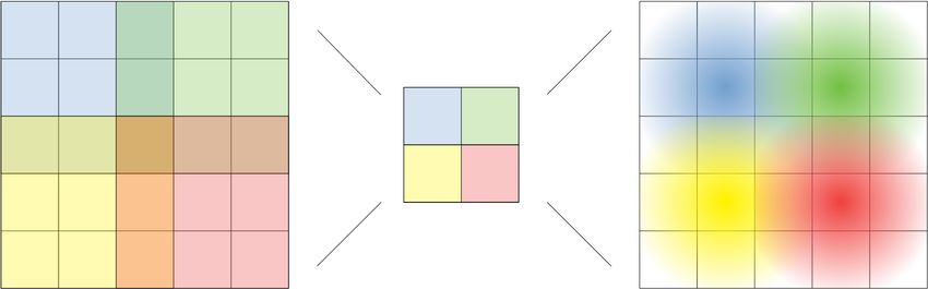
Published as a conference paper at ICLR 2021

ImageNet We consider 30 classes from ImageNet1k (Deng et al., 2009) for the one-vs-rest setup
following Hendrycks et al. (2019a). For OE we use ImageNet22k with ImageNet1k classes removed
(Hendrycks et al., 2019a). We use an adaptation of VGG11 (Simonyan and Zisserman, 2015) with
batch normalization, suitable for inputs resized to 224×224 (see Appendix D for model details).

State-of-the-art Methods We report results from state-of-the-art deep anomaly detection methods.
Methods that do not incorporate known anomalies are the autoencoder (AE), DSVDD (Ruff et al.,
2018), Geometric Transformation based AD (GEO) (Golan and El-Yaniv, 2018), and a variant of GEO
by Hendrycks et al. (2019b) (GEO+). Methods that use OE are a Focal loss classifier (Hendrycks
et al., 2019b), also GEO+, Deep SAD (Ruff et al., 2020b), and HSC (Ruff et al., 2020a).

Table 1: Mean AUC (over all classes and 5 seeds per class) for Fashion-MNIST, CIFAR-10, and
ImageNet. Results from existing literature are marked with an asterisk (Bergman and Hoshen, 2020;
Golan and El-Yaniv, 2018; Hendrycks et al., 2019b; Ruff et al., 2020a).

                               without OE                                  with OE
 Dataset             AE     DSVDD* GEO*          Geo+*   Focal*   Geo+*   Deep SAD*   HSC*    FCDD
 Fashion-MNIST      0.82     0.93         0.94    ×        ×       ×         ×          ×      0.89
 CIFAR-10           0.59*    0.65         0.86   0.90     0.87    0.96      0.95       0.96    0.95
 ImageNet           0.56      ×            ×      ×       0.56    0.86      0.97       0.97    0.94

Quantitative Results The mean AUC detection performance on the three AD benchmarks are
reported in Table 1. We can see that FCDD, despite using a restricted FCN architecture to improve
explainability, achieves a performance that is close to state-of-the-art methods and outperforms
autoencoders, which yield a detection performance close to random on more complex datasets. We
provide detailed results for all individual classes in Appendix F.
            Input
            Ours
            Grad
            AE

  (a)                               (b)                                       (c)

Figure 4: Anomaly heatmaps for anomalous test samples of a Fashion-MNIST model trained on
nominal class “trousers” (nominal samples are shown in (a)). In (b) CIFAR-100 was used for OE and
in (c) EMNIST. Columns are ordered by increasing anomaly score from left to right, i.e. what FCDD
finds the most nominal looking anomaly on the left to the most anomalous looking anomaly on the
right.

Qualitative Results Figures 4 and 5 show the heatmaps for Fashion-MNIST and ImageNet respec-
tively. For a Fashion-MNIST model trained on the nominal class “trousers,” the heatmaps show
that FCDD correctly highlights horizontal elements as being anomalous, which makes sense since
trousers are vertically aligned. For an ImageNet model trained on the nominal class “acorns,” we
observe that colors seem to be fairly relevant features with green and brown areas tending to be seen
as more nominal, and other colors being deemed anomalous, for example the red barn or the white
snow. Nonetheless, the method also seems capable of using more semantic features, for example
it recognizes the green caterpillar as being anomalous and it distinguishes the acorn to be nominal
despite being against a red background.
Figure 6 shows heatmaps for CIFAR-10 models with varying amount of OE, all trained on the nominal
class “airplane.” We can see that, as the number of OE samples increases, FCDD tends to concentrate

                                                   6
Published as a conference paper at ICLR 2021
Input
Ours
Grad
AE
(a) (b)
Figure 5: Anomaly heatmaps of an ImageNet model trained on nominal class “acorns.” Here (a) are
nominal samples and (b) are anomalous samples. Columns are ordered by increasing anomaly score
from left to right, i.e. what FCDD finds the most nominal looking on the left to the most anomalous
looking on the right for (a) nominal samples and (b) anomalies.
the explanations more on the primary object in the image, i.e. the bird, ship, and truck. We provide
further heatmaps for additional classes from all datasets in Appendix G.
Input Ours Grad AE
Figure 6: Anomaly heatmaps for three anomalous test samples on a CIFAR-10 model trained on
nominal class “airplane.” The second, third, and fourth blocks show the heatmaps of FCDD, gradient-
based heatmaps of HSC, and AE heatmaps respectively. For Ours and Grad, we grow the number of
OE samples from 2, 8, 128, 2048 to full OE. AE is not able to incorporate OE.
Baseline Explanations We found the gradient-based heatmaps to mostly produce centered blobs
which lack spatial context (see Figure 6) and thus are not useful for explaining. The AE heatmaps,
being directly tied to the reconstruction error anomaly score, look reasonable. We again note, however,
that it is not straightforward how to include auxiliary OE samples or labeled anomalies into an AE
approach, which leaves them with a poorer detection performance (see Table 1). Overall we find that
the proposed FCDD anomaly heatmaps yield a good and consistent visual interpretation.
4.2 E XPLAINING D EFECTS IN M ANUFACTURING
Here we compare the performance of FCDD on the MVTec-AD dataset of defects in manufacturing
(Bergmann et al., 2019). This datasets offers annotated ground-truth anomaly segmentation maps
for testing, thus allowing a quantitative evaluation of model explanations. MVTec-AD contains 15
object classes of high-resolution RGB images with up to 1024×1024 pixels, where anomalous test
samples are further categorized in up to 8 defect types, depending on the class. We follow Bergmann
et al. (2019) and compute an AUC from the heatmap pixel scores, using the given (binary) anomaly
segmentation maps as ground-truth pixel labels. We then report the mean over all samples of this
“explanation” AUC for a quantitative evaluation. For FCDD, we use a network that is based on a
VGG11 network pre-trained on ImageNet, where we freeze the first ten layers, followed by additional
fully convolutional layers that we train.
7Published as a conference paper at ICLR 2021
Synthetic Anomalies OE with a natural image dataset like ImageNet
is not informative for MVTec-AD since anomalies here are subtle defects
of the nominal class, rather than being out of class (see Figure 1). For this
reason, we generate synthetic anomalies using a sort of “confetti noise,”
a simple noise model that inserts colored blobs into images and reflects
the local nature of anomalies. See Figure 7 for an example. Figure 7: Confetti noise.
Semi-Supervised FCDD A major advantage of FCDD in comparison to reconstruction-based
methods is that it can be readily used in a semi-supervised AD setting (Ruff et al., 2020b). To see the
effect of having even only a few labeled anomalies and their corresponding ground-truth anomaly
maps available for training, we pick for each MVTec-AD class just one true anomalous sample per
defect type at random and add it to the training set. This results in only 3–8 anomalous training
samples. To also take advantage of the ground-truth heatmaps, we train a model on a pixel level. Let
X1 , . . . , Xn again denote a batch of inputs with corresponding ground-truth heatmaps Y1 , . . . , Yn ,
each having m = h · w number of pixels. Let A(X) also again denote the corresponding output
anomaly heatmap of X. Then, we can formulate a pixel-wise objective by the following:
n m m
1 X
1
X 1 X
min (1 − (Yi )j )A0 (Xi )j − log 1 − exp − (Yi )j A0 (Xi )j . (3)
W n m m
i=1 j=1 j=1
Results Figure 1 in the introduction shows heatmaps of FCDD trained on MVTec-AD. The results
of the quantitative explanation are shown in Table 2. We can see that FCDD outperforms its
competitors in the unsupervised setting and sets a new state of the art of 0.92 pixel-wise mean AUC.
In the semi-supervised setting —using only one anomalous sample with corresponding anomaly
map per defect class— the explanation performance improves further to 0.96 pixel-wise mean AUC.
FCDD also has the most consistent performance across classes.
Table 2: Pixel-wise mean AUC scores for all classes of the MVTec-AD dataset (Bergmann et al.,
2019). For competitors we include the baselines presented in the original MVTec-AD paper and
previously published works from peer-reviewed venues that include the MVTec-AD benchmark. The
competitors are Self-Similarity and L2 Autoencoder (Bergmann et al., 2019), AnoGAN (Schlegl
et al., 2017; Bergmann et al., 2019), CNN Feature Dictionaries (Napoletano et al., 2018; Bergmann
et al., 2019), Visually Explained Variational Autoencoder (Liu et al., 2020), Superpixel Masking and
Inpainting (Li et al., 2020), Gradient Descent Reconstruction with VAEs (Dehaene et al., 2020), and
Encoding Structure-Texture Relation with P-Net for AD (Zhou et al., 2020).
unsupervised semi-supervised
AE-SS* AE-L2* AnoGAN* CNNFD* VEVAE* SMAI* GDR* P-NET* FCDD FCDD
Bottle 0.93 0.86 0.86 0.78 0.87 0.86 0.92 0.99 0.97 0.96
Cable 0.82 0.86 0.78 0.79 0.90 0.92 0.91 0.70 0.90 0.93
Capsule 0.94 0.88 0.84 0.84 0.74 0.93 0.92 0.84 0.93 0.95
Carpet 0.87 0.59 0.54 0.72 0.78 0.88 0.74 0.57 0.96 0.99
Grid 0.94 0.90 0.58 0.59 0.73 0.97 0.96 0.98 0.91 0.95
Hazelnut 0.97 0.95 0.87 0.72 0.98 0.97 0.98 0.97 0.95 0.97
Leather 0.78 0.75 0.64 0.87 0.95 0.86 0.93 0.89 0.98 0.99
Metal Nut 0.89 0.86 0.76 0.82 0.94 0.92 0.91 0.79 0.94 0.98
Pill 0.91 0.85 0.87 0.68 0.83 0.92 0.93 0.91 0.81 0.97
Screw 0.96 0.96 0.80 0.87 0.97 0.96 0.95 1.00 0.86 0.93
Tile 0.59 0.51 0.50 0.93 0.80 0.62 0.65 0.97 0.91 0.98
Toothbrush 0.92 0.93 0.90 0.77 0.94 0.96 0.99 0.99 0.94 0.95
Transistor 0.90 0.86 0.80 0.66 0.93 0.85 0.92 0.82 0.88 0.90
Wood 0.73 0.73 0.62 0.91 0.77 0.80 0.84 0.98 0.88 0.94
Zipper 0.88 0.77 0.78 0.76 0.78 0.90 0.87 0.90 0.92 0.98
Mean 0.86 0.82 0.74 0.78 0.86 0.89 0.89 0.89 0.92 0.96
σ 0.10 0.13 0.13 0.10 0.09 0.09 0.09 0.12 0.04 0.02
4.3 T HE C LEVER H ANS E FFECT
Lapuschkin et al. (2016; 2019) revealed that roughly one fifth of all horse images in PASCAL VOC
(Everingham et al., 2010) contain a watermark in the lower left corner. They showed that a classifier
recognizes this as the relevant class pattern and fails if the watermark is removed. They call this the
8Published as a conference paper at ICLR 2021
“Clever Hans” effect in memory of the horse Hans, who could correctly answer math problems by
reading its master2 . We adapt this experiment to one-class classification by swapping our standard
setup and train FCDD so that the “horse” class is anomalous and use ImageNet as nominal samples.
We choose this setup so that one would expect FCDD to highlight horses in its heatmaps and so that
any other highlighting makes FCDD reveal a Clever Hans effect.
(a) (b)
Figure 8: Heatmaps for horses on PASCAL VOC. Here (a) shows anomalous samples ordered from
most nominal to most anomalous from left to right, and (b) shows examples that indicate that the
model is a “Clever Hans,” i.e. has learned a characterization based on spurious features (watermarks).
Figure 8 (b) shows that a one-class model is indeed also vulnerable to learning a characterization
based on spurious features: the watermarks in the lower left corner which have high scores whereas
other regions have low scores. We also observe that the model yields high scores for bars, grids, and
fences in Figure 8 (a). This is due to many images in the dataset containing horses jumping over
bars or being in fenced areas. In both cases, the horse features themselves do not attain the highest
scores because the model has no way of knowing that the spurious features, while providing good
discriminative power at training time, would not be desirable upon deployment/test time. In contrast
to traditional black-box models, however, transparent detectors like FCDD enable a practitioner
to recognize and remedy (e.g. by cleaning or extending the training data) such behavior or other
undesirable phenomena (e.g. to avoid unfair social bias).
5 C ONCLUSION
In conclusion we find that FCDD, in comparison to previous methods, performs well and is adaptable
to both semantic detection tasks (Section 4.1) and more subtle defect detection tasks (Section 4.2).
Finally, directly tying an explanation to the anomaly score should make FCDD less vulnerable to
attacks (Anders et al., 2020) in contrast to a posteriori explanation methods. We leave an analysis of
this phenomenon for future work.
ACKNOWLEDGEMENTS
MK, PL, and BJF acknowledge support by the German Research Foundation (DFG) award KL 2698/2-
1 and by the German Federal Ministry of Science and Education (BMBF) awards 01IS18051A,
031B0770E, and 01MK20014U. LR acknowledges support by the German Federal Ministry of
Education and Research (BMBF) in the project ALICE III (01IS18049B). RV acknowledges support
by the Berlin Institute for the Foundations of Learning and Data (BIFOLD) sponsored by the German
Federal Ministry of Education and Research (BMBF). KRM was supported in part by the Institute
of Information & Communications Technology Planning & Evaluation (IITP) grants funded by the
Korea Government (No. 2017-0-00451 and 2019-0-00079) and was partly supported by the German
Federal Ministry of Education and Research (BMBF) for the Berlin Center for Machine Learning
(01IS18037A-I) and under the Grants 01IS14013A-E, 01GQ1115, 01GQ0850, 01IS18025A, and
031L0207A-D; the German Research Foundation (DFG) under Grant Math+, EXC 2046/1, Project
ID 390685689. Finally, we thank all reviewers for their constructive feedback, which helped to
improve this work.
2
https://en.wikipedia.org/wiki/Clever_Hans
9Published as a conference paper at ICLR 2021
R EFERENCES
C. J. Anders, P. Pasliev, A.-K. Dombrowski, K.-R. Müller, and P. Kessel. Fairwashing explanations with
off-manifold detergent. In ICML, pages 6757–6766, 2020.
V. Barnett and T. Lewis. Outliers in Statistical Data. Wiley, 3rd edition, 1994.
L. Bergman and Y. Hoshen. Classification-based anomaly detection for general data. In ICLR, 2020.
P. Bergmann, M. Fauser, D. Sattlegger, and C. Steger. MVTec AD–A comprehensive real-world dataset for
unsupervised anomaly detection. In CVPR, pages 9592–9600, 2019.
F. Berkenkamp, M. Turchetta, A. Schoellig, and A. Krause. Safe model-based reinforcement learning with
stability guarantees. In NeurIPS, pages 908–918, 2017.
L. Bottou. Large-scale machine learning with stochastic gradient descent. In Proceedings of COMPSTAT’2010,
pages 177–186. Springer, 2010.
R. Chalapathy, A. K. Menon, and S. Chawla. Anomaly detection using one-class neural networks. arXiv preprint
arXiv:1802.06360, 2018.
V. Chandola, A. Banerjee, and V. Kumar. Anomaly detection: A survey. ACM Computing Surveys, 41(3):1–58,
2009.
G. Cohen, S. Afshar, J. Tapson, and A. Van Schaik. EMNIST: Extending MNIST to handwritten letters. In
IJCNN, pages 2921–2926, 2017.
D. Dehaene, O. Frigo, S. Combrexelle, and P. Eline. Iterative energy-based projection on a normal data manifold
for anomaly localization. In ICLR, 2020.
J. Deng, W. Dong, R. Socher, L.-J. Li, K. Li, and L. Fei-Fei. ImageNet: A large-scale hierarchical image
database. In CVPR, pages 248–255, 2009.
F. Y. Edgeworth. On discordant observations. The London, Edinburgh, and Dublin Philosophical Magazine and
Journal of Science, 23(5):364–375, 1887.
M. Everingham, L. Van Gool, C. K. Williams, J. Winn, and A. Zisserman. The pascal visual object classes
(VOC) challenge. International Journal of Computer Vision, 88(2):303–338, 2010.
I. Golan and R. El-Yaniv. Deep anomaly detection using geometric transformations. In NeurIPS, pages
9758–9769, 2018.
S. Goyal, A. Raghunathan, M. Jain, H. V. Simhadri, and P. Jain. DROCC: Deep robust one-class classification.
In ICML, pages 11335–11345, 2020.
A. Gupta, J. Johnson, L. Fei-Fei, S. Savarese, and A. Alahi. Social GAN: Socially acceptable trajectories with
generative adversarial networks. In CVPR, pages 2255–2264, 2018.
S. Hawkins, H. He, G. Williams, and R. Baxter. Outlier Detection Using Replicator Neural Networks. In DaWaK,
volume 2454, pages 170–180, 2002.
D. Hendrycks, M. Mazeika, and T. G. Dietterich. Deep anomaly detection with outlier exposure. In ICLR,
2019a.
D. Hendrycks, M. Mazeika, S. Kadavath, and D. Song. Using self-supervised learning can improve model
robustness and uncertainty. In NeurIPS, pages 15637–15648, 2019b.
P. J. Huber et al. Robust estimation of a location parameter. The Annals of Mathematical Statistics, 35(1):
73–101, 1964.
M. H. Jarrahi. Artificial intelligence and the future of work: Human-AI symbiosis in organizational decision
making. Business Horizons, 61(4):577–586, 2018.
G. Katz, C. Barrett, D. L. Dill, K. Julian, and M. J. Kochenderfer. Reluplex: An efficient SMT solver for
verifying deep neural networks. In International Conference on Computer Aided Verification, pages 97–117.
Springer, 2017.
J. Kauffmann, K.-R. Müller, and G. Montavon. Towards Explaining Anomalies: A Deep Taylor Decomposition
of One-Class Models. Pattern Recognition, 101:107198, 2020.
10Published as a conference paper at ICLR 2021
D. P. Kingma and J. Ba. Adam: A method for stochastic optimization. In ICLR, 2015.
A. Krizhevsky, G. Hinton, et al. Learning multiple layers of features from tiny images. Technical report, 2009.
S. Lapuschkin, A. Binder, G. Montavon, K.-R. Muller, and W. Samek. Analyzing classifiers: Fisher vectors and
deep neural networks. In CVPR, pages 2912–2920, 2016.
S. Lapuschkin, S. Wäldchen, A. Binder, G. Montavon, W. Samek, and K.-R. Müller. Unmasking clever hans
predictors and assessing what machines really learn. Nature Communications, 10:1096, 2019.
Y. LeCun, L. Bottou, Y. Bengio, and P. Haffner. Gradient-based learning applied to document recognition.
Proceedings of the IEEE, 86(11):2278–2324, 1998.
Z. Li, N. Li, K. Jiang, Z. Ma, X. Wei, X. Hong, and Y. Gong. Superpixel masking and inpainting for self-
supervised anomaly detection. In BMVC, 2020.
W. Liu, R. Li, M. Zheng, S. Karanam, Z. Wu, B. Bhanu, R. J. Radke, and O. Camps. Towards visually explaining
variational autoencoders. In CVPR, pages 8642–8651, 2020.
J. Long, E. Shelhamer, and T. Darrell. Fully convolutional networks for semantic segmentation. In CVPR, pages
3431–3440, 2015.
W. Luo, Y. Li, R. Urtasun, and R. Zemel. Understanding the effective receptive field in deep convolutional
neural networks. In NeurIPS, pages 4898–4906, 2016.
G. Montavon, S. Lapuschkin, A. Binder, W. Samek, and K.-R. Müller. Explaining nonlinear classification
decisions with deep Taylor decomposition. Pattern Recognition, 65:211–222, 2017.
G. Montavon, W. Samek, and K.-R. Müller. Methods for interpreting and understanding deep neural networks.
Digital Signal Processing, 73:1–15, 2018.
M. M. Moya, M. W. Koch, and L. D. Hostetler. One-class classifier networks for target recognition applications.
In World Congress on Neural Networks, pages 797–801, 1993.
P. Napoletano, F. Piccoli, and R. Schettini. Anomaly detection in nanofibrous materials by CNN-based self-
similarity. Sensors, 18(1):209, 2018.
H. Noh, S. Hong, and B. Han. Learning deconvolution network for semantic segmentation. In ICCV, pages
1520–1528, 2015.
G. Quellec, M. Lamard, M. Cozic, G. Coatrieux, and G. Cazuguel. Multiple-instance learning for anomaly
detection in digital mammography. IEEE Transactions on Medical Imaging, 35(7):1604–1614, 2016.
M. T. Ribeiro, S. Singh, and C. Guestrin. “Why should i trust you?” Explaining the predictions of any classifier.
In KDD, pages 1135–1144, 2016.
M. T. Ribeiro, S. Singh, and C. Guestrin. Anchors: High-precision model-agnostic explanations. In AAAI,
volume 18, pages 1527–1535, 2018.
L. Ruff, R. A. Vandermeulen, N. Görnitz, L. Deecke, S. A. Siddiqui, A. Binder, E. Müller, and M. Kloft. Deep
one-class classification. In ICML, volume 80, pages 4390–4399, 2018.
L. Ruff, Y. Zemlyanskiy, R. Vandermeulen, T. Schnake, and M. Kloft. Self-attentive, multi-context one-class
classification for unsupervised anomaly detection on text. In ACL, pages 4061–4071, 2019.
L. Ruff, R. A. Vandermeulen, B. J. Franks, K.-R. Müller, and M. Kloft. Rethinking assumptions in deep anomaly
detection. arXiv preprint arXiv:2006.00339, 2020a.
L. Ruff, R. A. Vandermeulen, N. Görnitz, A. Binder, E. Müller, K.-R. Müller, and M. Kloft. Deep semi-supervised
anomaly detection. In ICLR, 2020b.
L. Ruff, J. R. Kauffmann, R. A. Vandermeulen, G. Montavon, W. Samek, M. Kloft, T. G. Dietterich, and K.-R.
Müller. A unifying review of deep and shallow anomaly detection. Proceedings of the IEEE, 2021. doi:
10.1109/JPROC.2021.3052449.
M. Sabokrou, M. Fayyaz, M. Fathy, Z. Moayed, and R. Klette. Deep-anomaly: Fully convolutional neural
network for fast anomaly detection in crowded scenes. Computer Vision and Image Understanding, 172:
88–97, 2018.
11Published as a conference paper at ICLR 2021
M. Sakurada and T. Yairi. Anomaly detection using autoencoders with nonlinear dimensionality reduction. In
Proceedings of the MLSDA 2014 2nd Workshop on Machine Learning for Sensory Data Analysis, pages 4–11,
2014.
W. Samek, G. Montavon, S. Lapuschkin, C. J. Anders, and K.-R. Müller. Toward interpretable machine learning:
Transparent deep neural networks and beyond. arXiv preprint arXiv:2003.07631, 2020.
T. Schlegl, P. Seeböck, S. M. Waldstein, U. Schmidt-Erfurth, and G. Langs. Unsupervised anomaly detection
with generative adversarial networks to guide marker discovery. In International conference on information
processing in medical imaging, pages 146–157. Springer, 2017.
K. Simonyan and A. Zisserman. Very deep convolutional networks for large-scale image recognition. In ICLR,
2015.
K. Simonyan, A. Vedaldi, and A. Zisserman. Deep inside convolutional networks: Visualising image classifica-
tion models and saliency maps. arXiv preprint arXiv:1312.6034, 2013.
K. A. Spackman. Signal detection theory: Valuable tools for evaluating inductive learning. In Proceedings of
the Sixth International Workshop on Machine Learning, pages 160–163, 1989.
M. Sundararajan, A. Taly, and Q. Yan. Axiomatic attribution for deep networks. In ICML, pages 3319–3328,
2017.
I. Sutskever, J. Martens, G. Dahl, and G. Hinton. On the importance of initialization and momentum in deep
learning. In ICML, pages 1139–1147, 2013.
D. M. J. Tax. One-class classification. PhD thesis, Delft University of Technology, 2001.
D. M. J. Tax and R. P. W. Duin. Support Vector Data Description. Machine Learning, 54(1):45–66, 2004.
A. Torralba, R. Fergus, and W. T. Freeman. 80 million tiny images: A large data set for nonparametric object
and scene recognition. IEEE Transactions on Pattern Analysis and Machine Intelligence, 30(11):1958–1970,
2008.
S. Venkataramanan, K.-C. Peng, R. V. Singh, and A. Mahalanobis. Attention guided anomaly detection and
localization in images. arXiv preprint arXiv:1911.08616, 2019.
H. Xiao, K. Rasul, and R. Vollgraf. Fashion-MNIST: A novel image dataset for benchmarking machine learning
algorithms. arXiv preprint arXiv:1708.07747, 2017.
Y. Zhao, B. Deng, C. Shen, Y. Liu, H. Lu, and X.-S. Hua. Spatio-temporal autoencoder for video anomaly
detection. In Proceedings of the 25th ACM International Conference on Multimedia, pages 1933–1941, 2017.
C. Zhou and R. C. Paffenroth. Anomaly detection with robust deep autoencoders. In KDD, pages 665–674,
2017.
K. Zhou, Y. Xiao, J. Yang, J. Cheng, W. Liu, W. Luo, Z. Gu, J. Liu, and S. Gao. Encoding structure-texture
relation with p-net for anomaly detection in retinal images. In ECCV, 2020.
12Published as a conference paper at ICLR 2021
A R ECEPTIVE F IELD S ENSITIVITY A NALYSIS
The receptive field has an impact on both detection performance and explanation quality. Here
we provide some heatmaps and AUC scores for networks with different receptive field sizes. We
observe that the detection performance is only minimally affected, but larger receptive fields cause
the explanation heatmap to become less concentrated and more “blobby.” For MVTec-AD we see
that this can also negatively affect pixel-wise AUC scores, see Table 4.
CIFAR-10 For CIFAR-10 we create eight different network architectures to study the impact of
the receptive field size. Each architecture has four convolutional layers and two max-pool layers. To
change the receptive field we vary the kernel size of the first convolutional layer between 3 and 17.
When this kernel size is 3 then the receptive field contains approximately one quarter of the image;
for a kernel size of 17 the receptive field is the entire image. Table 3 shows the detection performance
of the networks. Figure 9 contains example heatmaps.
Table 3: Mean AUC (over all classes and 5 seeds per class) for CIFAR-10 and neural networks with
varying receptive field size.
Receptive field size 18 20 22 24 26 28 30 32
AUC 0.9328 0.9349 0.9344 0.9320 0.9303 0.9283 0.9257 0.9235
Figure 9: Anomaly heatmaps for three anomalous test samples on CIFAR-10 models trained on
nominal class “airplane.” We grow the receptive field size from 18 (left) to 32 (right).
Figure 10: Anomaly heatmaps for seven anomalous test samples of MVTec-AD. We grow the
receptive field size from 53 (left) to 243 (right).
13Published as a conference paper at ICLR 2021
Table 4: Pixel-wise mean AUC (over all classes and 5 seeds per class) for MVTec-AD and neural
networks with varying receptive field size.
Receptive field size 53 91 129 167 205 243
AUC 0.88 0.85 0.79 0.76 0.75 0.75
MVTec-AD We create six different network architectures for MVTec-AD. They have six convolu-
tional layers and three max-pool layers. We vary the kernel size for all of the convolutional layers
between 3 and 13, which corresponds to a receptive field containing 1/16 of the image to the full
image respectively. Table 4 shows the explanation performance of the networks in terms of pixel-wise
mean AUC. Figure 10 contains some example heatmaps. We observe that a smaller receptive field
yields better explanation performance.
B I MPACT OF THE G AUSSIAN VARIANCE
Using the proposed heatmap upsampling in Section 3 FCDD provides full-resolution anomaly
heatmaps. However, this upsampling involves the choice of σ for the Gaussian kernel. In this
section, we demonstrate the effect of this hyperparameter on the explanation performance of FCDD
on MVTec-AD. Table 5 shows the pixel-wise mean AUC, Figure 11 corresponding heatmaps.
Figure 11: Anomaly heatmaps for seven anomalous test samples of MVTec-AD. We grow σ from 4
(left) to 16 (right).
Table 5: Pixel-wise mean AUC (over all classes and 5 seeds per class) for MVTec-AD and different
σ.
σ 4 6 8 10 12 14 16
AUC 0.8567 0.8836 0.9030 0.9124 0.9164 0.9217 0.9208
C A NOMALY H EATMAP V ISUALIZATION
For anomaly heatmap visualization, the FCDD anomaly scores A0 (X) need to be rescaled to values
in [0, 1]. Instead of applying standard min-max scaling that would divide all heatmap entries
by max A0 (X), we use anomaly score quantiles to adjust the contrast in the heatmaps. For a
collection of inputs X = {X1 , . . . , Xn } with corresponding full-resolution anomaly heatmaps
14Published as a conference paper at ICLR 2021
A = {A0 (X1 ), . . . , A0 (Xn )}, the normalized heatmap I(X) for some A0 (X) is computed as
A0 (X)j − min(A)
I(X)j = min ,1 ,
qη ({A0 − min(A) | A0 ∈ A})
where j denotes the j-th pixel and qη the η-th percentile over all pixels and examples in A. The
subtraction and min operation are applied on a pixel level, i.e. the minimum is extracted over all
pixels and all samples of A and subtraction is then applied elementwise. Using the η-th percentile
might leave some of the values above 1, which is why we finally clamp the pixels at 1.
The specific choice of η and set of samples X differs per figure. We select them to highlight different
properties of the heatmaps. In general, the lower η the more red (anomalous) regions we have in the
heatmaps because more values are left above one (before clamping to 1) and vice versa. The choice
of X ranges from just one sample X, such that A0 (X) is normalized only w.r.t. to its own scores
(highlighting the most anomalous regions within the image), to the complete dataset (highlighting
which regions look anomalous compared to the whole dataset). For the latter visualization we
rebalance the dataset so that X contains an equal amount of nominal and anomalous images to
maintain consistent scaling. The choice of η and X is consistent per figure. In the following we list
the choices made for the individual figures.
MVTec-AD Figures 1, 10, and 11 use η = 0.97 and set X to X for each heatmap I(X) to show
relative anomalies. So each image is normalized with respect to itself only.
Fashion-MNIST Figure 4 uses η = 0.85 and sets X to the complete balanced test set.
CIFAR-10 Figures 6 and 9 use η = 0.85 and set X to X for each heatmap I(X) to show relative
anomalies. So each image is normalized with respect to itself only.
ImageNet Figure 5 uses η = 0.97 and sets X to the complete balanced test set.
Pascal VOC Figure 8 uses η = 0.99 and sets X to the complete balanced test set.
Heatmap Upsampling For the Gaussian kernel heatmap upsampling described in Algorithm 1, we
set σ to 1.2 for CIFAR-10 and Fashion-MNIST, to 8 for ImageNet and Pascal VOC, and to 12 for
MVTec-AD.
D D ETAILS ON THE N ETWORK A RCHITECTURES
Here we provide the complete FCDD network architectures we used on the different datasets.
Fashion-MNIST
----------------------------------------------------------------
Layer (type) Output Shape Param #
================================================================
Conv2d-1 [-1, 128, 28, 28] 3,328
BatchNorm2d-2 [-1, 128, 28, 28] 256
LeakyReLU-3 [-1, 128, 28, 28] 0
MaxPool2d-4 [-1, 128, 14, 14] 0
Conv2d-5 [-1, 128, 14, 14] 409,728
MaxPool2d-6 [-1, 128, 7, 7] 0
Conv2d-7 [-1, 1, 7, 7] 129
================================================================
Total params: 413,441
Trainable params: 413,441
Non-trainable params: 0
Receptive field (pixels): 16 x 16
----------------------------------------------------------------
15Published as a conference paper at ICLR 2021
CIFAR-10
----------------------------------------------------------------
Layer (type) Output Shape Param #
================================================================
Conv2d-1 [-1, 128, 32, 32] 3,584
BatchNorm2d-2 [-1, 128, 32, 32] 256
LeakyReLU-3 [-1, 128, 32, 32] 0
MaxPool2d-4 [-1, 128, 16, 16] 0
Conv2d-5 [-1, 256, 16, 16] 295,168
BatchNorm2d-6 [-1, 256, 16, 16] 512
LeakyReLU-7 [-1, 256, 16, 16] 0
Conv2d-8 [-1, 256, 16, 16] 590,080
BatchNorm2d-9 [-1, 256, 16, 16] 512
LeakyReLU-10 [-1, 256, 16, 16] 0
MaxPool2d-11 [-1, 256, 8, 8] 0
Conv2d-12 [-1, 128, 8, 8] 295,040
Conv2d-13 [-1, 1, 8, 8] 129
================================================================
Total params: 1,185,281
Trainable params: 1,185,281
Non-trainable params: 0
Receptive field (pixels): 22 x 22
----------------------------------------------------------------
ImageNet, MVTec-AD, and Pascal VOC
----------------------------------------------------------------
Layer (type) Output Shape Param #
================================================================
Conv2d-1 [-1, 64, 224, 224] 1,792
BatchNorm2d-2 [-1, 64, 224, 224] 128
ReLU-3 [-1, 64, 224, 224] 0
MaxPool2d-4 [-1, 64, 112, 112] 0
Conv2d-5 [-1, 128, 112, 112] 73,856
BatchNorm2d-6 [-1, 128, 112, 112] 256
ReLU-7 [-1, 128, 112, 112] 0
MaxPool2d-8 [-1, 128, 56, 56] 0
Conv2d-9 [-1, 256, 56, 56] 295,168
BatchNorm2d-10 [-1, 256, 56, 56] 512
ReLU-11 [-1, 256, 56, 56] 0
Conv2d-12 [-1, 256, 56, 56] 590,080
BatchNorm2d-13 [-1, 256, 56, 56] 512
ReLU-14 [-1, 256, 56, 56] 0
MaxPool2d-15 [-1, 256, 28, 28] 0
Conv2d-16 [-1, 512, 28, 28] 1,180,160
BatchNorm2d-17 [-1, 512, 28, 28] 1,024
ReLU-18 [-1, 512, 28, 28] 0
Conv2d-19 [-1, 512, 28, 28] 2,359,808
BatchNorm2d-20 [-1, 512, 28, 28] 1,024
ReLU-21 [-1, 512, 28, 28] 0
Conv2d-22 [-1, 1, 28, 28] 513
================================================================
Total params: 4,504,833
Trainable params: 4,504,833
Non-trainable params: 0
Receptive field (pixels): 62 x 62
----------------------------------------------------------------
E T RAINING AND O PTIMIZATION
Here we provide the training and optimization details for the individual experiments from Section 4.
We apply common pre-processing (e.g. data normalization) and data augmentation steps in our data
loading pipeline. To sample auxiliary anomalies in an online manner during training, each nominal
sample of a batch has a 50% chance of being replaced by a randomly picked auxiliary anomaly. This
leads to balanced training batches for sufficiently large batch sizes. One epoch in our implementation
still refers to the original nominal data training set size, so that approximately 50% of the nominal
samples have been seen per training epoch. Below, we list further details for the specific datasets.
Fashion-MNIST We train for 400 epochs using a batch size of 128 samples. We optimize the
network parameters using SGD (Bottou, 2010) with Nesterov momentum (µ = 0.9) (Sutskever
et al., 2013), weight decay of 10−6 and an initial learning rate of 0.01, which decreases the previous
16Published as a conference paper at ICLR 2021
learning rate per epoch by a factor of 0.98. The pre-processing pipeline is: (1) Random crop to size
28 with beforehand zero-padding of 2 pixels on all sides (2) random horizontal flipping with a chance
of 50% (3) data normalization.
CIFAR-10 We train for 600 epochs using a batch size of 200 samples. We optimize the network
using Adam (Kingma and Ba, 2015) (β = (0.9, 0.999)) with weight decay 10−6 and an initial
learning rate of 0.001 which is decreased by a factor of 10 at epoch 400 and 500. The pre-processing
pipeline is: (1) Random color jitter with all parameters3 set to 0.01 (2) random crop to size 32 with
beforehand zero-padding of 4 pixels on all sides (3) random horizontal flipping with a chance of 50%
(4) additive Gaussian noise with σ = 0.001 (5) data normalization.
ImageNet We use the same setup as in CIFAR-10, but resize all images to size 256×256 before
forwarding them through the pipeline and change the random crop to size 224 with no padding. Test
samples are center cropped to a size of 224 before being normalized.
Pascal VOC We use the same setup as in CIFAR-10, but resize all images to size 224×224 before
forwarding them through the pipeline and remove the Random Crop step.
MVTec-AD For MVTec-AD we redefine an epoch to be ten times an iteration of the full dataset
because this improves the computational performance of the data pipeline. We train for 200 epochs
using SGD with Nesterov momentum (µ = 0.9), weight decay 10−4 , and an initial learning rate of
0.001, which decreases per epoch by a factor of 0.985. The pre-processing pipeline is: (1) Resize to
240×240 pixels (2) random crop to size 224 with no padding (3) random color jitter with either all
parameters set to 0.04 or 0.0005, randomly chosen (4) 50% chance to apply additive Gaussian noise
(5) data normalization.
F Q UANTITATIVE D ETECTION R ESULTS FOR I NDIVIDUAL C LASSES
Table 6 shows the class-wise results on Fashion-MNIST for AE, Deep Support Vector Data Descrip-
tion (DSVDD) (Ruff et al., 2018; Bergman and Hoshen, 2020) and Geometric Transformation based
AD (GEO) (Golan and El-Yaniv, 2018).
Table 6: AUC scores for all classes of Fashion-MNIST (Xiao et al., 2017).
without OE with OE
AE DSVDD* Geo* FCDD
T-Shirt/Top 0.85 0.98 0.99 0.82
Trouser 0.91 0.90 0.98 0.98
Pullover 0.78 0.91 0.91 0.84
Dress 0.88 0.94 0.90 0.92
Coat 0.88 0.89 0.92 0.87
Sandal 0.45 0.92 0.93 0.90
Shirt 0.70 0.83 0.83 0.75
Sneaker 0.96 0.99 0.99 0.99
Bag 0.87 0.92 0.91 0.86
Ankle Boot 0.96 0.99 0.99 0.94
Mean 0.82 0.93 0.94 0.89
In Table 7 the class-wise results for CIFAR-10 are reported. Competitors without OE are AE (Ruff
et al., 2018), DSVDD (Ruff et al., 2018), GEO (Golan and El-Yaniv, 2018) and an adaptation of GEO
(GEO+) (Hendrycks et al., 2019b). Competitors with OE are the focal loss classifier (Hendrycks
et al., 2019b), again GEO+ (Hendrycks et al., 2019b), Deep Semi-supervised Anomaly Detection
(Deep SAD) (Ruff et al., 2020b;a) and the hypersphere Classifier (Ruff et al., 2020a).
In Table 8 the class-wise results for Imagenet are shown, where competitors are the AE, the focal loss
classifier (Hendrycks et al., 2019b), Geo+ (Hendrycks et al., 2019b), Deep SAD (Ruff et al., 2020b)
and HSC (Ruff et al., 2020a). Results from the literature are marked with an asterisk.
3
https://pytorch.org/docs/1.4.0/torchvision/transforms.html#torchvision.transforms.ColorJitter
17Published as a conference paper at ICLR 2021
Table 7: AUC scores for all classes of CIFAR-10 (Krizhevsky et al., 2009).
without OE with OE
AE* DSVDD* GEO* Geo+* Focal* Geo+* Deep SAD* HSC* FCDD
Airplane 0.59 0.62 0.75 0.78 0.88 0.90 0.94 0.97 0.95
Automobile 0.57 0.66 0.96 0.97 0.94 0.99 0.98 0.99 0.96
Bird 0.49 0.51 0.78 0.87 0.79 0.94 0.90 0.93 0.91
Cat 0.58 0.59 0.72 0.81 0.80 0.88 0.87 0.90 0.90
Deer 0.54 0.61 0.88 0.93 0.82 0.97 0.95 0.97 0.94
Dog 0.62 0.66 0.88 0.90 0.86 0.94 0.93 0.94 0.93
Frog 0.51 0.68 0.83 0.91 0.93 0.97 0.97 0.98 0.97
Horse 0.59 0.67 0.96 0.97 0.88 0.99 0.97 0.98 0.96
Ship 0.77 0.76 0.93 0.95 0.93 0.99 0.97 0.98 0.97
Truck 0.67 0.73 0.91 0.93 0.92 0.99 0.96 0.97 0.96
Mean 0.59 0.65 0.86 0.90 0.87 0.96 0.95 0.96 0.95
Table 8: AUC scores for 30 classes of ImageNet (Deng et al., 2009).
without OE with OE
AE Focal* Geo+* Deep SAD* HSC* FCDD
Acorn 0.45 × × 0.99 0.99 0.97
Airliner 0.80 × × 0.97 1.00 0.98
Ambulance 0.25 × × 0.99 1.00 0.99
American alligator 0.61 × × 0.93 0.98 0.97
Banjo 0.45 × × 0.97 0.98 0.91
Barn 0.59 × × 0.99 1.00 0.97
Bikini 0.46 × × 0.97 0.99 0.94
Digital clock 0.63 × × 0.99 0.97 0.92
Dragonfly 0.62 × × 0.99 0.98 0.98
Dumbbell 0.42 × × 0.93 0.92 0.88
Forklift 0.28 × × 0.91 0.99 0.94
Goblet 0.63 × × 0.92 0.94 0.90
Grand piano 0.45 × × 1.00 0.97 0.95
Hotdog 0.48 × × 0.96 0.99 0.97
Hourglass 0.58 × × 0.96 0.97 0.92
Manhole cover 0.70 × × 0.99 1.00 1.00
Mosque 0.72 × × 0.99 0.99 0.97
Nail 0.57 × × 0.93 0.94 0.92
Parking meter 0.45 × × 0.99 0.93 0.87
Pillow 0.40 × × 0.99 0.94 0.94
Revolver 0.60 × × 0.98 0.98 0.93
Rotary dial telephone 0.58 × × 0.90 0.98 0.91
Schooner 0.65 × × 0.99 0.99 0.96
Snowmobile 0.54 × × 0.98 0.99 0.97
Soccer ball 0.46 × × 0.97 0.93 0.86
Stingray 0.84 × × 0.99 0.99 0.97
Strawberry 0.44 × × 0.98 0.99 0.97
Tank 0.57 × × 0.97 0.99 0.96
Toaster 0.59 × × 0.98 0.92 0.79
Volcano 0.90 × × 0.90 1.00 0.97
Mean 0.56 0.56 0.86 0.97 0.97 0.94
18Published as a conference paper at ICLR 2021
G F URTHER Q UALITATIVE A NOMALY H EATMAP R ESULTS
In this section we report some further anomaly heatmaps, unblurred baseline heatmaps, as well as
class-wise heatmaps for all datasets.
Unblurred Anomaly Heatmap Baselines Here we show unblurred baseline heatmaps for the
figures in Section 4.1. Figures 12, 13, and 14 show the unblurred heatmaps for Fashion-MNIST,
ImageNet, and CIFAR-10 respectively.
Input
Ours
Grad
AE
(a) (b)
Figure 12: Anomaly heatmaps for anomalous test samples of a Fashion-MNIST model trained on
nominal class “trousers.” In (a) CIFAR-100 was used for OE and in (b) EMNIST.
Input
Ours
Grad
AE
(a) (b)
Figure 13: Anomaly heatmaps of an ImageNet model trained on nominal class “acorns.” (a) are
nominal and (b) anomalous samples.
Input Ours Grad AE
Figure 14: Anomaly heatmaps for three anomalous test samples (Input left) on a CIFAR-10 model
trained on nominal class “airplane.” The second, third, and fourth blocks show the heatmaps of
FCDD (Ours), gradient-based heatmaps of HSC, and AE heatmaps respectively. For Ours and Grad,
we grow the number of OE samples from 2, 8, 128, 2048 to full OE. AE is not able to incorporate OE.
19You can also read