Project 1-2 Tutorial: Getting started with semantic segmentation for post-earthquake structural inspections
←
→
Page content transcription
If your browser does not render page correctly, please read the page content below
Project 1-2 Tutorial: Getting started with
semantic segmentation for post-earthquake
structural inspections
Shuo Wang, Yasutaka Narazaki, Vedhus Hoskere, Billie F. Spencer Jr.
This tutorial goes through an algorithm termed Fully Convolutional Networks (FCNs), which is one
of the basic algorithms to perform semantic segmentation required for project 1-2 of the IC-SHM
2021. After working on this tutorial, you will be able to:
Understand the basic concepts of semantic segmentation.
Load, analyze, and visualize images in the provided datasets.
Apply the FCNs to perform semantic segmentation.
The intended reader of this tutorial is those who have little/no experience in semantic
segmentation. The methods covered in this tutorial were selected based on the simplicity and the
ease of implementation, rather than performance and other advanced features. The participants of
the IC-SHM 2021 may feel free to (but are not required to) use this tutorial, but are encouraged to
develope their own approaches that lead to better performance and convenience.
Tip: This tutorial uses tensorflow, but the readers are not required to use tensorflow.
Semantic segmentation explained
This tutorial explains the basic concepts of semantic segmentation. Semantic segmentation refers
to the process of linking each pixel in an image to a class label. These labels could include a
person, car, structural damage like concrete crack or spalling, etc., just to mention a few. There are
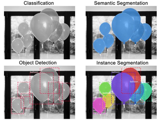
several computer-vision tasks that are similar and can confuse beginners. Example images [1]
containing several balloons are shown in Figure 1 to illustrate the following terminologies: image
classification, semantic segmentation, object detection, and instance segmentation.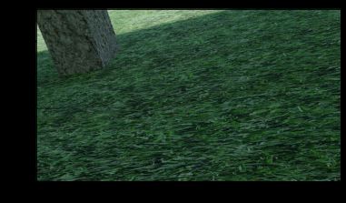
Figure 1. Illustration of computer vision tasks.

    Classification: There is balloon in this image.
    Semantic Segmentation: These are all the balloon pixels.
    Object Detection: There are 7 balloons in this image at these locations.
    Instance Segmentation: There are 7 balloons at these locations, and these are the pixels that
    belong to each one.

Deep learning methods including deep convolutional neural networks have demonstrated
tremendous success for these computer vision tasks in the past half decade. This tutorial walks the
user in the development of a simple deep convolutional neural network architecture for semantic
segmentation. For the network architecture, the authors of this tutorial followed a tutorial for
semantic segmentation available at [2].

Preparation
This tutorial has been tested in the following environment:

    Python version: 3.8.5
    tensorflow version: 2.5.0
    numpy version: 1.19.2
    cv2 version: 4.5.1
    matplotlib version: 3.3.2

The versions of these packages can be obtained by the following commands:
In [12]: import platform
print("Python version:", platform.python_version())
import sys
import os
import tensorflow as tf
print("tensorflow version:",tf.__version__)
import numpy as np
print("numpy version:",np.__version__)
import cv2
print("cv2 version:",cv2.__version__)
import matplotlib
from matplotlib import pyplot as plt
import matplotlib.image as mpimg
print("matplotlib version:",matplotlib.__version__)
import pandas as pd
print("pandas version:",pd.__version__)
from skimage.transform import resize
Python version: 3.8.8
tensorflow version: 2.5.0
numpy version: 1.19.5
cv2 version: 4.0.1
matplotlib version: 3.3.4
pandas version: 1.2.4
Loading the dataset
Let's first have a look at the dataset. The provided dataset is organized by four folders and four csv
files that stores the correspondences of image file names and the associated ground truth file
names (the readers should refer to the readme file for the details). Let's first read the csv file for
the training dataset and plot an image and the associamted label map.In [13]: path_ds = os.path.join('..','data_proj1','Tokaido_dataset_share') #put a path to
ftrain = pd.read_csv(os.path.join(path_ds,'files_train.csv'),header=None,index_co
print(ftrain.iloc[0])
image = mpimg.imread(os.path.join(path_ds,ftrain.iloc[0][0]))
print(image.shape)
print(type(image))
plt.imshow(image)
0 .\img_syn_raw\train\image_case0_frame0_Scene.png
1 .\synthetic\train\labcmp\image_case0_frame0.bmp
2 .\synthetic\train\labdmg\image_case0_frame0.bmp
3 .\synthetic\train\depth\image_case0_frame0.png
4 43.37547
5 True
6 True
Name: 0, dtype: object
(1080, 1920, 3)
Out[13]:In [14]: component_label = mpimg.imread(os.path.join(path_ds,ftrain.iloc[0][1]))
print(component_label.shape)
print(type(component_label))
plt.imshow(component_label)
print(np.min(component_label))
print(np.max(component_label))
(360, 640)
1
4
Since the primary purpose of this tutorial is the demonstration of a semantic segmentation method,
let's simplify the dataset here: we use the first 100 images from files_train.csv as the training data,
the next 10 images as the validation data, and the next 50 images as test data. The code below
read the training/validation/test set from the provided Tokaido dataset.
Tip: the way shown here is not optimal in terms of performance. The readers can take a look at [3]
for more detail.
There are 6 different types of components, represented by 1-6 Let's seperate it into 6 masks, one
for each component typeIn [22]: def rgb2gray(rgb):
r, g, b = rgb[:,:,0], rgb[:,:,1], rgb[:,:,2]
gray = 0.2989 * r + 0.5870 * g + 0.1140 * b
return gray
def create_dataset(ftrain,idx_row,path_ds):
N = len(idx_row)
train_x = []
train_y = []
for i in range(N):
idx = idx_row[i]
imageName = os.path.join(path_ds,ftrain.iloc[idx][0])
labName = os.path.join(path_ds,ftrain.iloc[idx][1])
input_array = rgb2gray(mpimg.imread(imageName))
input_array = resize(input_array, (input_array.shape[0] // 3, input_array
anti_aliasing=True)#downsample image so that its size is t
train_x.append(input_array)
mask = mpimg.imread(labName)
target_array = np.zeros((mask.shape[0],mask.shape[1],7))
target_array[:,:,0]=np.where(mask == 1, 1, 0)
target_array[:,:,1]=np.where(mask == 2, 1, 0)
target_array[:,:,2]=np.where(mask == 3, 1, 0)
target_array[:,:,3]=np.where(mask == 4, 1, 0)
target_array[:,:,4]=np.where(mask == 5, 1, 0)
target_array[:,:,5]=np.where(mask == 6, 1, 0)
target_array[:,:,5]=np.where(mask == 7, 1, 0)
train_y.append(target_array)
train_x = np.stack(train_x)
train_x = np.expand_dims(train_x, axis=3)
train_y = np.stack(train_y)
print(train_x.shape)
print(train_y.shape)
return train_x,train_y
In [23]: #create training dataset and the corresponding label
col_valid = ftrain[5]
idx_valid = [i for i in range(len(col_valid)) if col_valid[i]]
train_x,train_y = create_dataset(ftrain,idx_valid[:100],path_ds)
validation_x,validation_y = create_dataset(ftrain,idx_valid[100:110],path_ds)
test_x,test_y = create_dataset(ftrain,idx_valid[110:160],path_ds)
(100, 360, 640, 1)
(100, 360, 640, 7)
(10, 360, 640, 1)
(10, 360, 640, 7)
(50, 360, 640, 1)
(50, 360, 640, 7)In [25]: #Have a look at the image and the 7 masks
i = np.random.randint(len(train_x))
print(i)
fig, axes = plt.subplots(1, 8, figsize=(16, 112))
axes[0].imshow(train_x[i])
axes[1].imshow(train_y[i][:,:,0])
axes[2].imshow(train_y[i][:,:,1])
axes[3].imshow(train_y[i][:,:,2])
axes[4].imshow(train_y[i][:,:,3])
axes[5].imshow(train_y[i][:,:,4])
axes[6].imshow(train_y[i][:,:,5])
axes[7].imshow(train_y[i][:,:,6])
65
Out[25]:
In [27]: #Have a look at the image and the 7 masks
i = np.random.randint(len(validation_x))
print(i)
fig, axes = plt.subplots(1, 8, figsize=(16, 112))
axes[0].imshow(validation_x[i])
axes[1].imshow(validation_y[i][:,:,0])
axes[2].imshow(validation_y[i][:,:,1])
axes[3].imshow(validation_y[i][:,:,2])
axes[4].imshow(validation_y[i][:,:,3])
axes[5].imshow(validation_y[i][:,:,4])
axes[6].imshow(validation_y[i][:,:,5])
axes[7].imshow(validation_y[i][:,:,6])
3
Out[27]:
Applying a semantic segmentation algorithm (VERY
simple fully convolutional network)
Now let's train a simple network that performs the task of semantic segmentation. The fully
convolutional network [4], following the discussion in the semantic segmentation tutorial [3]. Fully
convolutional networks "take input of arbitrary size and produce correspondingly-sized output"
(Quoted from the abstract of [4]). The implementation discussed in [3] and herein is a very simple
version of the FCN in the sense that the resolution is constant from the input layer to the output
layer, without any max/average-pooling layers or skip connections. The readers of this tutorial are
encouraged to upgrade the network architectures with more advanced ones of their choice.In [34]: import tensorflow as tf
from tensorflow.keras import datasets, layers, models
tf.keras.backend.clear_session()
model = models.Sequential()
model.add(layers.Conv2D(filters=16, kernel_size=(3, 3), activation='relu', input_
model.add(layers.Conv2D(filters=32, kernel_size=(3, 3), activation='relu', paddin
model.add(layers.Conv2D(filters=32, kernel_size=(3, 3), activation='relu', paddin
model.add(layers.Conv2D(filters=32, kernel_size=(3, 3), activation='relu', paddin
model.add(layers.Conv2D(filters=32, kernel_size=(3, 3), activation='relu', paddin
model.add(layers.Conv2D(filters=32, kernel_size=(3, 3), activation='relu', paddin
model.add(layers.Conv2D(filters=32, kernel_size=(3, 3), activation='relu', paddin
model.add(layers.Conv2D(filters=32, kernel_size=(3, 3), activation='relu', paddin
model.add(layers.Conv2D(filters=32, kernel_size=(3, 3), activation='relu', paddin
model.add(layers.Conv2D(filters=16, kernel_size=(3, 3), activation='relu', paddin
model.add(layers.Conv2D(filters=train_y.shape[-1], kernel_size=(3, 3), activation
In [35]: model.summary()
Model: "sequential"
_________________________________________________________________
Layer (type) Output Shape Param #
=================================================================
conv2d (Conv2D) (None, 360, 640, 16) 160
_________________________________________________________________
conv2d_1 (Conv2D) (None, 360, 640, 32) 4640
_________________________________________________________________
conv2d_2 (Conv2D) (None, 360, 640, 32) 9248
_________________________________________________________________
conv2d_3 (Conv2D) (None, 360, 640, 32) 9248
_________________________________________________________________
conv2d_4 (Conv2D) (None, 360, 640, 32) 9248
_________________________________________________________________
conv2d_5 (Conv2D) (None, 360, 640, 32) 9248
_________________________________________________________________
conv2d_6 (Conv2D) (None, 360, 640, 32) 9248
_________________________________________________________________
conv2d_7 (Conv2D) (None, 360, 640, 32) 9248
_________________________________________________________________
conv2d_8 (Conv2D) (None, 360, 640, 32) 9248
_________________________________________________________________
conv2d_9 (Conv2D) (None, 360, 640, 16) 4624
_________________________________________________________________
conv2d_10 (Conv2D) (None, 360, 640, 7) 1015
=================================================================
Total params: 75,175
Trainable params: 75,175
Non-trainable params: 0
_________________________________________________________________In [36]: model.compile(optimizer='adam',
loss=tf.keras.losses.CategoricalCrossentropy(),
metrics=[tf.keras.metrics.BinaryAccuracy(),
tf.keras.metrics.Recall(),
tf.keras.metrics.Precision(),
tf.keras.metrics.MeanIoU(train_y.shape[-1])])
Now, let's train the model for 5 epochs.
In [ ]: history = model.fit(train_x, train_y, batch_size=4, epochs=5,
validation_data=(validation_x, validation_y))
In [50]: loss = history.history['loss']
val_loss = history.history['val_loss']
plt.figure()
plt.plot(history.epoch, loss, 'r', label='Training loss')
plt.plot(history.epoch, val_loss, 'bo', label='Validation loss')
plt.title('Training and Validation Loss')
plt.xlabel('Epoch')
plt.ylabel('Loss Value')
plt.legend()
plt.show()
Finally, let's perform basic validation:In [51]: # Evaluate the model on the test data using `evaluate`
print("Evaluate on test data")
results = model.evaluate(test_x, test_y, batch_size=1)
print("test results:", results)
Evaluate on test data
50/50 [==============================] - 12s 232ms/step - loss: 1.4408 - binary
_accuracy: 0.6522 - recall: 0.7793 - precision: 0.2604 - mean_io_u: 0.4286
test results: [1.4408271312713623, 0.6522330641746521, 0.7793354988098145, 0.26
03803277015686, 0.42857232689857483]
References
[1] Load images | TensorFlow Core. https://www.tensorflow.org/tutorials/load_data/images
(https://www.tensorflow.org/tutorials/load_data/images)
[2] https://awaywithideas.com/a-simple-example-of-semantic-segmentation-with-tensorflow-keras/
(https://awaywithideas.com/a-simple-example-of-semantic-segmentation-with-tensorflow-keras/)
[3] Load images | TensorFlow Core. https://www.tensorflow.org/tutorials/load_data/images
(https://www.tensorflow.org/tutorials/load_data/images)
[4] Long, J., Shelhamer, E., & Darrell, T. (2015). Fully Convolutional Networks for Semantic
Segmentation. IEEE Transactions on Pattern Analysis and Machine Intelligence, 39(4), 640–651.
https://doi.org/10.1109/TPAMI.2016.2572683 (https://doi.org/10.1109/TPAMI.2016.2572683)
In [ ]: You can also read