Introduction to Artificial Intelligence

CS 188                         Introduction to Artificial Intelligence
Spring 2023                                                                                      Note 10
These lecture notes are heavily based on notes originally written by Nikhil Sharma.
Last updated: January 15, 2023

Expectimax
We’ve now seen how minimax works and how running full minimax allows us to respond optimally against
an optimal opponent. However, minimax has some natural constraints on the situations to which it can re-
spond. Because minimax believes it is responding to an optimal opponent, it’s often overly pessimistic in
situations where optimal responses to an agent’s actions are not guaranteed. Such situations include scenar-
ios with inherent randomness such as card or dice games or unpredictable opponents that move randomly
or suboptimally. We’ll talk about scenarios with inherent randomness much more in detail when we discuss
Markov decision processes in the second half of the course.
This randomness can be represented through a generalization of minimax known as expectimax. Expecti-
max introduces chance nodes into the game tree, which instead of considering the worst case scenario as
minimizer nodes do, considers the average case. More specifically, while minimizers simply compute the
minimum utility over their children, chance nodes compute the expected utility or expected value. Our rule
for determining values of nodes with expectimax is as follows:

       ∀ agent-controlled states, V (s) =         max            V (s′ )
                                             s′ ∈successors(s)

                 ∀ chance states, V (s) =          ∑             p(s′ |s)V (s′ )
                                             s′ ∈successors(s)
                ∀ terminal states, V (s) =      known

In the above formulation, p(s′ |s) refers to either the probability that a given nondeterministic action results
in moving from state s to s′ , or the probability that an opponent chooses an action that results in moving
from state s to s′ , depending on the specifics of the game and the game tree under consideration. From this
definition, we can see that minimax is simply a special case of expectimax. Minimizer nodes are simply
chance nodes that assign a probability of 1 to their lowest-value child and probability 0 to all other children.
In general, probabilities are selected to properly reflect the game state we’re trying to model, but we’ll cover
how this process works in more detail in future notes. For now, it’s fair to assume that these probabilities
are simply inherent game properties.
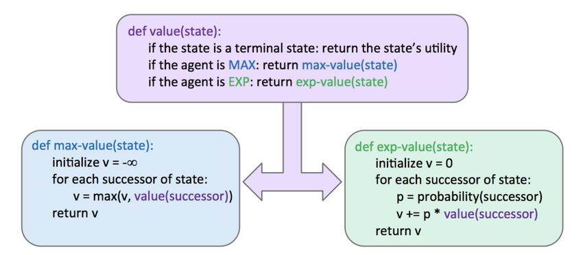
The pseudocode for expectimax is quite similar to minimax, with only a few small tweaks to account for
expected utility instead of minimum utility, since we’re replacing minimizing nodes with chance nodes:

CS 188, Spring 2023, Note 10                                                                                  1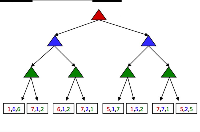

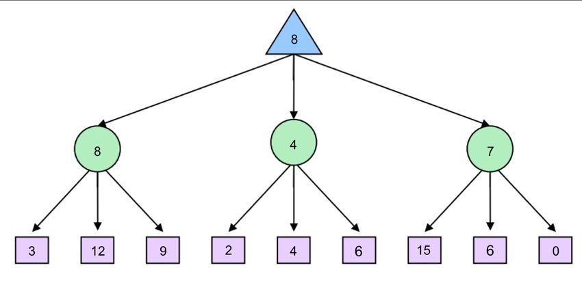
Before we continue, let’s quickly step through a simple example. Consider the following expectimax tree,
where chance nodes are represented by circular nodes instead of the upward/downward facing triangles for
maximizers/minimizers.

Assume for simplicity that all children of each chance node have a probability of occurrence of 13 . Hence,
from our expectimax rule for value determination, we see that from left to right the 3 chance nodes take on
values of 13 · 3 + 13 · 12 + 13 · 9 = 8 , 13 · 2 + 13 · 4 + 13 · 6 = 4 , and 31 · 15 + 13 · 6 + 13 · 0 = 7 . The maximizer
selects the maximimum of these three values, 8 , yielding a filled-out game tree as follows:

CS 188, Spring 2023, Note 10                                                                                            2

As a final note on expectimax, it’s important to realize that, in general, it’s necessary to look at all the
children of chance nodes – we can’t prune in the same way that we could for minimax. Unlike when
computing minimums or maximums in minimax, a single value can skew the expected value computed by
expectimax arbitrarily high or low. However, pruning can be possible when we have known, finite bounds
on possible node values.

Mixed Layer Types
Though minimax and expectimax call for alternating maximizer/minimizer nodes and maximizer/chance
nodes respectively, many games still don’t follow the exact pattern of alternation that these two algorithms
mandate. Even in Pacman, after Pacman moves, there are usually multiple ghosts that take turns making
moves, not a single ghost. We can account for this by very fluidly adding layers into our game trees as
necessary. In the Pacman example for a game with four ghosts, this can be done by having a maximizer
layer followed by 4 consecutive ghost/minimizer layers before the second Pacman/maximizer layer. In fact,
doing so inherently gives rise to cooperation across all minimizers, as they alternatively take turns further
minimizing the utility attainable by the maximizer(s). It’s even possible to combine chance node layers with
both minimizers and maximizers. If we have a game of Pacman with two ghosts, where one ghost behaves
randomly and the other behaves optimally, we could simulate this with alternating groups of maximizer-
chance-minimizer nodes.

As is evident, there’s quite a bit of room for robust variation in node layering, allowing development of
game trees and adversarial search algorithms that are modified expectimax/minimax hybrids for any zero-
sum game.

Monte Carlo Tree Search
For applications with a large branching factor, like playing Go, minimax can no longer be used. For such
applications we use the Monte Carlo Tree Search (MCTS) algorithm. MCTS is based on two ideas:

    • Evaluation by rollouts: From state s play many times using a policy (e.g. random) and count wins/losses.

    • Selective search: explore parts of the tree, without constraints on the horizon, that will improve deci-
      sion at the root.

In the Go example, from a given state, we play until termination according to a policy multiple times. We
record the fraction of wins, which correlates well with the value of the state.

CS 188, Spring 2023, Note 10                                                                                3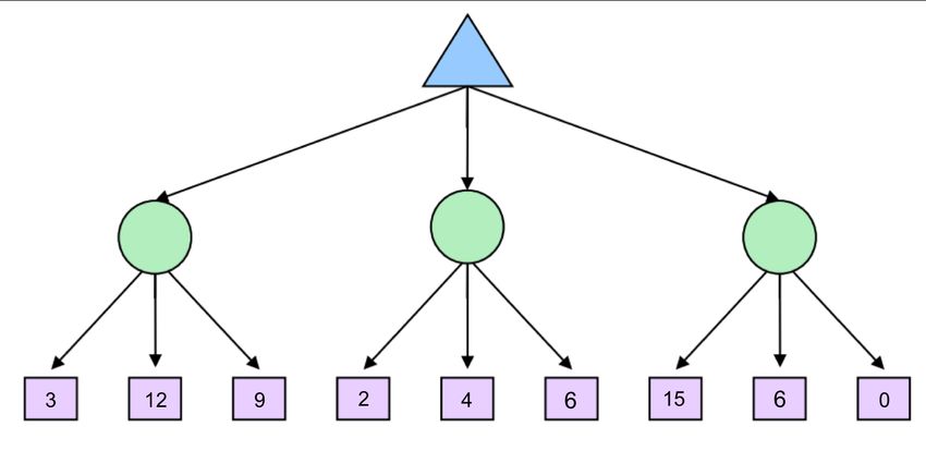

Consider the following example:

From the current state we have three different available actions (left, middle and right). We take each action
100 times and we record the percentage of wins for each one. After the simulations, we are fairly confident
that the right action is the best one. In this scenario, we allocated the same amount of simulations to each
alternative action. However, it might become clear after a few simulations that a certain action does not
return many wins and thus we might choose to allocate this computational effort in doing more simulations
for the other actions. This case can be seen in the following figure, where we decided to allocate the
remaining 90 simulations for the middle action to the left and right actions.

An interesting case arises when some actions yield similar percentages of wins but one of them has used
much fewer simulations to estimate that percentage, as shown in the next figure. In this case the estimate of
the action that used fewer simulations will have higher variance and hence we might want to allocate a few
more simulations to that action to be more confident about the true percentage of wins.

The UCB algorithm captures this trade-off between “promising" and “uncertain’ actions by using the fol-
lowing criterion at each node n:

CS 188, Spring 2023, Note 10                                                                                4

s
                                         U(n)                 log N(PARENT (n))
                               UCB1(n) =      +C ×
                                         N(n)                        N(n)

where N(n) denotes the total number of rollouts from node n and U(n) the total number of wins for
Player(Parent(n)). The first term captures how promising the node is, while the second captures how
uncertain we are about that node’s utility. The user-specified parameter C balances the weight we put in
the two terms (“exploration" and “exploitation") and depends on the application and perhaps the stage of
the task (in later stages when we have accumulated many trials, we would probably explore less and exploit
more).
The MCTS UCT algorithm uses the UCB criterion in tree search problems. More specifically, it repeats the
following three steps multiple times:

   1. The UCB criterion is used to move down the layers of a tree from the root node until an unexpanded
      leaf node is reached.

   2. A new child is added to that leaf, and we run a rollout from that child to determine the number of wins
      from that node.

   3. We update the numbers of wins from the child back up to the root node.

Once the above three steps are sufficiently repeated, we choose the action that leads to the child with the
highest N. Note that because UCT inherently explores more promising children a higher number of times,
as N → ∞, UCT approaches the behavior of a minimax agent.

General Games
Not all games are zero-sum. Indeed, different agents may have have distinct tasks in a game that don’t
directly involve strictly competing with one another. Such games can be set up with trees characterized by
multi-agent utilities. Such utilities, rather than being a single value that alternating agents try to minimize or
maximize, are represented as tuples with different values within the tuple corresponding to unique utilities
for different agents. Each agent then attempts to maximize their own utility at each node they control,
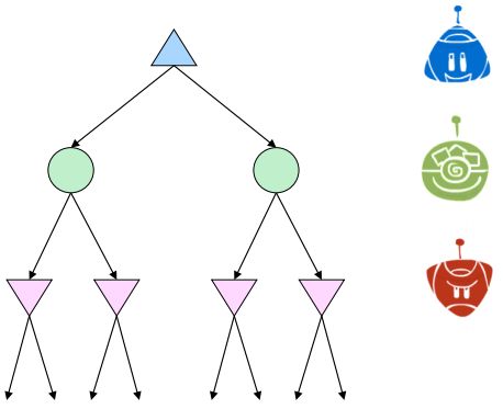
ignoring the utilities of other agents. Consider the following tree:

CS 188, Spring 2023, Note 10                                                                                    5

The red, green, and blue nodes correspond to three separate agents, who maximize the red, green, and blue
utilities respectively out of the possible options in their respective layers. Working through this example
ultimately yields the utility tuple (5, 2, 5) at the top of the tree. General games with multi-agent utilities are
a prime example of the rise of behavior through computation, as such setups invoke cooperation since the
utility selected at the root of the tree tends to yield a reasonable utility for all participating agents.

Summary
In this note, we shifted gears from considering standard search problems where we simply attempt to find a
path from our starting point to some goal, to considering adversarial search problems where we may have
opponents that attempt to hinder us from reaching our goal. Two primary algorithms were considered:

    • Minimax - Used when our opponent(s) behaves optimally, and can be optimized using α-β pruning.
      Minimax provides more conservative actions than expectimax, and so tends to yield favorable results
      when the opponent is unknown as well.

    • Expectimax - Used when we facing a suboptimal opponent(s), using a probability distribution over
      the moves we believe they will make to compute the expectated value of states.

In most cases, it’s too computationally expensive to run the above algorithms all the way to the level of
terminal nodes in the game tree under consideration, and so we introduced the notion of evaluation func-
tions for early termination. For problems with large branching factors we described the MCTS and UCT
algorithms. Such algorithms are easily parallelizable, allowing for a large number of rollouts to take place
using modern hardware.
Finally, we considered the problem of general games, where the rules are not necessarily zero-sum.

CS 188, Spring 2023, Note 10                                                                                    6