APPLICATION OF EVA FOR CLIMATE CHANGE ADAPTATION - ALEXIS HANNART OURANOS AND MCGILL UNIVERSITY
←
→
Page content transcription
If your browser does not render page correctly, please read the page content below
Application of EVA
for climate change adaptation

         Alexis Hannart
   Ouranos and McGill University

          30 October 2019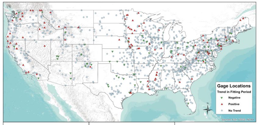
Outline

  ⚫   Context and motivation

  ⚫   Approach in a stationary climate

  ⚫   Bringing climate change into the picture

  ⚫   Conclusion
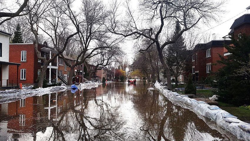
Québec
Québec
Montreal, April 2017
Québec, April 2019
Streamflow, Rouge River

                 Streamflow time series

                 Streamflow histogram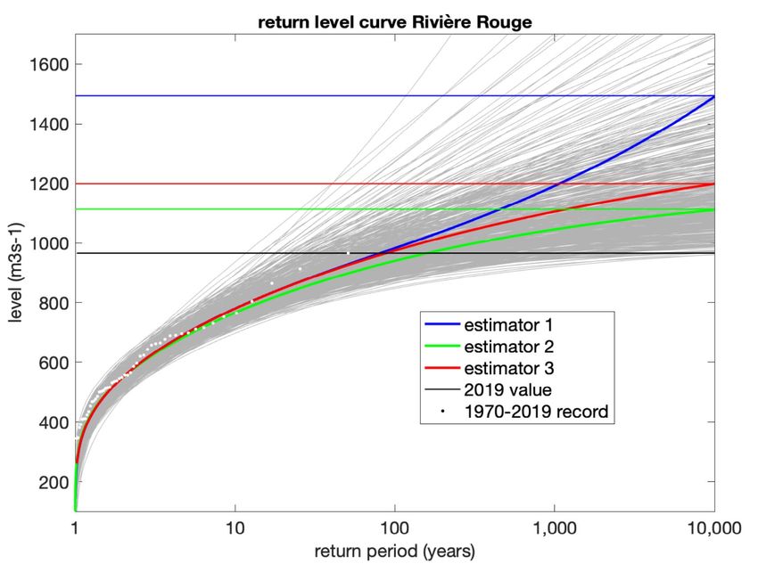
Streamflow, Rouge River

                 Streamflow time series

                 Streamflow histogram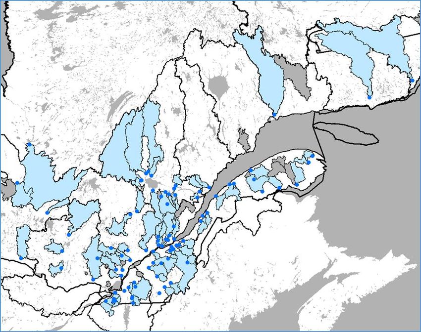
Attributing extreme events to climate change

⚫   Attribution requires to computes the probabilities p0 and p1 that a given
    observed value u (e.g. 2019 record streamflow) is exceeded.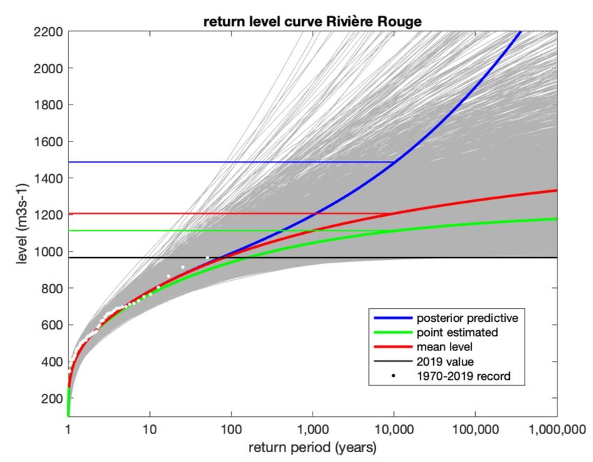
Attributing extreme events to climate change

⚫   Attribution requires to computes the probabilities p0 and p1 that a given
    observed value u (e.g. 2019 record streamflow) is exceeded.

⚫   From there, several causal metrics can be derived:
Question asked for attribution
What is the value of the probability to exceed a given threshold?
⚫ The threshold is high and may never have been reached in
observations (e.g. counterfactual).Designing maps of flood risk
Return level Digital Elevation Map Map of
curve + Flood model flood riskQuestion asked for flood risk mapping
What are the values of the 20, 50 and 100 years flow ?
⚫ The regulator will enforce only one map in the law. The answer is
requested to be a single value.Question asked for flood risk mapping
What are the values of the 95%, 98% and 99% quantile ?
⚫ The regulator will enforce only one map in the law. The answer is
requested to be a single value.Hydropower generation
Hydropower generation
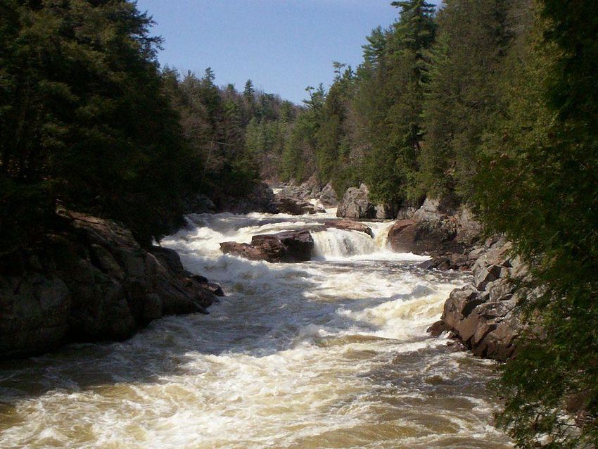
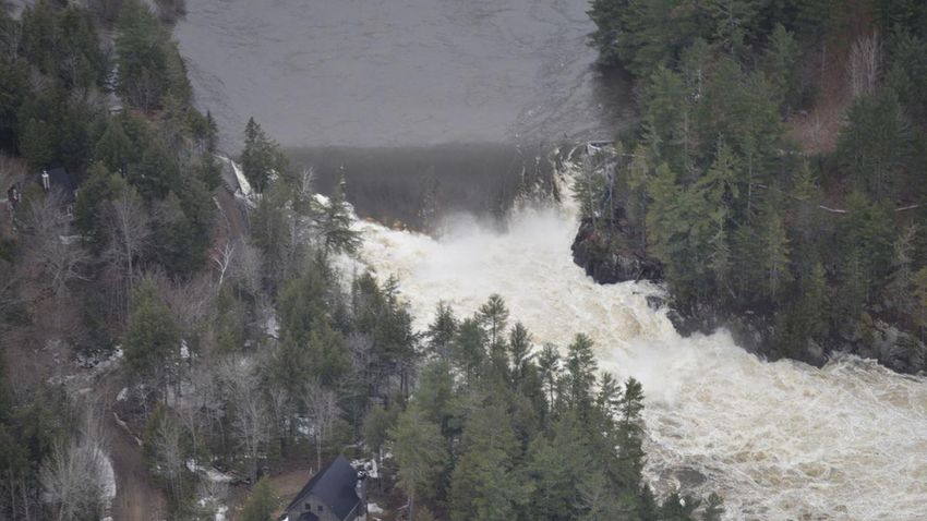
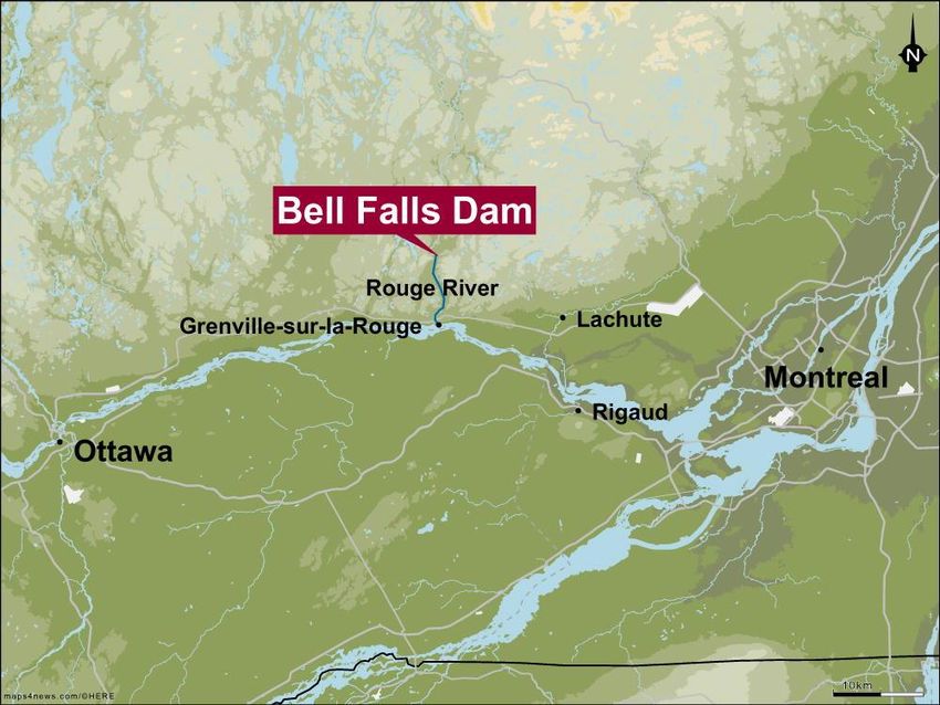
Bell Falls, Rouge River
Streamflow, Rouge River

                 Streamflow time series

                 Streamflow histogram
Spillways
A spillway is a
structure used to
release the surplus
of flow from a dam
into a downstream
area.
Streamflow histogramBell Falls, April 2019
Bell Falls, April 2019
Decision making under uncertainty
Decision making under uncertainty

                                         consequences
                                         of dam failure
                                         very high

                        consequences
                        of dam failure
                        moderate

       consequences
       of dam failure
       low
Dam Safety Act, Chapter S-3.1.01
Question asked by hydropower companies and
        regulating bodies

          What is the value of the 10,000 years flow ?

⚫   Civil engineers designing the spillway will build one spillway. The
    answer is requested to be a single value.
Question asked by hydropower companies and
regulating bodies
What is the value of the 99,99% quantile ?
⚫ Civil engineers designing the spillway will build one spillway. The
answer is requested to be a single value.Problem Estimate a high quantile for a given low probability Estimate a low probability for a given high threshold
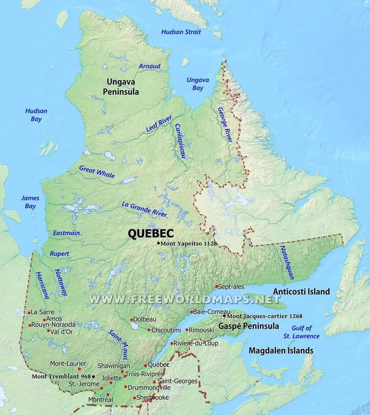
Hydrological map of the area

                 Gauge station database = 88 stations
Outline ⚫ Context and motivation ⚫ Approach in a stationary climate ⚫ Bringing climate change into the picture ⚫ Conclusion
Streamflow, Rouge River

                 Streamflow time series

                 Streamflow histogram
Data: annual maxima
Model: univariate Generalized Extreme Value distribution
Inference: maximum likelihood
Comparison with the GPD model
Inference: maximum likelihood

         Can we come up with a better estimator ?
Bayesian estimation: a brief overview
Bayesian estimation: a brief overview

                                MCMC simulations
Model: univariate Generalized Extreme Value distribution
Northrop and Attalides 2015MCMC simulation of the posterior distribution
MCMC simulation of the posterior return level curve
MCMC simulation of the posterior PDF of the probability of
exceedance
A probability on a probability ?

                             P(P(X>u)u) = 0.0132, or 75 years return period
A probability on a probability ?
This probabilty is called the posterior predictive
A probability density on a probability can (arguably should)
always be boiled down to a single number.
In this case, P(X>u) = 0.0132, or 75 years return periodThe posterior predictive: a possible estimator of the return level curve
Bayesian estimation: a brief overview
MCMC simulationsBayesian estimation: a brief overview
Bayesian estimation: a brief overview
Bayesian estimation: a brief overview
Model: univariate Generalized Extreme Value distribution
Attempt 1: conventional cost function and estimator
Attempt 2: conventional cost function and estimator
Attempt 3: new cost function and estimator
Attempt 4: new cost function and estimator
Attempt 5: new cost function and estimator
Attempt 6: new cost function and estimator
The posterior predictive: a possible estimator of the return
level curve
Illustration on Rouge River

                                             Estimator #1

                              Estimator #2
Properties and performance of estimators
Simulation testbed results for p = 10-2 and xi < 0
Simulation testbed results for p = 10-4 and xi < 0
Simulation testbed results for p = 10-2 and xi > 0
Simulation testbed results for p = 10-4 and xi > 0
Preliminary conclusion

⚫   Even for a single parametric model, several different point estimators of high
    quantiles and low probabilities can be proposed.

⚫   Within a Bayesian approach, such estimators can be obtained by choosing
    alternative cost functions that are ad-hoc to the problem.

⚫   The conventional estimator of a high quantile (inverse CDF evaluated at p with
    MLE of theta) is not necessarily the best solution. Neither is the intuitive solution of
    the « posterior predictive ».

⚫   Instead, the « MAP quantile » estimator appears to consistently perform best,
    based on simulation results.

⚫   More simulation and theoretical grounding for these estimators is needed.

⚫   Significant implications for high quantiles.
Outline ⚫ Context and motivation ⚫ Approach in a stationary climate ⚫ Bringing climate change into the picture ⚫ Conclusion
Spring floods 2017 and 2019

                 Avril 2017                          Avril 2019

Read in the media:

⚫   « These events are more and more frequent, and they will become even more
    frequent in the future. »

                                                                  Source: GéoMSP, Québec
Spring floods 2017 and 2019
Avril 2017 Avril 2019
Return period: 50 years Return period: 50 years
Two in three years:
Return period 850 years
under independance assumptionQuestions
Avril 2017 Avril 2019
⚫ What is the influence of CC on flood risk in Québec ?
⚫ How can it be taken into account in the new flood risk maps ?Overall workplan
thématique axe de recherche projet expertise % 2019 2020 2021 2022 2023
documentation des crues
modélisation hydraulique
Incidence du analyse, détection et hydro, climat,
Projet 1.1 17%
Axe 1
changement attribution stat, obs
climatique sur les production des simulations
Projet 1.2 hydro, climat 3%
crues contrefactuelles
modèles, simulations et
Projet 2.1 climat, stat, obs 12%
observations climatiques
modèles, simulations et hydro, climat,
Projet 2.2 12%
observations hydrologiques stat, obs
Modélisation
Axe 2
évolution nouvelles simulations
hydroclimatique et Projet 2.3 hydro 6%
du climat hydrologiques
incertitudes
Projet 2.4 analyse fréquentielle stat, hydro 15%
intégration et transition vers
Projet 2.5 hydro, crues, obs 15%
l’hydraulique fluviale
Projet 3.1 veille et analyses ad-hoc com, ad-hoc 10%
Axe 3
Questions pointues et
divulgation communication de la qualité com, hydro,
Projet 3.2 10%
des résultats climat, stat, obs
⚫ 3 years,
⚫ ~7m CAD,
⚫ ~30 people.Outline ⚫ Context and motivation ⚫ Approach in a stationary climate ⚫ Bringing climate change into the picture: detection ⚫ Conclusion
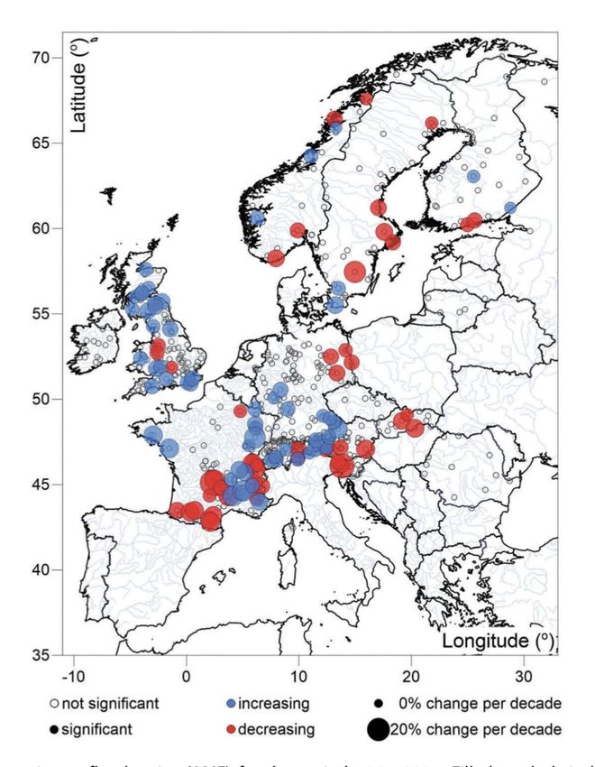
Detection: is there a change ?

   frequency                                    duration

                   Dartmouth Flood Observatory database

                                                     Najibi et al. 2018
Detection: is there a change ?
USGS database
Luke et al. 2017Detection: is there a change ?
USGS database
Luke et al. 2017Detection: is there a change ?
GRDC database
Mangini et al. 2018Detection: is there a change ?
Gauge station database
Burn et al. 2010
Burn and Withfield 2018Detection: is there a change ?
Gauge station database
Hannart et al. EVA 2019Outline ⚫ Context and motivation ⚫ Approach in a stationary climate ⚫ Bringing climate change into the picture: attribution ⚫ Conclusion
Hypothetical drivers

            Snowpack

            Snowmelt
Climate
Change
                          Streamflow
             Rainfall
                                         Flooding
                                 River
             ETP

             River

            Catchment

                                                    after Kreibich et al. 2019
Hypothetical drivers
Snowpack
Snowmelt
Climate
Change
Streamflow Frequency
Rainfall
Flooding
River Magnitude/Duration
ETP
River
Catchment
after Kreibich et al. 2019Hypothetical drivers
Snowpack
Snowmelt
Climate
Change
Streamflow Frequency
Rainfall
Flooding
River Magnitude/Duration
ETP
Damages
Exposure
River
Vulnerability
Catchment
after Kreibich et al. 2019Hypothetical drivers
Snowpack Shift from nival regime to mixed regime
– Shift from mixed regime to pluvial regime
Snowmelt
Climate –
Change
Streamflow Frequency
Rainfall
+ +/– Flooding
River +/– Magnitude/Duration
ETP
River
Catchment
after Kreibich et al. 2019Two main antagonic effects
Couvert neigeux (MTL) Précipitation avril (MTL)
mm
mm
1940 1980 2020 1940 1980 2020
Source: ECCCProjected changes (ISI-MIP)
increase
constant
decrease
Source: Asadieh and Krakauer 2017Projected changes (CQ2)
Crue 20 ans, RCP8.5, 2050
increase
constant
decrease
Source: Atlas 2018, DEH/OuranosNumerical experiments
Précipitation avril (MTL) Couvert neigeux (MTL) Débit avril (MTL)
niveau observé en 2017 simulation climat présent simulation climat passé
Pluie: Couvert neigeux: Débit:
augmentation baisse pas de modification
de la fréquence de la fréquence de la fréquence.
~ facteur 2 ~ facteur 2
Source: Teufel et al. 2018Large uncertainty in hydroclimatic model response
Giuntoli et al. 2018Large uncertainty in hydroclimatic model response
Réponse moyenne Dispersion générée Dispersion générée
de tous les modèles par les modèles climat par les modèles hydro
%
Giuntoli et al. 2018Outline ⚫ Context and motivation ⚫ Approach in a stationary climate ⚫ Bringing climate change into the picture: mapping ⚫ Conclusion
Mapping: models and observations in cascade

⚫   Schéma conceptuel d’un modèle de calcul de cartographie du risque de crue.

Sampson et al. 2015           Dottori et al. 2016              Trigg et al. 2016
Computation: models and observations in cascade

Observations            Observations              Observations            Observations
émissions               climatiques               hydrologiques           crues

               Modèle(s)                 Modèle(s)                Modèle                        Produit
               Climatique                Hydrologique             Hydraulique                   fini

   Scénarios                Post-processing
                            Post-traitement        Post-processing
                                                   Post-traitement              Calcul
   émissions                climatique             hydrologique                 d’indicateurs
                                                                                & cartes

                      Solution retenue: schéma en cascade complet.
Computation: models and observations in cascade
incertitude cumulative intégration de
en cascade l’incertitude calcul
non stationnarité déterministe
5 10 15
101 102 103
Modèle(s) Modèle(s) Modèle Produit
Climatique Hydrologique Hydraulique finiRouge River sampling uncertainty
Climate change uncertainty effect on return levels
Climate change uncertainty effect on return levels
Agenda

 ⚫   Context and motivation

 ⚫   Model and inference

 ⚫   Results

 ⚫   Conclusion
Conclusion

⚫   Estimating high quantiles is difficult.

⚫   The GEV extrapolation has many well-known (and less well-known)
    problems, but still the ‘least worst’ option by default thus far.

⚫   Physics may come to the rescue of statistics.
    —   careful attribution of extremes to identify drivers,
    —   careful modelign of the dependence between drivers.

⚫   Building climate change into the picture complexifies what is already a
    difficult problem.

⚫   How to do this in practice is an active and interesting area of research.
Thank you
You can also read


