Three dimensional atmospheric entry simulation of a high altitude cometary dustball meteoroid
←
→
Page content transcription
If your browser does not render page correctly, please read the page content below
A&A 650, A101 (2021)
https://doi.org/10.1051/0004-6361/202140305 Astronomy
c ESO 2021 &
Astrophysics
Three dimensional atmospheric entry simulation of a high altitude
cometary dustball meteoroid
L. Hulfeld, S. Küchlin, and P. Jenny
Institute of Fluid Dynamics, Swiss Federal Institute of Technology (ETH) in Zurich, Sonneggstrasse 3, 8092 Zürich, Switzerland
e-mail: lorenz.hulfeld@gmail.com
Received 9 January 2021 / Accepted 7 April 2021
ABSTRACT
Aims. The break-up of a dustball meteoroid is investigated numerically based on fluid dynamics simulations of the meteoroid’s atmo-
spheric entry flow. Both thermal and mechanical break-up mechanisms are implemented, in order to investigate dustball meteoroid
disintegration.
Methods. A three dimensional model of a dustball meteoroid composed of thousands of small spherical grains was used in the atmo-
spheric entry flow simulation, performed with the direct simulation Monte Carlo (DSMC) method. The dynamics of each meteoroid
grain were calculated by means of the discrete element method (DEM), which models contact dynamics between grains. By coupling
DEM with DSMC, the dynamics of a dustball meteoroid were calculated during atmospheric entry. In addition, thermal computa-
tions were also carried out taking into account the incoming atmospheric heat flux, thermal radiation, and grain ablation. Thus, this
methodology is able to compute mechanical as well as thermal dustball meteoroid disintegration.
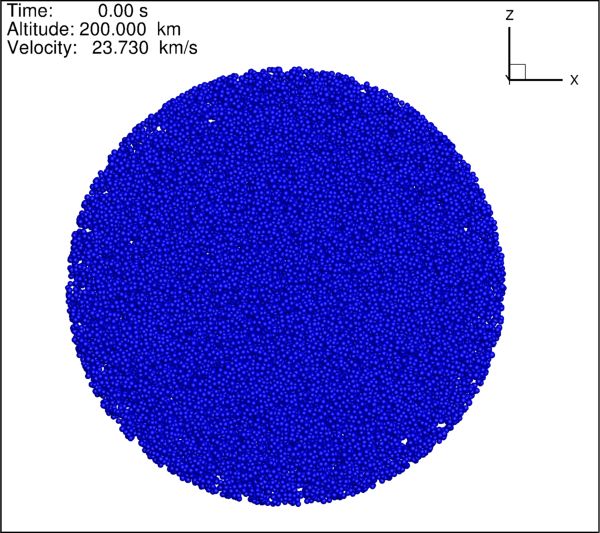
Results. To test this novel multi-physics simulation framework, a prototypical dustball meteoroid, namely a Draconid meteoroid, was
simulated. Using typical material properties from the literature, the Draconid meteoroid was compressed due to aerodynamic forces
to roughly half its size immediately after the start of the simulation at 200 km altitude. Later, aerodynamic-induced meteoroid rotation
occured until the meteoroid disintegrated mechanically at 120 km altitude. The fact that the meteoroid disintegrated mechanically is
directly related to the combination of material properties used in the simulation.
Key words. meteorites, meteors, meteoroids – methods: miscellaneous
1. Introduction erosion, that is to say grains detach from the meteoroid surface
after they receive a certain amount of thermal energy from the
Jacchia (1955) concluded from Super-Schmidt photographic atmospheric flow.
observations that fragmentation of small meteoroids during The dustball models by Campbell-Brown & Koschny and
atmospheric entry is a common phenomenon. In accordance with Borovička et al. were recently compared against each other
Whipple’s cometary model (Whipple 1951), he concluded on by fitting high resolution observations of several faint mete-
the basis of these observations that meteoroids must be porous ors (Campbell-Brown et al. 2013). The authors conclude that
dustballs. dustball models need to be improved significantly to fit the
Hawkes & Jones (1975) developed the first quantitative dust- observations. Thus, rather than using simple analytical mod-
ball model and assumed that dustball meteoroids consist of els, we decided to simulate the atmospheric entry flow about a
stony or metallic grains embedded in a matrix of non-radiating three dimensional dustball meteoroid. As dustball meteoroids are
volatile “glue”. They assumed that dustball meteoroids continu- mostly of cometary origin, the dustball model proposed in this
ously release grains during atmospheric entry as the glue melts. paper was derived from the structure and formation of comets.
They presumed that a dustball meteoroid has released all of its Comets formed early in the Solar System, about 4.6 G.y. ago,
grains before the onset of ablation. Their model was able to fit beyond the snow line and their composition has not evolved sig-
light curves of different meteor types (Hawkes & Jones 1975; nificantly since (Fernandez 2004; Mandt et al. 2015). Blum et al.
Fisher et al. 2000). (2014) found, based on the model by Skorov & Blum (2012),
More recently, Campbell-Brown & Koschny (2004) devel- that comets must have formed from porous dust and ice aggre-
oped a more qualitative dustball model. They adopted the gates by gravitational instabilities. Whenever a comet passes
assumption that dustball meteoroids are held together by a sort the inner Solar System, icy parts of the comet sublimate and
of glue and simulated heat conduction in the meteoroid and the the comet releases gas and dust. These dust aggregates (i.e.,
release of grains where the glue reached the melting temperature. dustballs) remain approximately in the comet’s orbit and every
In contrast to Hawkes & Jones’s model, grain ablation was simu- time when Earth crosses a comets’ orbit, theses dustball mete-
lated on the basis of each grain’s temperature using the Clausius- oroids ablate during atmospheric entry, producing meteor show-
Clapeyron equations, thus allowing for grain ablation before the ers (Greenberg 2000). Thus, by studying dustball meteoroids,
dustball meteoroid which is fully disintegrated. we can gain knowledge about their parent comets and because
The most recent dustball model was proposed by comets have not evolved significantly since their formation, they
Borovička et al. (2007). Their model does not presume a matrix provide a valuable record of the physical conditions in the early
of volatile glue. The grains are released based on thermal Solar System.
Article published by EDP Sciences A101, page 1 of 16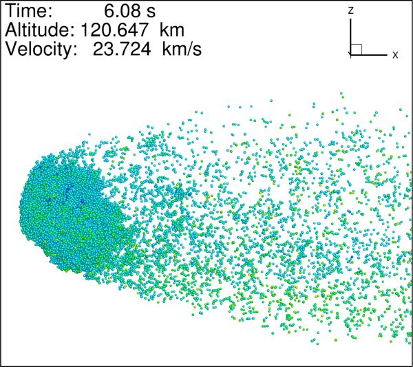
A&A 650, A101 (2021)

     In the early Solar System, the gas surrounding the Sun (solar         Stokan & Campbell-Brown (2015) used a particle-based
nebula) condensed into dust and ice particles, which led to           method to simulate the ablation and deceleration of small non-
the formation of the protoplanetary disk (PPD; Bouwman et al.         fragmenting meteoroids. On the basis of collisions between par-
2008). These dust and ice grains subsequently formed small            ticles, the light emission of meteors was simulated. They found
aggregates since they stuck together by adhesion after inelastic      good agreement between the width of simulated meteor wakes
collisions (Weidenschilling & Cuzzi 1993). Experiments con-           and observations. However, their simulated meteors showed less
cerning the formation of protoplanetary dust aggregates were          deceleration and shorter wakes than observed, which led to the
conducted in the last two decades by numerous researchers.            conclusion that meteoroid fragmentation plays an important role
Below, a few of these papers are summarized; a more complete          in the observed small meteoroids.
review can be found in Blum & Wurm (2008).                                 Although rarely used until present, particle-based methods
     Poppe et al. (2000a) performed collisions between micron-        have shown very promising results and DEM has been estab-
sized grains, corresponding to the first step of planetesimal and     lished in the field of astrophysical research. By combining both
cometesimal formation in the solar nebula. They experimen-            methods, a simulation based on the physics of the atmospheric
tally confirmed that due to Brownian motion collisions between        entry of a dustball meteoroid should be performed. The dynam-
micron-sized dust particles lead to sticking and subsequently to      ics of each meteoroid grain is simulated with DEM and the
the formation of small fractal dust aggregates. Blum & Wurm           atmospheric entry flow is computed by a highly flexible DSMC-
(2000) investigated collisions between fractal dust aggregates        Fokker-Planck algorithm (Küchlin & Jenny 2017). By coupling
in a micro gravity environment. They found that below a               DEM to the atmospheric entry flow computation, the dynamics
threshold velocity, the fractal dust aggregates stick together        of a dustball meteoroid during its flight through the atmosphere
after a collision, forming bigger, very porous non-fractal dust       can be investigated. Ablation of the meteoroid grains is calcu-
aggregates. Blum et al. (2006) produced dust aggregates in the        lated and compared to measurements of dustball meteoroids in
laboratory by random ballistic deposition. The resulting              order to validate the model.
centimeter-sized aggregates showed good agreement of porosity
and tensile strength with meteoroids of cometary origin.              2. Meteoroid model
     Based on numerous laboratory experiments done in the last
two decades, Güttler et al. (2010) and Zsom et al. (2010) showed      As mentioned in the introduction, there is strong evidence that
that dust aggregates up to a centimeter in size can form in the       comets consist of loosely bound dust and ice aggregates and
PPD due to collisional growth. Thus, there is strong evidence         thus that cometary meteoroids are dust aggregates. Blum et al.
that cometary meteoroids are aggregates of small dust grains. In      (2006) showed that such dust aggregates have porosities and
addition to laboratory experiments about the formation of dust        tensile strengths similar to cometary meteoroids. Therefore, the
aggregates in the PPD, computational studies were done as well.       assumption was made that dustball meteoroids are loosely bound
     Dominik & Tielens (1997) modeled normal adhesive forces          aggregates of their constituent grains and that they are held
and rolling, sliding, and torsional friction between two interact-    together by mechanical forces and not by some sort of nonra-
ing dust grains. On the basis of these contact laws, they devel-      diating glue.
oped a two dimensional discrete element method (DEM) code                 In the first step of planetesimal and cometesimal formation,
and applied it to the formation and collision of dust aggregates      fractal dust aggregates form in the PPD due to hit and stick
in the PPD. More recently, Wada et al. (2007, 2008) carried out       collisions of dust grains, which subsequently collide with each
similar two and three dimensional DEM computations of col-            other forming nonfractal, bigger, very porous dust aggregates
lisions between two dust aggregates. Ringl & Urbassek (2012)          (Poppe et al. 2000a; Blum & Wurm 2000). Therefore, the struc-
developed a simplified model of adhesion rolling, gliding, and        ture of a cometary dust ball meteoroid is modeled in this paper
torsional friction for grain-grain interactions. Their simplified     as a nonfractal porous agglomeration of grains. The meteoroid
code allows for faster simulations with more particles than the       should be characterized by a certain porosity and is assumed
codes by the authors introduced above. Their code was applied         to have a homogeneous structure throughout. Since the initial
in the PPD context (Gunkelmann et al. 2016, 2017). The use of         geometry of a meteoroid entering Earth’s atmosphere cannot be
DEM in astrophysical research has been established over the last      measured yet, the dustball meteoroid is assumed to have a nearly
two decades. Therefore, we decided to apply DEM to model a            perfect spherical shape. Because of simplicity and to speed up
dustball meteoroid.                                                   the simulations presented in this paper, all grains were modeled
     Due to the rarefied nature of the atmospheric entry flow about   as perfect spheres.
a dustball meteoroid, a particle-based simulation technique is
best suited. Although very promising, particle-based flow sim-
                                                                      2.1. Grain bonds
ulations have very rarely been used in meteor science. The fol-
lowing publications are known to us.                                  We assume that the constituent grains are only held together
     Boyd (2000) used the direct simulation Monte Carlo               by adhesive forces, although grains may also be held together
(DSMC) method to compute the flow filed around a 1 cm-sized           by electromagnetism (Dominik & Nübold 2002). The adhesive
Leonid meteoroid during atmospheric entry. He performed a sta-        force between two grains is modeled according to the DMT
tionary DSMC computation of the ablating meteoroid at an alti-        model (Derjaguin et al. 1975) as
tude of 95 km. The wake behind the ablating meteoroid in the
simulation was in quantitative agreement with measurements.           FAdh = 4πγrred ,                                              (1)
     Vinković (2007) used DSMC to simulate high altitude
Lenoids above 130 km. He used a model in which meteoroid              where γ denotes the surface energy and rred is the reduced radius
particles were ejected from the surface to simulate sputtering of     of the two grains, which is defined as
high altitude meteors. The results of his DSMC computations
show good agreement with measured shapes and sizes of high             1   1  1
                                                                          = + .                                                     (2)
altitude Leonids.                                                     rred ri r j

A101, page 2 of 16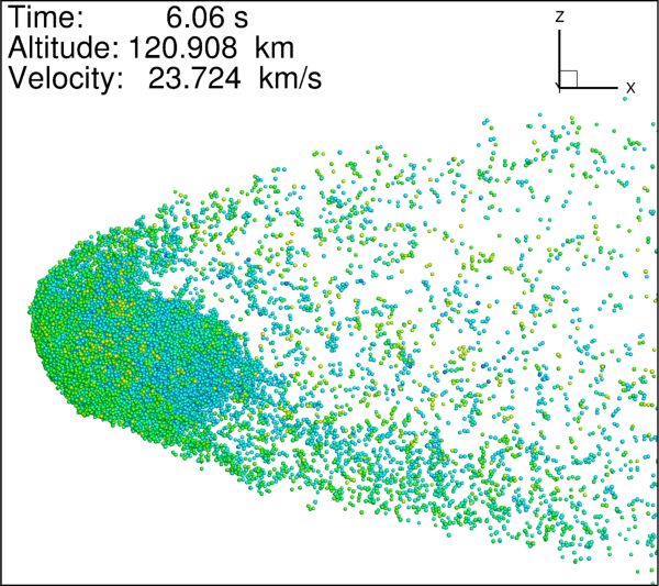
L. Hulfeld et al.: Atmospheric entry simulation of a dustball meteoroid
The repulsive force between two grains is modeled by the grain overlapped with another grain, its position was calculated
Hertzian theory (Hertz 1881) as such that it had equilibrium overlap with both grains. After a new
grain was attached to the meteoroid, the porosity of the mete-
2 E √ oroid was calculated by summing up the volume of all present
FHertz = rred δi3/2
j , (3)
3 1 − v2 grains and dividing it by the volume of their convex hull. If the
where E denotes the Young modulus and v is the Poisson ratio meteoroid’s porosity was too low, grains were removed until the
of the grains. The overlap σ of two grains is obtained as desired porosity was reached. If the meteoroid did not remain in
one piece after the removal of a grain, this grain must not have
been removed.
δi j = max ri + r j − |xi − x j |, 0 , (4)
where xi and x j denote the grains’ centroids. When two grains
stick together, elastic deformation leads to the formation of a 2.4. Heat transfer
circular area between the grains. The radius of the contact area The temperature of each meteoroid grain was calculated as
Ai j = πa2i j between two grains is given by Hertzian theory (Hertz
1881) as ∂T i
c p mi = qi,conv + qi,rad + qi,cond + qi,mass , (10)
∂t
ai j = δi j rred . (5)
p
where qi,conv , qi,rad , qi,cond , and qi,mass denote a grain’s convective,
The equilibrium overlap of two grains in contact is obtained from radiative, conductive, and mass loss dependent heat fluxes of a
FAdh = FHertz as grain and c p , the specific heat capacity, which is equal for all
γ 2/3 √ grains.
δeq = 6π 1 − v2 3
rred . (6)
E
2.4.1. Convective heat transfer
2.2. Grain masses The convective heat transfer from the atmosphere to the mete-
The grain masses and their distribution poses a central question oroid and within the meteoroid was obtained based on a simu-
in modeling a dustball meteoroid. A broad range of grain sizes as lation of the atmospheric entry flow around the meteoroid (see
well as a power law and Gaussian distributions of grain masses Sect. 3.1) through an atmospheric entry flow computation.
were used by different authors to fit measurements using dustball
models. We use a power law grain mass distribution according 2.4.2. Radiative heat transfer
to
Radiative heat transfer inside the meteoroid was calculated using
f (m) = m−s , ml < m < mu (7) a view factor based radiation model. To calculate the view factors
Fi→ j from the ith grain to the jth grain, 105 rays were generated
bounded by an upper and lower grain mass mu and ml equally distributed on the surface of the ith grain with a random
(Borovička et al. 2007). All grains have the same density ρGrains direction corresponding to diffusive radiation. The radiative heat
and thus a grain’s radius is obtained as flux was then obtained as
s
3 mi N N
ri = 3 . (8) X X
A j F j→i T 4j + 1 − 4
− Ai T i4 ,
4π ρGrains qi,rad = σ Ai Fi→ j T env
j=1 j=1
2.3. Meteoroid building procedure (11)
As stated at the beginning of this section, the meteoroid should where σ is the Stefan-Boltzmann constant, is the emissivity
have a homogeneous structure and a well defined porosity. To of the grain material, and A is a grain’s surface area. The term
achieve this, the following meteoroid building procedure was in Eq. (11) with the environmental temperature T env accounts
introduced. for the radiation from the environment, that is to say from the
First the meteoroid’s mass mMet and porosity p must be Sun or Earth. We note that T env is the temperature that a body in
defined. On the basis of these properties, the radius of the spher- Earth’s orbit has when it is in thermal radiation equilibrium and
ical meteoroid was calculated as is obtained as
s
3 mMet 1
r
4 E0
rMet = 3 , (9) T env = . (12)
4π ρGrains 1 − p 4σ
and the first meteoroid grain was placed randomly with a uni- Here E0 = 1.362 kW m−2 denotes the solar constant, which rep-
form probability density inside the meteoroid’s volume. Then, resents the Sun’s intensity at one astronomical unit.
the other meteoroid grains were added by repeating the follow-
ing steps until the meteoroid mass mMet was reached.
First, a random point was generated with a uniform proba- 2.4.3. Conductive heat transfer
bility density inside the meteoroid’s volume and the grain which Conductive heat transfer is modeled as
lies nearest to this point was determined. Next, a new grain with
mass mi according to Eq. (7) was generated. The new grain was N
X
attached to the previously determined grain in a random direc- qi,cond = hi j (T j − T i ). (13)
tion with equilibrium overlap according to Eq. (6). If the new j=1
A101, page 3 of 16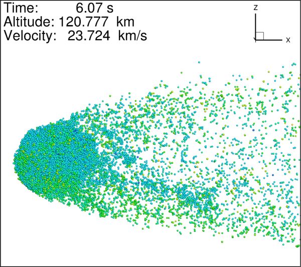
A&A 650, A101 (2021)

The heat transfer coefficient                                         Here τ denotes the luminous efficiency. The magnitude was
                                                                      obtained from the luminous intensity as M = −2.5 log I
hi j = 2k Ai j = 2k πδi j rred                                (14)
         p         p
                                                                      (Borovička et al. 2007). In a future version of our code, the
                                                                      meteor light production could be computed directly from excited
is proportional to the conductivity k of the grain material and the   electrons of ablated meteoroid molecules in the context of a rar-
contact area Ai j between two grains (Kloss et al. 2012).             efied gas flow simulation.

2.4.4. Heat loss due to mass loss                                     3. Simulation procedure
The heat consumed by meteoroid ablation is obtained as                3.1. Flow field
               ∂mi                                                    The degree of rarefaction of the atmospheric entry flow about a
qi,mass = L        ,                                          (15)
                ∂t                                                    meteoroid can be characterized by the Knudsen number Kn =
                                                                      λ/L, where λ is the mean free path length in the atmosphere and
where L denotes the heat of ablation (i.e., a combination of the      L is a characteristic length scale of the meteoroid, for instance its
heat of fusion and the heat of vaporization).                         diameter. Since a typical dustball meteoroid is in the free molec-
                                                                      ular flow regime during its entire atmospheric entry, a compu-
2.5. Mass loss                                                        tational method must be used which is able to compute highly
                                                                      rarefied gas flows. In addition, a dustball meteoroid has a
The mass loss of a meteoroid grain was modeled using                  very complex geometry, and thus flow simulations must be
the Knudsen-Langmuir and the Clausius-Clapeyron formalisms            able to handle such geometries. Thus, a recent parallel hybrid
(Campbell-Brown & Koschny 2004). The Knudsen-Langmuir                 DSMC-Fokker-Planck implementation (Gorji & Jenny 2015;
equation describes the mass loss of a grain in dependence of its      Küchlin & Jenny 2017), which is capable of simulating flows in
temperature as                                                        the whole range of Knudsen numbers and possesses the com-
                         r                                            putational efficiency to perform large-scale simulations involv-
∂mi                          µ                                        ing complex geometries, was used for the flow field simulations
     = −Ai ψ (p s − pv )            .                      (16)
 ∂t                        2πkB T i                                   around the dustball meteoroid.

Here Ai = 4πri2 is the grain’s surface area, ψ is the condensation
coefficient, which gives the probability that an evaporated mete-     3.1.1. DSMC method
oroid atom does not collide with the grain’s surface and con-         The DSMC method pioneered by Bird (1994) uses computa-
dense, µ is the average mass of a meteoroid atom, and kB is the       tional particles to simulate a rarefied gas flow. Each computa-
Boltzmann constant. The variable pv denotes the vapor pressure        tional particle represents a much larger number of atmospheric
and p s is the saturated vapor pressure which is given at a certain   molecules. Computational particles were collected in computa-
temperature by the Clausius-Clapeyron equation as                     tional cells with dimensions smaller than the local mean free
                                                                      path of atmospheric entry flow. A time step, which is smaller
                  Lµ
                      !
p s = exp K −           .                                      (17)   than the mean collision time, was used. Thus, the assumption
                 kB T                                                 is made that a computational particle can collide with any other
                                                                      particle inside the same cell regardless of its exact position. In
The constant K can be obtained by inserting a material’s boil-        addition, the assumption is made that only collisions between
ing temperature T B at sea level pressure Pa into Eq. (17), which     two particles occur. Thus, pairs of collision partners formed ran-
yields                                                                domly in each cell and the probability of their collision was com-
                                                                      puted based on the relative velocity of the two particles and their
                  Lµ
                       !
exp K = Pa exp           .                                   (18)     physical properties. The macroscopic properties of the flow were
                kB T B                                                obtained by ensemble averaging all particles in a computational
                                                                      cell. The collision between an atmospheric particle and a mete-
By combining Eqs. (16), (17), and (18) and neglecting the vapor       oroid grain was modeled purely diffusive for all DSMC compu-
pressure pv for the high altitude meteors simulated in this paper,    tations used in this paper.
the mass loss of a meteoroid grain can be expressed as a function
of its temperature as
                                                                      3.1.2. Atmospheric model
                       Lµ             Lµ
                             !              !r
∂mi                                              µ
      = −Ai ψPa exp            exp −                    .     (19)    The molecular number density in the atmosphere was obtained
 ∂t                   kB T B         kB T i    2πkB T i               using the NRLMSISE-00 model (Picone et al. 2002). Since the
                                                                      DSMC code (Küchlin & Jenny 2017) used to simulate the atmo-
2.6. Light production                                                 spheric entry flow around the meteoroid currently does not sup-
                                                                      port multispecies gas mixtures, the atmosphere was modeled as
The light production of the meteor was modeled according to           pure N2 gas with a density according to NRLMSISE-00.
the classical luminous equation (Bronshten 1983). The luminous
intensity is proportional to the mass-loss rate and the kinetic
energy of a meteoroid grain. The luminous intensity of the            3.1.3. Meteoroid ablation
meteor was obtained by summing over all grains as                     Since the Fokker-Planck-DSMC code (Küchlin & Jenny 2017)
         N                                                            does not support multiple gas species, the ablated meteoroid
         X v2 ∂mi
                i                                                     material could not be simulated in the flow field around the mete-
I = −τ                 .                                      (20)
         i=1
                2 ∂t                                                  oroid. The effect of meteoroid ablation on the flow field and the
A101, page 4 of 16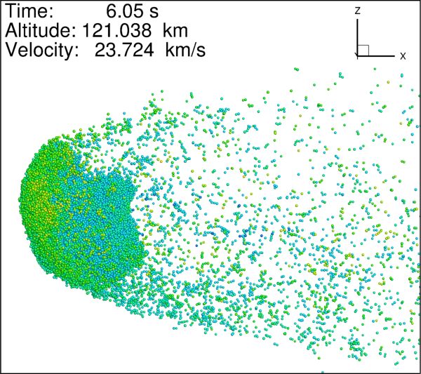
L. Hulfeld et al.: Atmospheric entry simulation of a dustball meteoroid

formation of a wake due to ablated meteoroid material should be         computationally faster version of the contact laws between adhe-
studied in the future. When air species collide at very high veloc-     sive particles, which nonetheless contains the essential physics
ities with ablated meteoroid material, dissociation and ionization      of a grain-grain interaction. As the meteoroid’s dynamics shall
reactions occur, forming an ion trail behind the meteoroid. Such        be simulated during a significant part of its flight through Earth’s
ion trails are measured by radar observations. Thus, models of          atmosphere, their contact laws were adopted here. The details of
dissociation and ionization reactions could be included in the          their method were published in Ringl & Urbassek (2012), but
Fokker-Planck-DSMC code to simulate the formation of an ion             the calculation of the contact forces and moments is repeated
trail and compare it to measured data.                                  here for convenience.
     In addition, a model of electron excitation could be included           The contact force between two grains consists of an attractive
into the code to simulate the emitted light from excited particles.     (i.e., the adhesive force), a repulsive, and a frictional part, that
This would improve the physical modeling of light emission              is
in comparison with the classical luminosity model (Bronshten
1983) used in this paper and would allow one to compute meteor          Fi j = n̂ · Fadh − Frep + t̂ · Ffric .                         (24)
spectra. These additions would result in better constraints of
meteor modeling as the computed ion trails and meteor spectra           Here, n̂ is the normal vector pointing from xi to x j and t̂ = ut /|ut |
could be compared to measurements. This would subsequently              the normal vector of the tangential velocity between the grains.
lead to a better understanding of the meteor phenomena and a            The repulsive force consisting of the Hertz force and its time
better validation of meteor models.                                     derivative to account for a viscoelastic normal contact is calcu-
                                                                        lated as
                                                                                         2 E √  3/2
                                                                                                                          !
3.2. Meteoroid dynamics                                                 Frep = max 0,
                                                                                                                   p
                                                                                                   rred δi j + Dvn δi j .                (25)
                                                                                         3 1 − v2
The main goal of this paper was to investigate disintegration-
and drag-induced rotation of a dustball meteoroid during                We note that D represents the dissipation constant, which
atmospheric entry. Thus, the simulation of the meteoroid’s              is experimentally determined and vn is the relative velocity
dynamics during atmospheric entry must include deceleration,            between two grains projected onto n. The sliding friction force
rotation, and break-up, which can be done by a single simulation        between the grains is obtained as
technique, namely the discrete element method.                                                 G
                                                                        Ffric = − min ηtang vt , πa2i j .                          (26)
                                                                                                2π
3.2.1. Discrete element method (DEM)
                                                                                                                                        E
                                                                        Here, ηtang is the tangential damping constant and G = 2(1+ν)       is
DEM pioneered by Cundall & Strack (1979) simulates the
                                                                        the shear modulus.
dynamics of each particle on the basis of external and inter-
                                                                             The contact moment between two grains has a twisting and
particle forces and moments. DEM is thus able to simulate the
                                                                        a rolling friction part. The twisting moment points in the nega-
dynamics of a meteoroid grain due to external influences and
                                                                        tive twisting direction. The twisting direction is the relative rota-
interactions with neighboring grains. For spherical grains, the
                                                                        tional velocity between two grains projected on their normal axis
governing equations of DEM have the following form:
                                                                        n̂. The rolling velocity points in the direction of the relative rota-
                        N                                               tional velocity minus the twisting velocity:
     ∂ui             X
mi       = Fi,aero +     Fi j                                   (21)
     ∂t                                                                 Mi j = Mtwist + Mroll + n̂ × t̂ · ri Ffric                        (27)
                     j=1
                                                                                                            1G 3
                                                                                                                   !
∂xi                                                                     Mtwist = − min ηtwist · |ωtwist |,      a · ω̂twist               (28)
    = ui                                                        (22)                                        3 π ij
∂t
             N

     ∂ωi X                                                              Mroll = − min ηroll · |ωroll |, 2 Fadh ξyield · ω̂roll .          (29)
Θi       =     Mi j .                                           (23)
      ∂t   j=1                                                          Here ηtwist and ηroll are damping coefficients analogous to ηtang
                                                                        used to mimic static friction. The critical rolling displacement is
Here, Fi,aero denotes the aerodynamic force acting on th ith grain.     denoted by ξyield , and ω̂twist and ω̂roll denote the unit vector of
The drag-induced aerodynamic moment was neglected. A grains             the twisting and rolling axes.
inertia tensor is denoted by Θi and the inter-particle forces and
moments by Fi j and Mi j , which are obtained based on the con-         3.3. Flow-field-DEM coupling
tact laws introduced below.
                                                                        Above, the computation of the flow field and the simulation of
3.2.2. Contact laws                                                     the meteoroid dynamics were introduced. These two methods
                                                                        were coupled, as explained below, in order to simulate the mete-
As mentioned in the introduction, the use of DEM in an                  oroid along its trajectory. The steps listed below were repeated
astrophysical context has been established recently. Thus there         until the meteoroid was fully ablated or disintegrated.
are a number of contact laws proposed by different authors                  The current meteoroid geometry and atmospheric density
for the use of adhesive particles in DEM, for example,                  were used to perform a stationary simulation of the flow field
in work done by Luding (2008), Wada et al. (2007, 2008),                around the meteoroid and obtain Fi,aero and qi,conv for each grain
and Dominik & Nübold (2002). However, their contact laws                and to compute the view factors Fi→ j between all meteoroid
rely on very detailed implementations of the physics of                 grains. On the basis of these stationary computations a transient
grain-grain interaction, which makes them computationally               simulation of the meteoroid was carried out. The dynamics of
expensive and restricts the number of computational parti-              each grain initiated by the aerodynamic force Fi,aero were cal-
cles. Recently, Ringl & Urbassek (2012) proposed a simplified,          culated by means of the DEM by solving Eqs. (21)–(23). Then
                                                                                                                            A101, page 5 of 16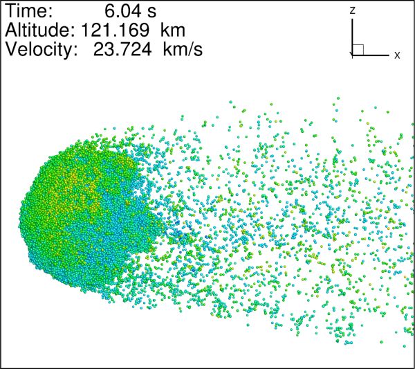
A&A 650, A101 (2021)

the heat transfer was computed according to Eq. (10), using the                                  Earth-fixed system
stationary view factors Fi→ j , and the mass loss of each grain was              zE
calculated according to Eq. (19). In addition, the meteoroid’s
trajectory was also calculated. During the transient part of the                  (0, 0, h0 )E
simulation, the termination conditions introduced below were                               xE
checked continuously to determine if new flow field and view                yE
                                                                                      zR                   Meteoroid trajectory
factor computations are needed.
    The displacement of each grain was tracked during the tran-
sient simulation as dxi = |xi − xi,0 |. Here, xi denotes a grain’s cur-                                           zM
rent position and xi,0 is the grain’s position at the time the flow                                        xM
field and view factor computations were carried out. The fol-                                                    (0, 0, 0) M
lowing three termination conditions were introduced in order to                                             yM
guarantee that the flow field around the meteoroid and the view                                                        v0
factors between the individual meteoroid grains did not change
too much during a transient simulation step.
    Firstly, the standard deviation of the grains’ displacements                                         Moving system
dx has exceeded its threshold value. Secondly, the atmospheric
density as calculated by the NRLMSISE-00 model has changed
by a certain amount. Thirdly, the meteoroid’s velocity (i.e., the
velocity of the fastest grain) has changed by a certain amount.
If one of these termination conditions was fulfilled, the current                                       EARTH SURFACE
transient simulation step was terminated and new atmospheric
entry flow and view factor computations were carried out.                 Fig. 1. Sketch of Earth-fixed coordinate system and moving system used
                                                                          during the simulation of a dustball meteoroid’s atmospheric entry.

3.4. Coordinate systems
                                                                                                                                     zM
During the transient simulation steps, two different coordinate
systems were used. An Earth-fixed coordinate system was used
to calculate the trajectory of the meteoroid and a meteoroid-                                                                                 xM
fixed coordinate system was used to calculate the dynamics of                                                                      yM
the meteoroid. Both coordinate systems are sketched in Fig. 1.
                                                                                                                                  Grain outside
                                                                             d                                                    domain
3.4.1. Earth-fixed system
The Earth-fixed system is defined such that its z-coordinate zE                                                                Simulation
points away from the center of the Earth, that is to say the                                                                   domain
gravitational force acts in the negative z direction. Its x-axis xE
is defined such that the trajectory of the meteoroid lies in the                  Meteoroid
xz-plane of the Earth-fixed system. The origin of the Earth-fixed
coordinate system is defined by the projection of the meteoroid’s
position at the start of the simulation onto the Earth surface. At
the start of the simulation, the meteoroid’s position is given in                                   L
the Earth-fixed system as (0, 0, h0 )E and its initial velocity by u0 .
                                                                          Fig. 2. Sketch of the simulation domain.

3.4.2. Moving system
                                                                          the frond side of the simulation domain is chosen such that the
The moving coordinate system was used to calculate the dynam-             inflow conditions are defined properly and a possible bow shock
ics of each meteoroid grain with DEM and the atmospheric entry            is located inside the simulation domain. All grains, which are
flow about the meteoroid. The free atmospheric entry stream               currently located within the simulation domain, were simulated
flows in positive x M -direction. The origin of the moving sys-           using the coupling procedure between DEM and Fokker-Planck-
tem is initially located in the Earth-fixed system at (0, 0, h0 )E .      DSMC introduced above. Grains, which have left the simulation
The moving system moves with a constant speed v0 and radi-                domain, can be simulated as described in Sect. 5. A grain which
ant zenith distance cos (zR ) through Earth’s atmosphere, cor-            has left the simulation domain is not allowed to reenter again.
responding to a non-decelerated meteoroid. Thus, the moving
system’s origin at time t is represented by (v0 sin (zR ) t, 0, h0 −
v0 cos (zR ) t)E in the Earth-fixed system. The moving system’s           4. Simulating the atmospheric entry of a Draconid
orientation is such that its x-axis x M is opposed to u0 .                   meteoroid
                                                                          To test and validate the meteoroid model and the simulation
3.4.3. Simulation domain                                                  procedure introduced above, a Draconid meteoroid was chosen.
                                                                          Firstly, Draconids were chosen since they represent some of the
The simulation domain is defined by a cubic box in the moving             most fragile and porous meteoroids the Earth encounters. They
coordinate system as sketched in Fig. 2. The simulation domain            are often used in the literature as prototype dustball meteoroids.
has a certain size L. The distance d between the meteoroid and            Secondly, Draconid meteoroids enter Earth’s atmosphere at a

A101, page 6 of 16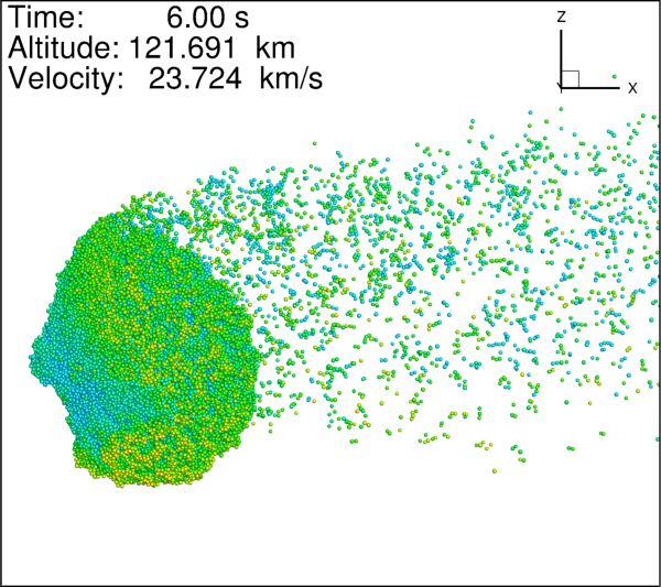
L. Hulfeld et al.: Atmospheric entry simulation of a dustball meteoroid

Table 1. Material properties employed to model a Draconid meteoroid.

           Material property                 Symbol        Value          Unit                        References
           Grain density                     ρGrains       3000          kg m−3            Borovička et al. (2007) (1)
           Young modulus                        E        54 · 109          Pa             Ringl & Urbassek (2012) (2)
           Poisson ratio                        ν          0.17                           Ringl & Urbassek (2012) (2)
           Surface tension                      γ         0.014           J m−2              Heim et al. (1999) (3)
           Critical rolling displacement      ξyield    32 · 10−10          m                Heim et al. (1999) (3)
           Specific heat capacity              cp          1000        J kg−1 K−1     Campbell-Brown & Koschny (2004) (4)
           Conductivity                         k            3         W m−1 K−1      Campbell-Brown & Koschny (2004) (4)
           Boiling temperature                 TB          2100             K         Campbell-Brown & Koschny (2004) (4)
           Condensation coefficient             ψ           0.5                       Campbell-Brown & Koschny (2004) (4)
           Average atomic mass                  µ           23             a.u.       Campbell-Brown & Koschny (2004) (4)
           Specific heat of ablation            L        3.5 · 106       J kg−1       Campbell-Brown & Koschny (2004) (4)
           Emissivity                                       1

relatively low speed of 24 km s−1 . At such low speeds, sputter-        2.5, and an initial meteoroid mass of m0 = 1.35 · 10−5 kg
ing of the meteoroids could be neglected and the mass loss can          were used. The Draconid’s porosity was assumed to be 90%
be modeled exclusively by thermal ablation (Popova et al. 2007)         (Borovička et al. 2007). The meteoroid’s initial geometry is pre-
since our code is currently not able to simulate sputtering.            sented in Fig. 3a. The meteoroid’s shape was assumed to be per-
                                                                        fectly spherical.
4.1. Modeling a Draconid meteoroid
The code used to simulate the flow field about the meteoroid            4.2. Simulation parameters
(Küchlin & Jenny 2017) is currently not able to simulate ablated
meteoroid material. Therefore, a meteoroid which stays in the           The following parameters were used in the simulation of the Dra-
free molecular flow regime during its entire flight through             conid’s atmospheric entry.
Earth’s atmosphere should be selected.
                                                                        4.2.1. Initial conditions
4.1.1. Reference Draconid                                               It was found that for typical Draconid speeds around 24 km s−1 ,
The Draconid meteor no. 96 measured by Borovička et al.                the forces and heat fluxes above 200 km are small enough not to
(2007) was selected as a reference for the simulation presented         lead to meteoroid disintegration shortly after the start of the sim-
here. The first reason to select this meteoroid is given by the         ulation. Nevertheless, the forces at an altitude of 200 km were
fact that it is small enough to remain in the free molecular flow       big enough to trigger meteoroid deformation right after the start
regime during its entire flight through the atmosphere. The mean        of the simulation, as can be seen in Fig. 3. Since our simulation
free path length at 100 km, where this meteoroid disintegrates, is      was computationally very expensive, we decided not to start the
14 cm and the Draconid’s diameter was measured to be 4.5 mm,            simulation at a higher altitude than h0 = 200 km.
which results in a Knudsen number of 31. However, the Knudsen               The meteoroid’s initial velocity v0 at this altitude was
number could be lower if meteoroid ablation was modeled.                obtained by extrapolating the measured velocity of meteor No.
    Secondly, this meteoroid was selected because the number            96 (Borovička et al. 2007) to an altitude of 200 km. Thus, v0 =
of grains proposed by Borovička et al. (2007) is small enough to       23.73 km s−1 was obtained. The Draconid’s direction of travel,
enable a fast simulation. Simulations of larger meteoroids with         defined by its cosine of the radiant zenith distance (cos (zR ) =
hundreds of thousands of grains would be possible too, but that         0.55), was adopted from the same source.
would lead to unacceptably high simulation times.                           The assumption was made that the Draconid has no initial
                                                                        rotation, which is very unlikely as most celestial bodies are rotat-
4.1.2. Material properties                                              ing. In addition, millimeter-sized meteoroids experience drag-
                                                                        induced rotation during ejection from their parent comet (Čapek
Since no exact material parameters are known for Draconids, and         2014). The procedure introduced in Sect. 3 is able to simulate
since different Draconids may even have different material prop-        drag-induced meteoroid rotation during atmospheric entry. The
erties depending on their origin within the parent comet, certain       meteoroid’s drag-induced rotation is presented in Sect. 4.3.2.
Draconid material properties had to be assumed. The mechani-
cal properties of SiO2 were used during the simulation, and black
                                                                        4.2.2. DSMC parameters
body radiation was assumed. The material parameters used in the
simulation together with the sources where they were taken from         A parameter study of the flow field around the meteoroid was
are presented in Table 1.                                               carried out to obtain the size of the simulation domain and the
                                                                        number of particles in the domain. Due to computational con-
4.1.3. Meteoroid geometry
                                                                        straints, it was important for the purposes of this parameter study
                                                                        to find a minimal simulation domain and the smallest number of
To model the meteoroid, the procedure introduced in Sect. 2.3           particles which still allow one to simulate the atmospheric entry
was employed. Upper and lower grain masses of mu = 5.5 ·                flow. The goal of the parameter study was to obtain smooth heat
10−10 kg and ml = 2.8 · 10−10 kg, a power law index of s =              fluxes and aerodynamic forces acting on the meteoroid grains.

                                                                                                                         A101, page 7 of 16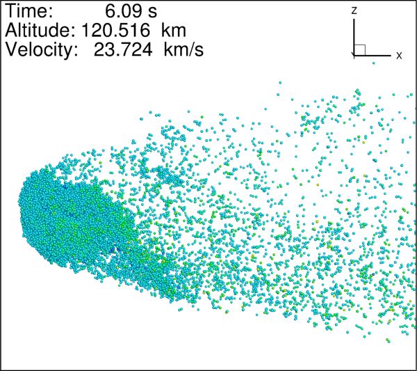
A&A 650, A101 (2021)

                       (a)                                               (b)                                               (c)

Fig. 3. Meteoroid before (a) and after (b) compression at about 200 km and a cut through the meteoroid at 135 km (c). The atmospheric entry flow
is directed in the positive x-direction, while the meteoroid moves in the opposite direction. The radiant zenith distance of the meteoroid’s direction
of flight is zR = 56.6◦ .

    It was found that the distance s between the meteoroid and                 temperature distribution is presented below. The motion of the
the front side of the simulation domain should have a mini-                    meteoroid grains after disintegration and the resulting meteor
mum size of 1 mm to properly resolve the inflow conditions and                 plots (i.e., light curve, deceleration curve, etc.) are presented in
that a total number of 2 million particles is sufficient to obtain             Sect. 5.
smooth enough forces and heat fluxes. The length of the simula-
tion domain L was set to 10 cm. This ensures that a grain, which
has left the simulation domain, has separated from the remaining               4.3.1. Meteoroid deformation
meteoroid grains enough to justify the assumption of free flow                 Figure 3a shows the initial meteoroid geometry at the start of
about that grain.                                                              the simulation at a 200 km altitude. The aerodynamic forces are
                                                                               small at this altitude, but they are able to deform the meteoroid
4.2.3. DEM parameters                                                          within the first 0.17 s of the simulation. Meteoroid deformation
                                                                               occurs due to rolling between grains since rolling only requires
For the DEM part of the simulation, a time step size of dtDEM =                small aerodynamic forces. During compression of the mete-
10−9 s was found to be small enough to accurately resolve the                  oroid, not a single bond between grains is broken, but many new
forces between meteoroid grains. On the basis of this time step,               grain bonds form due to collisions with subcritical velocities.
the damping coefficients were determined.                                      The meteoroid geometry after compression at 0.17 s is shown
      The dissipation coefficient A was determined such that two               in Fig. 3b. The meteoroid deformation depends on the rolling
50 µm grains stuck together after a normal collision with their                forces, which depend on the surface tension γ and the critical
critical sticking velocity vcrit = 0.17 m s−1 (Blum & Wurm                     rolling displacement ξyield . If a higher value of ξyield was chosen,
2000). This leads to A = 3·10−7 s. The damping coefficients ηtang ,            meteoroid compression might not have started at 200 km since
ηroll , and ηtwist depend on the time step size dtDEM . The tangen-            the aerodynamic forces probably would have been too small. But
tial damping coefficient ηtang = 2.5 · 10−2 kg s−1 was determined              most certainly the meteoroid would have been compressed, nev-
in a test simulation. The other damping coefficients were chosen               ertheless, just at a lower altitude. In order to investigate whether
in agreement with Ringl & Urbassek (2012) as ηroll = ηtwist =                  meteoroid compression would happen if a higher critical rolling
0.4ri2 ηtang as a function of a grain’s radius ri .                            displacement was chosen, another simulation with a higher ξyield
                                                                               is required.
4.2.4. Coupling parameters                                                          After compression, the meteoroid’s porosity decreases from
                                                                               90% to about 80% since the meteoroid was compressed to
The following termination conditions were employed to couple                   roughly half its volume. The meteoroid’s structure is much stiffer
the flow field and DEM computations throughout the Draconid’s                  now and there is no more deformation and rolling between mete-
atmospheric entry simulation. The changes in atmospheric den-                  oroid grains. This increased meteoroid stiffness results from a
sity and meteoroid velocity were both set to 5%. A threshold                   higher number of grain bonds, which makes it harder for grains
value of 50 µm was used for the standard deviation of meteoroid                to roll on each other. The simulation results show that after initial
grain displacements.                                                           compression, the meteoroid keeps the same shape and orienta-
                                                                               tion until an altitude of 155 km. At 155 km, the meteoroid begins
4.3. Results                                                                   to rotate due to slightly asymmetric aerodynamic forces. After
                                                                               compression and until disintegration of the meteoroid at 123 km,
The following section presents the results of the coupled sim-                 the meteoroid nearly behaves as a rigid body. Below 123 km, the
ulation with the parameters introduced above. The deforma-                     aerodynamic forces grow big enough to trigger rolling between
tion and motion of the meteoroid during its travel through                     grains, which leads to further deformation of the compressed
Earth’s atmosphere is described until the meteoroid is fully                   meteoroid. The subsequent disintegration of the meteoroid is dis-
disintegrated at about 120 km. Additionally, the meteoroid’s                   cussed below.

A101, page 8 of 16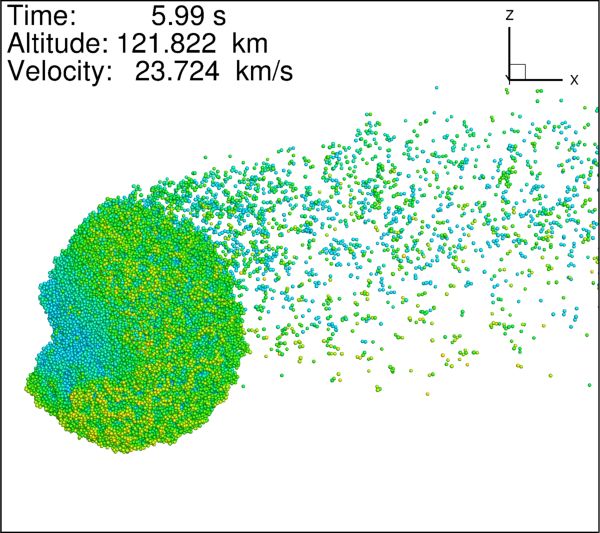
L. Hulfeld et al.: Atmospheric entry simulation of a dustball meteoroid

                                                                         aerodynamic forces are actually smaller than adhesive forces,
                                                                         but they are big enough to trigger significant rolling motion
                                                                         of grains in the compressed meteoroid. At 123 km, this leads
                                                                         to many grain collisions which are above the critical velocity.
                                                                         Super-critical collisions often lead to the separation of exist-
                                                                         ing grain bonds. Separated grains may further collide with other
                                                                         meteoroid grains, which further triggers the break-up of grain
                                                                         bonds for super-critical collisions. On the other hand, subcrit-
                                                                         ical collisions lead to the formation of new grain bonds. Due
                                                                         to super-critical collisions, grains continue to separate from the
                                                                         meteoroid. Figure 5 shows that the meteoroid continuously dis-
                                                                         integrates from the outside in. The meteoroid disintegrates into
                                                                         small pieces of only a couple of grains. There is no such thing as
                                                                         a sudden break-up or fracturing of the meteoroid into a couple of
                                                                         big pieces. According to our simulation, the meteoroid is almost
                                                                         fully disintegrated at an altitude of 120 km. The break-up occurs
                                                                         over a 3 km altitude span due to super-critical grain collisions,
Fig. 4. Meteoroid rotation frequency from the start of the simulation    which are triggered by aerodynamically-induced rolling motion.
until the start of meteoroid disintegration.
                                                                             The temperature of the grains is too low for significant
                                                                         ablation. Compared to the reference Draconid, which started to
4.3.2. Drag-induced meteoroid rotation
                                                                         disintegrate at 102 km, the Draconid in our simulation started
In Fig. 4, we can see the meteoroid’s rotational frequency from          disintegrating 21 km earlier. Since break-up was initiated by the
the start of the simulation until the beginning of meteoroid break-      rolling motion between grains, a higher critical rolling displace-
up. We can see that the meteoroid begins to rotate at about              ment ξyield should be selected in order to correct for the mismatch
155 km. Above this altitude, the aerodynamic forces acting on            in the disintegration height. In that case, however, ablation may
the grains were too small to induce meteoroid rotation. Below            become relevant since there is more time to heat up the grains. A
155 km, the meteoroid begins to rotate faster and faster until           more detailed discussion about dustball break up mechanisms,
it begins to break apart at about 123 km. Our simulation shows           based on out simulation framework, can be found in Sect. 6.8.
that even for a pretty symmetrical meteoroid drag-induced mete-              In Fig. 5, one can see that grains around 600 K from the
oroid, rotation occurs at a relatively high altitude of 155 km.          front of the meteoroid separated together with cold grains around
Thus we can conclude that for a real nonsymmetrical meteoroid,           350 K from the back of the meteoroid. If thermal meteoroid dis-
drag-induced rotation plays an important role. Figure 3c shows           integration occurs, only grains which have a high enough tem-
the meteoroid at 135 km, and it can be seen that the meteoroid is        perature would separate themselves from the meteoroid. This
rotating. In Fig. 5, we can see the meteoroid during disintegra-         would probably lead to an increased disintegration duration. In
tion between 123 and 120 km. We can see that the meteoroid still         addition, separated grains would instantaneously ablate, while
is rotating during disintegration, although it no longer behaves         the remaining meteoroid grains would need to heat up first
similar to a rigid body.                                                 before they separate. This results in a light curve which looks
                                                                         more like that of a typical dustball meteor (see Sect. 5.2).
4.3.3. Meteoroid temperature
Figure 3c shows a cut through the middle of the meteoroid at             4.3.5. Number density distribution
135 km. We can see that the meteoroid still has the same shape           In Fig. 6, the grain number density distribution at the end of our
as at 197 km after compression and that it is rotating. The pic-         simulation is presented. The coupled DEM-DSMC simulation
ture shows the temperature distribution of the meteoroid after           was terminated at 119 km after almost every grain had separated
5 s of simulation time. We can see that only a small outer layer         from any other meteoroid grain. The figure shows that the mete-
has reached a temperature of 550–450 K. Then there is a layer            oroid grains are not distributed symmetrically about the x-axis.
of grains between 450–350 K and the meteoroid’s core has only            This is due to meteoroid rotation occurring before and during
reached temperatures of 350–300 K. This is due to the fact that          disintegration.
for most of the time, the front part of the meteoroid has been               Grains which separated earlier have already been decelerated
exposed to atmospheric entry flow and thus it received most              more than grains which separated later. Thus, a small physical
of the thermal energy. We note that the dominant heat transfer           wake of approximately 2.5 m length has formed. The meteoroid
mechanism inside the meteoroid is radiation. Conduction and              grains are distributed equally in space as a function of their mass
convective heat transport between meteoroid grains are negligi-          since there was not enough time to separate them due to atmo-
ble since contact surfaces between grains and atmospheric den-           spheric deceleration.
sity are very small. Figure 5 shows that after the disintegration
of the meteoroid’s outer layer which had a temperature of about
600 K, the core of the meteoroid still had a temperature of only         5. Simulating grain ablation after meteoroid
350–400 K.
                                                                            disintegration

4.3.4. Meteoroid disintegration                                          After a grain has separated from the meteoroid by a suffi-
                                                                         ciently large distance, it can be simulated independently of all
In Fig. 5, we can see how the meteoroid disintegrates. We can            other meteoroid grains. Therefore the aerodynamic force and the
also see meteoroid rotation during disintegration. At 123 km,            incoming atmospheric heat flux acting on a separated meteoroid
                                                                                                                         A101, page 9 of 16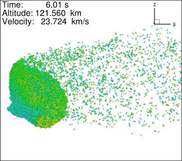
A&A 650, A101 (2021)

Fig. 5. Meteoroid during disintegration. The radiant zenith distance of the meteoroid’s direction of flight (-x-axis) is zR = 56.6◦ .

A101, page 10 of 16
L. Hulfeld et al.: Atmospheric entry simulation of a dustball meteoroid

Fig. 6. Two dimensional number density distribution of the meteoroid grains after full disintegration at an altitude of 119 km.

are obtained according to                                                  Eq. (10) and neglecting radiative heat transfer with any other
                                                                           grain, the following equations were obtained:
Fi,aero = −ΓS i ρa v2i · ûi and                                   (30)                        v3
                                                                                ∂T i                                         ∂mi
                    v3i                                                    c p mi     = ΛS i ρa i + σAi (T env
                                                                                                              4
                                                                                                                − T i4 ) + L            (34)
qi,conv = ΛS i ρa         .                                        (31)          ∂t             2                             ∂t
                    2                                                                              Lµ             Lµ
                                                                                                         !              !r
                                                                           ∂mi                                                  µ
                                                                                 = −Ai ψPa exp             exp −                      . (35)
                                                                             ∂t                   kB T B         kB T i      2πkB T i
Here, S i = πri2 denotes the cross section of the grain, Λ is the
heat transfer coefficient, Γ is the drag coefficient, ρa is the atmo-      We note that for separated meteoroid grains, these equations
spheric density, vi is the grain’s absolute velocity, and ûi is the       can be employed and neither DEM nor DSMC simulations
unit vector of the grain’s velocity.                                       should be performed any more. Thus calculating grain abla-
    The dustball meteoroid which was used in the simula-                   tion after meteoroid disintegration was computationally very fast
tion was modeled on the basis of meteor no. 96 presented in                and thus allowed for us to optimize certain model parameters in
Borovička et al. (2007). The biggest diameter of any grain in this        order to better fit measurements of the reference Draconid from
meteoroid model is 70 µm. Borovička et al. (2007) reported that           Borovička et al. (2007).
the corresponding meteoroid was fully ablated at an altitude of
93 km, where the mean free path in the atmosphere is 41 mm,                5.2. Light curve
which results in a Knudsen number of Kn = 585. Thus, even if               Using the mass loss rate of each meteoroid grain according to
grain ablation is taken into account, every separated meteoroid            Eq. (35), the meteor’s luminous intensity and its magnitude were
grain is clearly in the free molecular flow regime. Therefore, a           calculated as explained in Sect. 2.6. The meteor’s magnitude was
heat transfer coefficient of Λ = 1 and a drag coefficient of Γ = 1         plotted to obtain its light curve. This fit, together with the mea-
were used during the entire grain ablation simulation.                     sured light curve and the erosion model fit by Borovička et al.
                                                                           (2007), is presented in Fig. 7.
5.1. Ablation model                                                            As one can see from Fig. 7, the resulting light curve, using
                                                                           the material properties from Table 1 (i.e., L = 3.5 · 106 J kg−1 ),
When a meteoroid grains have separated by a sufficiently large             does not match the reference from Borovička et al. (2007) very
distance, the equations introduced above are used to calculate a           well. The meteoroid starts to ablate at 118 km, that is to say
grain’s aerodynamic force and heat flux.                                   shortly after disintegration. First, the light curve looks like that
    Thus, the trajectory of a grain can be calculated according to         off a dustball, but from 116 km on it has the shape of a clas-
                                                                           sical single body light curve. This is due to the fact that after
  ∂ui                                                                      separation, there is no more shielding of meteoroid grains and
mi    = −ΓS i ρa v2i · ûi and                                     (32)
   ∂t                                                                      every grain receives the full heat flux from the free atmospheric
∂xi                                                                        entry flow. At 116 km, nearly every grain is heated up to around
    = ui .                                                         (33)    800 K. Since all meteoroid grains have the same temperature,
∂t
                                                                           they all ablate around the same time, thus producing a classi-
The ablation of a separated meteoroid grain was calculated                 cal single body light curve below an altitude of 116 km. Further,
similarly to grain ablation during the DEM-DSMC simulation,                using a specific heat of ablation of L = 3.5 · 106 J kg−1 caused the
as presented in Sects. 2.4 and 2.5. By inserting Eq. (31) into             meteoroid to ablate too early.
                                                                                                                              A101, page 11 of 16
A&A 650, A101 (2021)
Fig. 7. Resulting light curves based on the results of our DEM- Fig. 8. Deceleration curve based on our simulation results, using a heat
DSMC simulation. Measurements and erosion fit of meteor No. 096 of ablation value of L = 13.7 · 106 J kg−1 compared to measurements
by Borovička et al. (2007) compared to our light curves, computed for and the erosion fit of meteor No. 096 by Borovička et al. (2007).
three different values of heat of ablation.
Since thermal disintegration played no role, the simulation
presented in Sect. 4.3 could also be carried out using a higher
specific heat of ablation. The specific heat of ablation of L =
3.5 · 106 J kg−1 (Campbell-Brown & Koschny 2004) is one of the
lowest values found in the literature; the highest one reported for
Draconids is L = 25.0 · 106 J kg−1 (Borovička et al. 2007). Using
this specific value results in the respective light curve presented
in Fig. 7. One can see that the start of the light curve matches
the measurements pretty well; there are significant discrepancies
for the rest of the curve, however. The peak of the light curve is
about 6 km lower and the magnitude is one order too small. The
shape of the light curve looks like a typical symmetrical dustball
light curve.
The lowest L-value leads to a light curve which occurs ear-
lier than the measured one, and the highest L-value leads to a
later onset. Thus, a value between the minimum and maximum
heat of ablation values found in the literature should produce a
better fit with observations. Therefore, a fitting procedure was
performed to obtain the best match between the simulation and
observations. The fitting procedure led to L = 13.7 · 106 J kg−1 , Fig. 9. Time height intensity scan computed from the results of the cou-
and the resulting light curve is shown in Fig. 7. The start of the pled simulation.
light curve is 6 km too high and from 108 to 102 km it does not
match observations at all. Also the shape of this light curve looks
more like a classical light curve rather than that of a dustball.
5.4. Time height intensity scan
However, from 102 km on, it fits measurements pretty well and,
therefore, this heat of ablation value was adopted to produce the Based on the results presented in the previous section, a time
plots shown in the remainder of this section. height intensity scan was computed. We can see in Fig. 9 that
the time height intensity scan is very thin in the beginning of
5.3. Deceleration curve the trajectory and gets bigger towards the end of the trajectory.
Moreover, the end of the trajectory is blurred significantly. This
Using the luminous intensity of each grain, the deceleration of artificial time height intensity scan compares very well
the meteoroid was calculated. The meteor’s deceleration was cal- with the Draconid time height intensity scans presented in
culated as the height difference between the brightest meteoroid Borovička et al. (2007). In the final part of the trajectory, one
point (i.e., the highest magnitude grain) and the non-decelerated can also see the deceleration of the Draconid meteoroid since the
meteoroid (using the velocity of the brightest grain at 102 km time height intensity scan is no longer a straight line, but it bends
altitude). This deceleration is plotted in Fig. 8 together with mea- upwards. For dustball meteoroids similar to Draconids, it is typ-
surements of meteor no. 96 and the erosion fit by Borovička et al. ical that one can see the deceleration in the time height intensity
(2007). We can see that our model agrees well with the measured scan; this is in contrast to single body meteoroids, which produce
deceleration below an altitude of 97 km. a straight line.
A101, page 12 of 16L. Hulfeld et al.: Atmospheric entry simulation of a dustball meteoroid
Fig. 11. Length of the meteor’s physical wake.
Fig. 10. Meteor trail intensity at three different points of the trajectory:
at the beginning of the trajectory (Height = 107.5 km), at the point of 5.6. Wake length
highest magnitude (Height = 97.0 km), and at the end of the trajectory The meteor’s wake length is shown in Fig. 11. One can see that
(Height = 90.5 km).
the meteor produces a physical wake of up to 800 m near the
end of its trajectory. The longest trail lengths for dustball mete-
ors found in the literature (Armitage & Campbell-Brown 2020;
5.5. Meteor trail intensity Campbell-Brown et al. 2013) are around 450 m, which is some-
The meteor’s trail intensity is shown in Fig. 10 at the following what shorter than what we predicted with our simulation. On the
three different points along the trajectory: at the beginning, at other hand, the wake lengths from Armitage & Campbell-Brown
the point of highest magnitude, and at the end of the trajectory. (2020) and Campbell-Brown et al. (2013) were taken at loca-
If one compares the computed trail intensity at the beginning tions of higher magnitudes, where our simulation produces
of the meteor (107.5 km altitude) with measurements of dustball comparable wake lengths. In addition, it also must be noted
meteor trail intensities from Campbell-Brown et al. (2013) and that trail intensities and wake lengths are largely based on
Armitage & Campbell-Brown (2020), one can see good agree- the grain size distribution, and not only on the disintegration
ment. The trail intensity at an altitude of 107.5 km consists of a details.
short peak ∼40 m in length. This agrees well with the measured
trail intensities at the beginning of meteor light curves shown in
Armitage & Campbell-Brown (2020). 6. Discussion
The relative luminous intensity along the trail at peak 6.1. Coupling procedure
magnitude is also plotted in Fig. 10. A comparison to
measured trail intensities (Armitage & Campbell-Brown 2020; In the simulation presented in this paper, meteoroid and fluid
Campbell-Brown et al. 2013) shows bad agreement. The mea- dynamics were loosely coupled. In each time step, first a station-
sured trail intensities peak at the beginning and decrease towards ary DSMC computation about the meteoroid was carried out,
the end of the trail. The computed trail intensity at peak mag- and then the meteoroid dynamics was computed using constant
nitude, however, increases constantly with an increasing trail aerodynamic forces acting on each grain. Future improvement
distance. This effect is due to the fact that lighter particles of the simulation framework could include a tighter coupling
decelerate faster than heavier particles and to the power law between meteoroid and fluid dynamics, and maybe even direct
distribution of meteoroid grain masses, which ensures that the coupling. Of course, there is a trade-off between computational
meteoroid consists of more lighter grains. Similar increasing efficiency and temporal accuracy. In the simulation presented in
trail intensities could also be observed in some of the mod- Sect. 4.3, a total of about 5’000 DSMC computations were car-
eled dustballs presented in Campbell-Brown et al. (2013), which ried out. The time step sizes between two consecutive DSMC
used power law distributions. If another grain distribution (e.g., computations varied greatly since they were largely determined
Gaussian) were chosen, other trail intensities would result. We by meteoroid deformation. Thus, much smaller time steps were
can see that the trail at peak magnitude has a length around used during meteoroid disintegration than at the point of the tra-
200 m. jectory where the compressed meteoroid behaved like a rigid
The trail intensity at the lowest computed height of 90.5 km body.
can also be found in Fig. 10. We can see that it increases steeply
at the beginning and is almost constant in the rest of the trail. 6.2. Flow field
The trail length is much bigger with over 800 m. This increase in
trail length is due to the fact that grains lose mass during ablation In the flow field simulations of this paper, a pure N2 -atmosphere
and thus the remaining grains get even smaller, leading to larger was considered. If a multispecies model was used, the com-
separation due to higher atmospheric deceleration. position of the atmospheric gas could be modeled more
A101, page 13 of 16You can also read