Shanna Chu, comparison of spectral decomposition & eGf spectral ratio methods - Southern California Earthquake Center
←
→
Page content transcription
If your browser does not render page correctly, please read the page content below
Shanna Chu, comparison of spectral decomposition
             & eGf spectral ratio methods
       -    Data is pre-processed using the same selection criteria: window length, SNR above 3 in 10
            frequency bands 1-40 Hz, P-wave
       -    For one method, I performed spectral decomposition with post-inversion constraint of the event
            spectra to a spatially-varying correction function derived from pinning stacked events in 0.2
            magnitude bins to a Brune model.
       -    For the second method, I performed spectral ratios using an empirical Green’s function. The eGfs
            are selected to be within 1 source radius of the target events (preliminarily calculated with 2.4 MPa
            stress drop) and minimum cross-correlation coefficient of 0.5.
       -    For spectral ratios, deviation from the Brune spectrum can be used to obtain peak-to-peak ratio, a
            proxy for source complexity which has variation across stations. The difference between GIT
            spectra (which uses all stations for an event) also shows a station-by-station difference to the
            spectral ratios.

                             Shanna Chu
                               USGS
                           schu@usgs.gov

1/26/2023                                    Southern California Earthquake Center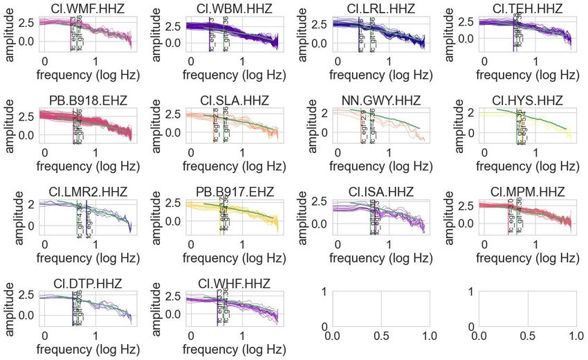
F_c ~ 4.3 with GIT and 2.9-5.7 Hz with eGf method. The   Chu
two methods are closest at PB (borehole) stations.

                                                     2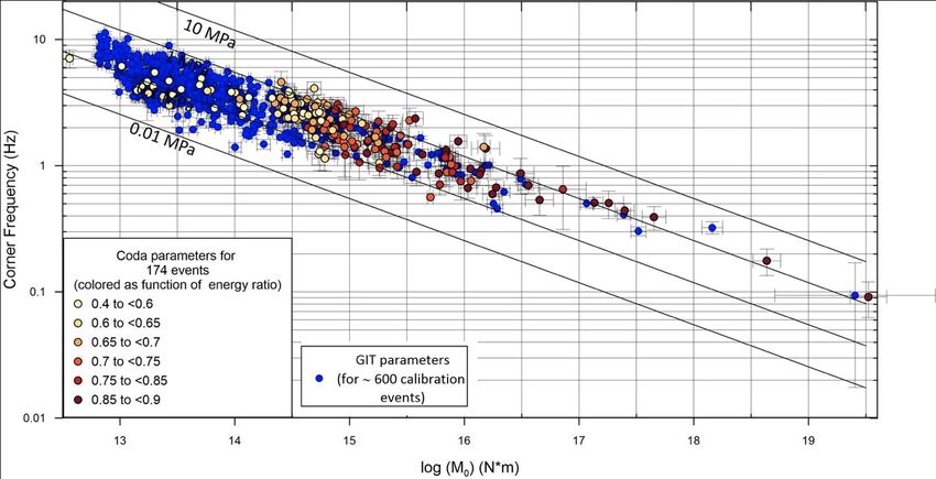
Some more figures, results, discussion       Chu

                                         3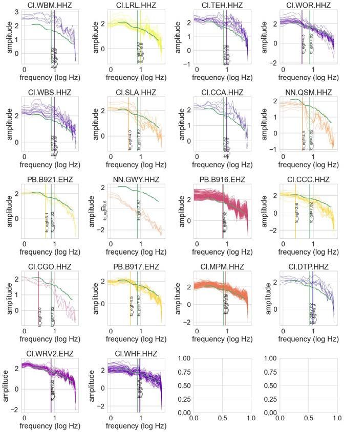
Chu
           EXTRA SLIDES

38445975 M4.04 GIT fc=4.36 sd=25.04 MPa
38445975 M4.04 eGf fc=3.03 sd=6.58 MPa
38451079 M4.09 GIT fc=8.21 sd=104.58 MPa
38451079 M4.09 eGf fc=2.44 sd=4.07 MPa
38471103 M3.3 GIT fc=12.84 sd=18.76 MPa
38483215 M3.02 GIT fc=10.77 sd=8.09 MPa
38538991 M4.13 GIT fc=7.82 sd=79.01 MPa
38538991 M4.13 eGf fc=7.51 sd=136.3 MPa
38489543 M2.54 GIT fc=10.61 sd=1.97 MPa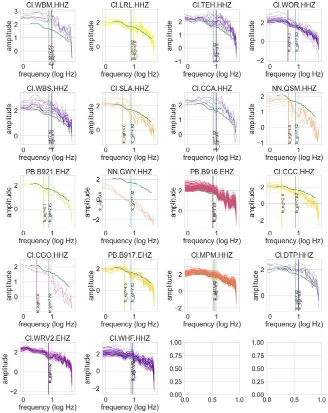
Trey Knudsen and Bill Ellsworth
   Measuring Source Parameters using Peak Amplitudes
      ●      We measure the seismic moment and corner frequency of earthquakes using narrow band filtered peak displacement
             amplitudes. Errors are assessed using the bootstrap.
      ●      “Richter”-like frequency dependent attenuation curves are used to correct for geometric spreading and anelastic loss.
      ●      We have also estimated station corrections to the attenuation curves. These may account for path differences, site
             differences and radiation pattern.
      ●      Results reveal a strong covariance of seismic moment and corner frequency.

                           Trey Knudsen                                                         Bill Ellsworth
            Department of Geophysics Stanford University                         Department of Geophysics Stanford University
                       trey05@stanford.edu                                               wellsworth@stanford.edu

1/26/2023                                           Southern California Earthquake Center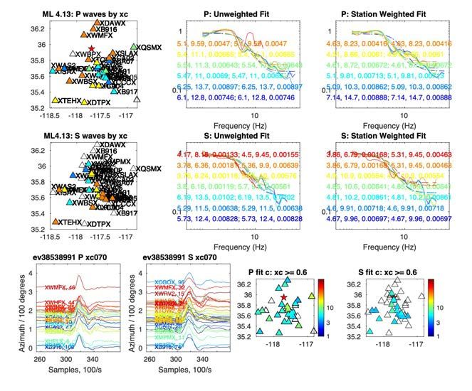
July 5 00:18 Mcat 4.04 ID 39445975                                                    Knudsen and
                                                                                        Ellsworth
  Mw 4.06, stress drop 9.0 MPa, fc 1.65 Hz

      Measured amplitudes

                             Best-fitting Brune spectrum
                             With bootstrap analysis                 Misfit error analysis
      Corrected amplitudes                                           Note covariance between seismic moment
                                                                     and corner frequency

1/26/2023                    Southern California Earthquake Center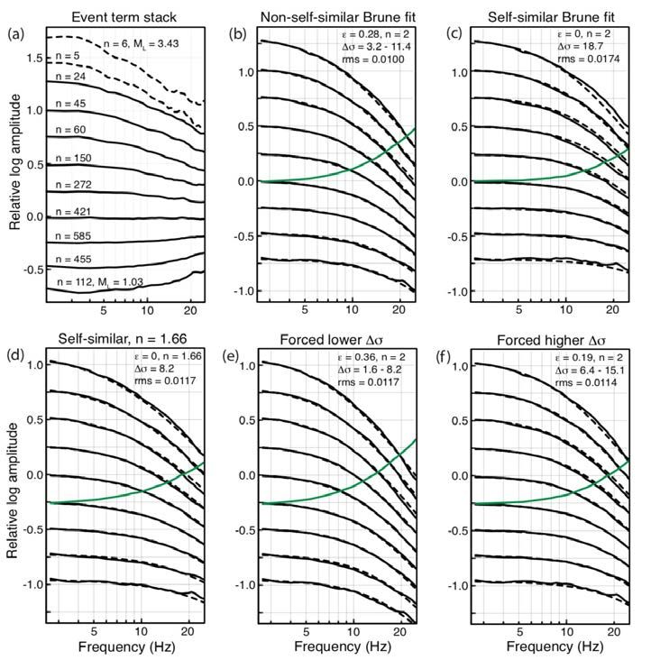
July 5 11:07 Mcat 5.36 ID 38450263                                                         Knudsen and
                                                                                             Ellsworth
  Mw 5.13, stress drop 65 MPa, fc 1.02 Hz

            Measured amplitudes

                                  Best-fitting Brune spectrum
                                                                          Misfit error analysis
        Corrected amplitudes
                                                                          Note covariance between seismic moment
                                                                          and corner frequency

1/26/2023                         Southern California Earthquake Center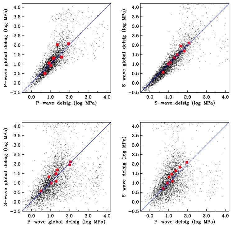
July 5 11:07 Mcat 5.36 ID 38450263                               Knudsen and
                                                                 Ellsworth

 With station terms                  Without station terms

 Mw 5.13                             Mw 5.31
 fc 1.02 Hz                          fc 0.72 Hz              8
 s.d. 65 MPa                         s.d. 42 MPa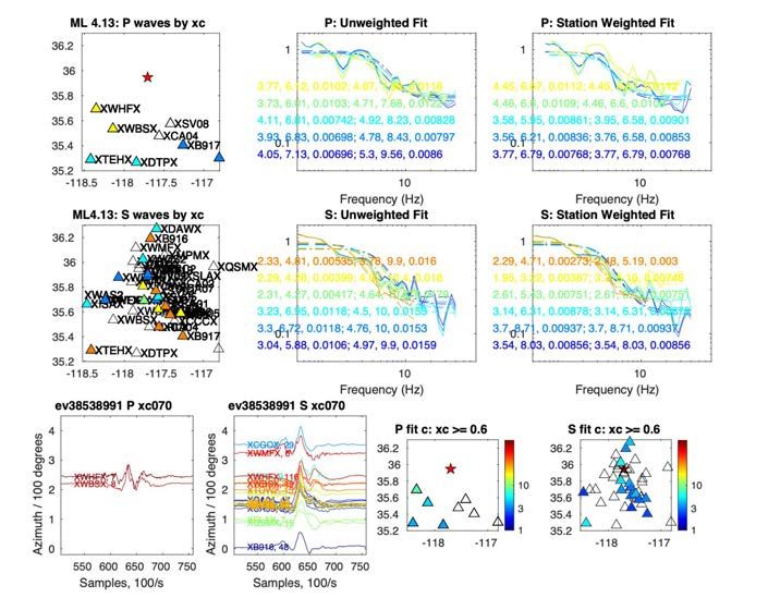
Frequency dependence of attenuation
From Al-Ismail, Ellsworth and Beroza (BSSA, 2023)
Knudsen and
                                           EXTRA SLIDES                                                          Ellsworth

            ID         depth mag         date           time log w0            fc       M0        Mw stress drop

            38445975   2.301 4.04   05-Jul-2019 00:18:01       -3.69           1.65     1.67e15   4.12   8.26
            38451079   7.340 4.09   05-Jul-2019 12:38:30       -3.62           2.44     1.97e15   4.17   31.53
            38471103   7.778 3.30   07-Jul-2019 03:23:26       -4.92           4.62     9.85e13   3.30   10.70
            38483215   7.751 3.13   08-Jul-2019 05:02:10       -5.20           5.15     5.17e13   3.11    7.78
            38450263   7.23 5.36    05-Jul-2019 11:07:53       -1.90           0.72     1.03e17   5.31   42.36
            38538991   2.768 4.13   11-Jul-2019 23:45:18       -3.69           1.99     1.67e15   4.12   14.50
            38489543   2.839 2.5    08-Jul-2019 17:30:03       -5.77           4.38     1.39e13   2.73    1.29
            38496551   10.11 2.57   09-Jul-2019 05:17:45       -5.93          16.28     9.63e12   2.62   45.78

1/26/2023                                       Southern California Earthquake Center
Multi-Method Comparison
Kevin Mayeda, Dino Bindi, Paola Morasca, Jorge Roman-Nieves, Bill
Walter, Doug Dreger, Taka’aki Taira, Chen Ji, Ralph Archuleta
● CCT 2.3CCT vs GIT • 3 common ‘Focus’ events between GIT (Bindi et al., 2021) and CCT spectra are in good agreement. • 2 events (38444103, 38538991) show a pronounced spectral bump near 3-Hz. • Correspondence between GIT and CCT also found in central Italy (Morasca et al., 2022) 9/102022 Southern California Earthquake Center 12
CCT Initial Focus events
38583335 38444103 38538991
• CCT spectra for 3
Focus events.
• Depth dependence in
apparent stress
w/significant outlier
2019-07-06 03:16:32.
9/10/2022
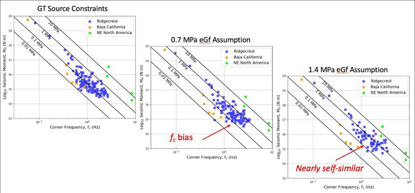
9/102022 Southern California Earthquake Center 13GT Source Constraints
CCT uses reference ‘ground truth’ (GT) spectra
for site term corrections using the coda spectral
ratio method (Mayeda et al., 2007) avoiding
a priori scaling assumptions.
CCT and GIT spectra are in good agreement for an event pair
used in determining GT source spectra used in the CCT
calibration. These spectra along with independent Mw’s for
other events provide the station site corrections.
9/102022 Southern California Earthquake Center 14Comparison of GIT vs Coda CT
● Spectra from GIT and CCT
methods yield similar
radiated energy, Mw and
apparent stress.
● For the larger events, we
find similar results with
ß=3500
those from UCSB (Ji & rho=2700
Archuleta, pers. comm.,
Sept. 2022).
CCT vs GIT: GIT calibration events (~600 solid blue circles) from Bindi et al., (2020;2021) and coda results are
shown as white to deep red circles as a function of the ratio of observed to extrapolated energy (174 events) along
with error bars derived from NLS inversion. Lines of constant apparent stress are shown as reference and similar
to findings from central Italy by Morasca et al., (2022).
9/102022 15Apparent Stress for Larger Events w/UCSB
• We compare results of 25 larger magnitude events
also processed by UCSB (Ji & Archuleta) using three
different methods.
• In general, agreement is good and future study to
understand the outliers is planned.
Figure by Chen Ji and Ralph Archuleta:
GR: using the modified Gutenberg-Richter method (Kanamori, et al., 2020).
Time domain, no local attenuation correction.
F0: frequency approach. Corrects near surface impedance, k_0, crust
attenuation, similar to Boatwright et al. (2003). The
radiation coefficients are assumed to be 0.6 (Boore and Boatwright, 2003).
It is on average 20% larger than GR.
F1: Similar to F0, except we use Caltech moment tensor to estimate
radiation coefficients and only select the measurements with radiation
coefficients larger than 0.25. It is on average 38% larger than GR.
9/102022 Southern California Earthquake Center 168 selected events ID Z Mag date-time CCT fc CCT Mw GIT fc FF fc 38445975 2.3 4.04 ‘05-Jul-2019 00:18:01’ 1.31 4.07 1.02 1.29 38451079 7.3 4.09 ‘05-Jul-2019 12:38:30’ 1.53 4.10 1.54 1.02 38471103 7.7 3.30 ‘07-Jul-2019 03:23:26’ 1.96 3.32 3.43 38483215 7.7 3.13 ‘08-Jul-2019 05:02:10’ 3.41 3.02 4.29 38450263 7.2 5.36 ‘05-Jul-2019 11:07:53’ 0.45 5.37 0.27 0.39 38538991 2.7 4.13 ‘11-Jul-2019 23:45:18’ 1.15 4.13 1.25 0.87 38489543 2.8 2.50 ‘08-Jul-2019 17:30:03’ N/A 38496551 10.1 2.57 ‘09-Jul-2019 05:17:45’ 5.31 2.55 10.18
Comparison with Finite Fault Inversion (Dreger)

              CCT and finite fault estimates of apparent stress and corner frequency for 13 moderate sized
              events (3.27
CCT Mw 2’s and 3’s 38471103 38483215 38496551
CCT Mw 4+

38445975               38451079

38538991               38450263
Summary
●   Varying combinations of GT reference source spectra were tested with no significant
    changes in the final calibration parameters, source spectra, Mw’s and source scaling.
●   Mw’s match those derived from moment-tensor solutions (Validation Mw’s)
    3.4
Source Constraint Affects Site Terms and Scaling
Fixing a handful of Mw 4.0 events to high apparent stress
as ‘reference GT’ biases the scaling.
Using independent GT reference
events from coda ratios we
observe an increase in apparent
stress with moment.
To test the ECS approach, we chose six Mw ~4.0 ‘GT reference events’ to have apparent stress of 0.7 MPa and 1.4 MPa,
which under the Brune source shape assumption is roughly equal to a 3 MPa and 6 MPa Brune stress drop (center and right
figure, respectively). When compared against the calibration that used GT spectral constraints (left), we see a bias at lower
magnitudes and an overall increase in apparent stress over the entire magnitude range. (Note: Only the site terms change.
Path correction and envelope shape remain the same but cannot match original GT ratios in previous slide.)
9/102022 Southern California Earthquake Center 23EXTRA SLIDES ID logMo SElogMo fc SEfc stress_drop_vs_3D SEstdr stress_drop_vs_const 38445975 15.3299270379856 0.048093448591591 1.01800708086084 0.0709773196228018 0.701005826965392 0.153084738877273 0.582907428046382 38451079 15.2838751467793 0.0141603841348427 1.53798101398198 0.0340682640793185 1.40095798764162 0.086164369196776 1.80779101987969 38471103 13.9124399875432 0.0156534898192737 3.43279312034761 0.0965513082003814 0.623354726754051 0.0324365772827538 0.854679006011451 38483215 13.6108637499221 0.0128252383736518 4.29091716382966 0.105832422723926 0.607163883877048 0.0458378593156059 0.833555068929524 38450263 17.6119424143883 0.0883602670144013 0.267276416901024 0.0287987412297874 1.56019827783463 0.592304288984253 2.01950294683978 38538991 15.3238473611207 0.0298362312433606 1.25085386492333 0.0561163992243787 1.22449686483017 0.163947443674182 1.06631922849795 38496551 12.8702041635577 0.0100399566274271 10.1845234583118 0.281673992958635 1.47276926322507 0.30875575880591 2.02509992377904 1/26/2023 Southern California Earthquake Center
NSEC
   Spectral Ratios - Choice of EGF,                                                  P
                                                                                 NSEC/2
          Time Window etc.
  Apply Methods of Abercrombie et al., 2017; 2020
  etc. to Ridgecrest Earthquakes
             Find all Small events within
             2 km epicentral distance
             1.2 and 2.5 M units < main
             (both ranges iteratively decreased IF >>200 EGFs found)
                                                                                     S
             Define time window NSEC = constant * M01/3
             Try 0.5NSEC to get more P waves for close stations

             Try various EGF threshold depending on cross
             correlation and hypocentral depth difference

            Rachel Abercrombie
             Boston University
               rea@bu.edu

1/26/2023                                Southern California Earthquake Center
Rachel
Example EGF Spectral Ratios: Minimum cross correlation =
Abercrombie
[0.5 0.5 0.6 0.7 0.7 0.8 0.9]
38538991 M4.13 Max depth difference to main =
[10 1 10 10 1 10 10]
0.5 NSEC = 3.15 s 1 NSEC = 6.3 s
Caption 1 Caption 2
1/26/2023 Southern California Earthquake CenterRachel
Example EGF Spectral Ratios: Minimum cross correlation =
Abercrombie
[0.5 0.5 0.6 0.7 0.7 0.8 0.9]
38538991 M4.13 Max depth difference to main =
[10 1 10 10 1 10 10]
fc1, fc2, variance (no constraints)
fc1, fc2, variance (limits on fc2)
0.5 NSEC = 3.15 s 1 NSEC = 6.3 s
Caption 1 Caption 2
1/26/2023 Southern California Earthquake CenterLook for consistency in Different Cross correlations? Rachel
Abercrombie
Time Window affects Frequency Range
Comparison of EGF Variation Effects to Other Methods
Fc comparison: NSEC/2
often too short.
Fc: NSEC Time Window
Fc: NSEC/2 Time Window
28Ridgecrest P and S spectral decomposition comparisons
Peter Shearer, Ian Vandevert & Wenyuan Fan
IGPP/SIO/U.C. San DiegoSpectral decomposition
Good for uniform processing
of large data sets.
Variations of this approach
used by Shearer, Allmann,
Chen, Trugman, Oth, and
others.
Completely empirical—a
great advantage but one that
has its limitationsOld approach: Solve for global ECS function and fc model that best fit entire data set
Raw source terms ECS corrected
ECS Dashed
lines show
model
Solve for Δσ model predictions
and Empirical
Correction
Spectrum (ECS)
Source spectra binned by relative momentResults indicate method has too many free parameters!
For Landers cluster, many different
models can fit the data, given tradeoffs
among the model parameters and the
global EGF function.
Thus, we cannot be sure of the absolute
level of stress drop, the high-frequency fall
off rate, or non-self-similar scaling factors.
These issues require independent
constraints on the EGF function.
However, relative differences in stress
drop among events in the same cluster
are well-resolved, when estimated using
the same EGF function.
from Shearer, Abercrombie, Trugman & Wang (2020)New approach: Locally fix small earthquake average corner frequency
Force the Brune corner frequency
(fc) of nearby M 1.5 earthquakes to
30 Hz in estimating the ECS for each
target event.
ECS
This directly determines the ECS at
each location and ensures that any
spectral differences seen in M > 1.5
earthquakes are caused by source
variations rather than inaccurate
path corrections.
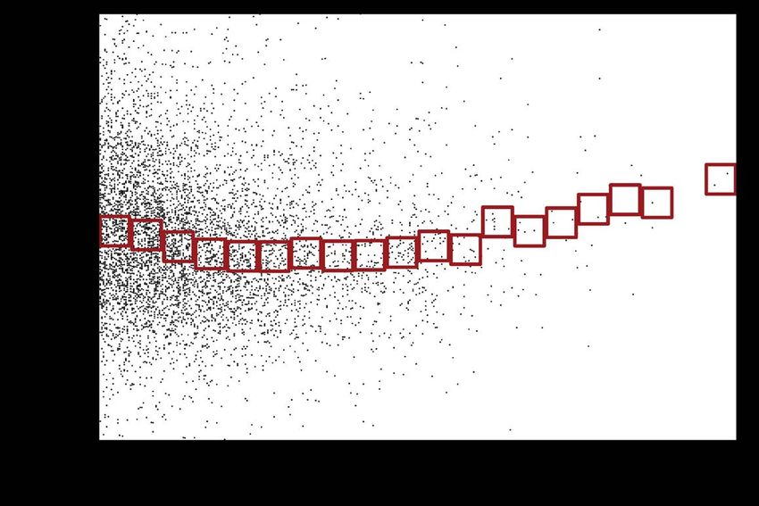
M 1.5 stackOur results for southern California: robust spatial variations
M > 2 only Stress drop estimates for 28,685 M 2 to 4
earthquakes (1996–2019). Each
earthquake has at least 10 M ≤ 1.6
calibration events (assumed to have Brune
fc = 30 Hz) within 5 km in horizontal
distance and 2 km in depth.
These lateral variations in average stress
drop must be real because they are
derived from the relative behavior of M
> 2 quakes with respect to M 1.5 quakes
in each local region, i.e., any
propagation path differences are
removed.
from Shearer, Abercrombie &Trugman (2022)Applications to Ridgecrest test dataset P waves S waves
P waves                    Median stress drop vs. magnitude
                                                  shows increase—is it real?
                                        Increase at M > 3.5 is likely mostly artifact
                                        caused by unresolved low-frequency part of
                                        spectrum and/or HF falloff rate < 2

            Constant for M < 3.5

                      S waves
                                            Somewhat more stable results for
                                            M > 4.5 quakes than P results

               Why the increase here?                    Resolving the low-frequency (< 1 Hz) part of
2x lower Δσ compared to P is related                     the spectrum is key for getting reliable
to moment calibration differences
                                                         results for larger (M > 4) quakes.
Problem: relative moments vs catalog magnitude do not show
expected change in slope as ML changes to Mw for M > 3.5
SCSN P wave analysis Ridgecrest P wave analysis Ridgecrest S wave analysis
Mw in blue
ML in black
from Shearer, Abercrombie &Trugman (2022)Ridgecrest S-wave amplitude decomposition and
comparison to S-wave spectral decomposition
M3.5
Slope = 0.67
Slope = 1.12New method: S-wave amplitude decomposition in the time domain 1. Estimate S-wave arrival 2. Filter entire trace at different frequency bands, measure peak amplitude 3. Assemble observed spectrum 4. Invert to get event terms
Example event term (S-wave displacement)

                     Not very Brune-like!
Empirical correction spectrum (ECS)
ECS
=
observed
spectrum
-
Brune
Brune-like!
solution: force it to be Brune!
(for M1.9-2.1 earthquakes fix a
corner frequency of 14 Hz)Comparison of
spectral
decomposition lower frequency
to amplitude range
decomposition ~0.1 Hzlow frequency
=>
robust momentconsistent spectrum some
shapes differences
spectrum
decomposition and
amplitude
decompositionCorner frequency
estimates from the two
methods correlate with
each other
amplitude
decomposition
and
spectrum
decompositionstress drop estimates from the two
methods correlate with each other (M>3.5)
M3.5-4 M4-4.5 M4.5-5
scale ? scale ? scale ?stress drop estimates from the two
methods show scatters for Mdoes stress drop scale with magnitude?
You can also read


