Keep warm and carry on: Electrification and efficiency meet the "polar vortex" - Synapse ...
←
→
Page content transcription
If your browser does not render page correctly, please read the page content below
Keep warm and carry on:
                      Electrification and efficiency meet the “polar vortex”
                      Asa Hopkins and Kenji Takahashi, Synapse Energy Economics
                    Steven Nadel, American Council for an Energy-Efficient Economy

    ABSTRACT

    Achieving economy-wide greenhouse gas emission reduction targets by mid-century will require
    substantial carbon reductions in space and water heating in buildings as well as in transportation.
    Strategic electrification using efficient heat pump technology coupled with additional energy
    efficiency and an increasingly low-carbon electric supply mix has emerged as the most
    promising combined path for building sector decarbonization. Meanwhile, extreme cold weather
    can stress both the electric and natural gas networks. Electrification will change how these
    stresses play out, impacting the reliability and resource planning for these increasingly
    interlinked energy networks. In this paper, we examine the hypothetical future case of universal
    building decarbonization through electrification when exposed to a “polar vortex” weather event,
    modeled on the event that spread from the Upper Midwest through New England in January
    2019. Using building-level data from the U.S. EIA’s Residential and Commercial Buildings
    Energy Consumption Surveys, we calculate the hourly electric load across four regional markets
    (from MISO to ISO-NE) and estimate the grid impacts of building shell and other efficiency
    improvements, demand response, and the use of hybrid (fossil fuel backup) approaches to
    building electrification. We use this analysis to illustrate how efficiency and load flexibility can
    substantially reduce the future stress on the electric grid and the generation capacity required to
    reliably meet load, as well as the potential for differential regional approaches. From these
    analyses, we draw recommendations for electric and gas system planning and for energy
    efficiency and electrification policies and programs, with the goal of advancing the “strategic” in
    a strategic electrification approach to deep decarbonization.

    Introduction
            Electrification has received increasing attention as a key component of decarbonization,
    alongside increased energy efficiency and increasingly carbon-free electricity (Gowrishankar and
    Levin 2017, NEEP 2017). From state energy plans in the Northeast (Vermont 2016,
    Massachusetts 2018) to new assessments in California (CEC 2019), states and cities are acting to
    displace fossil fuels in buildings with deployment of efficient heap pump technologies. These
    plans recognize that it will be difficult to meet ambitious decarbonization targets, such as net
    zero emissions by 2050, without substantially reducing or eliminating the direct use of fossil
    fuels in buildings. At the national level, electrification plays a major role in the U.S. Mid-Century
    Strategy for Deep Decarbonization (MCS), which is part of the formal U.S. contributions to
    meeting the Paris Agreement (White House 2016).1 The MCS projects electricity’s share of
    energy use in buildings rising from about 50 percent today to about 75 percent by 2050.
            One of the challenges facing building electrification is the changes it will cause on the
    electric grid. Rising electric consumption, driven by electrification of both building and vehicles

    1
     While the U.S. commitment to the Paris Agreement is uncertain, the MCS analysis stands as a useful picture of
    what a largely decarbonized U.S. economy could entail.

©2020 Summer Study on Energy Efficiency in Buildings                                                                 6-96
(plus some industrial electrification), will create the need for an even greater amount of carbon-
free electric supply. NEEP (2017) projects that under a “plausibly optimistic” electrification
pathway in the Northeast, winter electric sales will begin to exceed summer sales in the 2030s. In
the southeast, winter peaks already exceed summer peaks for some utilities (Nadel 2017). With
solar photovoltaic power, which produces best in the summer, as the fastest growing source with
zero marginal emissions this seasonal shift has implications for energy storage, hydropower, and
offshore wind. In heating climates in an electrified world, the coldest periods will create the
largest peaks.
Cold snaps have long created stresses for the energy system. This paper examines one
particular cold event, a “polar vortex” storm that moved from the Upper Midwest through New
England between January 29 and February 1, 2019. On January 30th, the U.S. set a record for
daily total natural gas consumption, and the date had the third-highest residential and commercial
consumption on record. Minnesota gas utility Xcel asked customers to set their thermostats to 63
degrees to reduce strain on the gas system, and a compressor failure in Michigan led Consumers
Energy and the Governor of the state to ask customers to turn down their thermostats, and in the
case of some industrial firms, temporarily stop their production lines. On the electric side,
electric utility DTE asked customers to reduce their electric use, and a nuclear plant in New
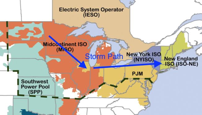
Jersey went offline because its cooling water intake froze over. Figure 1 shows the path of this
event and the electric system context for our analysis.
Figure 1. Map of the area studied in this research. The U.S. area north and east of the
dotted line comprises Census Divisions 1 through 4, while the colored areas show the
regional transmission organizations and the arrow shows the general path of the January
2019 “polar vortex” event.
This paper analyses the hypothetical case in which all the buildings in four Census
Divisions had fully electrified space and water heating when the region experienced the January
2019 polar vortex event. While full electrification is not likely for several decades, examining the
implications now can help us plan for the future. We begin by describing the methodology, using
building-level survey data to estimate the heating loads met by cold-climate heat pumps. We
then present the results of a base case of all air-source heat pumps in today’s buildings, along
with several alternate cases that examine changes in the buildings, heating systems, or occupant
©2020 Summer Study on Energy Efficiency in Buildings 6-97behavior. We conclude with a discussion of the implications of these results for energy planning,
efficiency programs, and the need for innovation.
Methodology
In order to evaluate the potential impact of a polar vortex-like event after complete
electrification of buildings, we used data from the U.S. Energy Information Administration’s
2015 Residential Energy Consumption Survey (RECS) and 2012 Commercial Building Energy
Consumption Survey (CBECS) to estimate the hourly electric load from space and water heating
across the Upper Midwest through the Mid-Atlantic and New England during the 2019 polar
vortex temperature trajectory. RECS and CBECS each provide energy use and building
characteristic microdata for each surveyed building, along with the statistical weight assigned to
each building. RECS and CBECS use statistical techniques to break the full building energy use
into end uses, including space and water heat for each fuel (electricity, natural gas, propane,
heating oil, wood, and district heat). The surveys also provide the heating degree days
experienced by each building.
For each building in Census Divisions 1 through 4,2 we calculated the heat load in BTU
per hour per degree day. We adjusted the reported fuel use to heat delivered by using estimated
heating system efficiency for existing systems. For space heating, we assumed 85% for natural
gas and propane, 75% for heating oil, and 100% for electricity and district heat3. For water
heating, we assumed 92% for electricity, 100% for district heat, and 62% for fossil fuels. When
combined with the temperature trajectory of the polar vortex, this allowed us to calculate the heat
required to maintain temperatures across all buildings in each hour.
We used proxy cities to develop temperature trajectories, which we then assigned to each
building. We used the actual temperatures measured in Minneapolis, Chicago, Columbus,
Philadelphia, Poughkeepsie, NY, and Worcester, MA. All buildings in Census Division 4 (West
North Central) were assigned to Minneapolis weather. All buildings in Census Division 3 (East
North Central) were assigned to Chicago or Columbus weather; we assigned buildings with
heating degree days above the average for the Division (5831 HDD65) to Chicago, and the
remainder to Columbus. We similarly split the Mid-Atlantic division between Poughkeepsie
(colder) and Philadelphia (warmer). New England buildings were assigned Worcester weather.
We assessed the relative impacts of electrification in an average January versus the polar vortex
by also calculating the impact if each city were to experience its average low temperature for
January in the same hour.
To estimate the electric load to meet the heat demand in each building with a cold climate
air source heat pump (ccASHP) system, we used real-world coefficients of performance (COPs)
from Schoenbauer et al. (2017). We used the average of ducted and ductless system
performance, and fit a linear regression for COP versus outdoor temperature, to reflect real-
world system behavior. We also fixed the COP below -13 degrees Fahrenheit to 1.0 to reflect
electric resistance backup heat when it is too cold for today’s air source heat pump systems to
operate. Our analysis converts all buildings to cold climate heat pumps, including buildings with
2
Census Division 1 contains the six New England states. Division 2 (Mid-Atlantic) is New York, Pennsylvania,
Delaware, Maryland, and Washington, DC. Division 3 (East North Central) is Ohio, Indiana, Illinois, Michigan, and
Wisconsin. Division 4 (West North Central) is Minnesota, Iowa, Missouri, the Dakotas, Nebraska, and Kansas.
3
The surveys appear to use the amount of heat delivered to the building by a district heating system, so the
adjustment for efficiency happens upstream of our analysis.
©2020 Summer Study on Energy Efficiency in Buildings 6-98electric resistance heat. Figure 2 shows the hourly temperatures for each city, along with the
estimated ccASHP COPs during each hour.
40
30
20
Philadelphia
Temparature (deg. F)
10 Columbus
Poughkeepsie
January 30 January 31 Worcester
0 Chicago
10 AM
1 PM
4 PM
7 PM
10 PM
10 AM
1 PM
4 PM
7 PM
10 PM
1 AM
4 AM
7 AM
1 AM
4 AM
7 AM
Minneapolis
-10
-20
-30
-40
4.0
3.5
3.0
Coefficient of Performance
Philadelphia
2.5 Columbus
Poughkeepsie
Worcester
2.0 Chicago
Minneapolis
1.5
1.0
0.5
January 30 January 31
0.0
1 AM
4 AM
7 AM
10 AM
1 PM
4 PM
7 PM
10 PM
1 AM
4 AM
7 AM
10 AM
1 PM
4 PM
7 PM
10 PM
Figure 2. Hourly temperatures (top) and modeled coefficients of performance
(COPs) (bottom) for January 30-31, 2019. Source: Synapse analysis;
temperatures from NOAA
We also evaluated other potential heat pumps. For ground-source systems, we assumed a
COP of 3.5 regardless of outdoor temperature.4 We also modeled a higher average performance
for ccASHPs, reflecting future innovation. The high-performance ccASHP system was modeled
with an average COP 0.4 points higher than our baseline case, with heat pump operation
sustained down to -23 degrees, rather than -13. We further modeled an air source system that
retains a combustion backup system (referred to as a dual-fuel system) that transitions to use the
combustion heat source below some (adjustable) temperature. For buildings currently heated
with electric resistance, we assumed that source would remain as the backup heat (rather than
assume the installation of a combustion system).
RECS and CBECS also estimate the annual water heating energy use in each building.
We did not assume any dependence of water heating energy use on outdoor temperature,
4
COPs of GSHP systems on the market today extend as high as 5.7, however the bulk of highly efficient GSHP
have a COP between 3.6 and 4.5, without including the energy use for water pumping (Energy Star 2020).
©2020 Summer Study on Energy Efficiency in Buildings 6-99although we did account for heat pump water heaters creating additional heat load within a
building that must be made up by the space heating system. We used average hourly water
heating load profiles for residential and commercial buildings from EPRI (2020). We did not
include any electric load from other potentially electrifiable end uses such as cooking or laundry,
nor electric vehicle loads. In the context of a polar vortex, it is reasonable to assume that some
amount of voluntary reduction in driving and EV charging would be achievable. During the 2019
polar vortex, many employees were asked to stay at home and authorities encouraged people to
stay off the roads.
To provide a baseline to which newly electrified loads would be added, we calculated the
sum of the actual hourly loads in four regional transmission organizations during the polar vortex
event: the Midcontinent, New York, and New England Independent System Operators (MISO,
NYISO, and ISO-NE), and PJM. These areas cover, but extend beyond, the areas of the four
Census Divisions in our analysis, and also beyond the areas sharply affected by the 2019 polar
vortex event. If loads in the areas covered by MISO and PJM but outside our analysis area were
also increased due to electrification, the overall loads would be higher than we present. However,
as we will discuss below, these loads are likely small compared with the loads from the
examined areas that were both populous and very cold. When adding newly electrified loads to
the actual wholesale generation from 2019, we increase the end-use loads by 10% to account for
increased marginal line losses on the transmission and distribution (T&D) system. While T&D
losses average about 5% in the US over the year (Vidangos et al. 2019), marginal losses at peak
times are generally much higher (Lazar and Baldwin 2011).
Demand-side measures could avoid the need for additional generation, transmission, and
distribution capacity created by electrification. To estimate the benefits of these demand-side
measures, we used avoided cost values of $98/kW-year for avoided generation capacity (based
on Newell et al. (2018)) and $66/kW-year for avoided T&D capacity (the average value across
the country identified in Mendota (2014)). This results in a combined levelized value of
$164/kW-year.
Results with Cold Climate Air Source Heat Pumps
Electrification load under typical winter weather
We examined the load if the study area were to experience its average winter low
temperature simultaneously, in order to separate the load due to electrification from the load due
to a polar vortex event in particular. (The polar vortex event had low temperatures that were
between 20 and 41 degrees lower than the typical low across the study area.) These results
indicate the additional load that the grid might need to meet in typical winters under a fully
electrified future. Table 1 shows the load by assigned city and Census Division. By way of
comparison, the (noncoincident) 2018 summer peak across the four RTOs was approximately
330 GW, about 65 GW lower than the electrified peak under the average January low
temperature.5 Thus, the region would require some additional capacity in order to be able to
support a fully electrified future, even without a polar vortex (assuming no change in underlying
energy efficiency).
5
Table 1 shows an additional 116 GW of normal winter cold load. Of this, about 51 GW can be supplied by the
difference between the 330 GW 2018 summer peak and the 279 GW 2018 winter peak, leaving a need for 65 GW of
new capacity.
©2020 Summer Study on Energy Efficiency in Buildings 6-100Table 1. Additional electrification load during typical winter cold weather, by weather-
proxy city and Census Division.
Weather-Proxy Normal Winter Census Division Normal Winter
City Cold Load (GW) Cold Load (GW)
Minneapolis 23 West North Central 23
Chicago 23
East North Central 42
Columbus 19
Philadelphia 21
Mid-Atlantic 35
Poughkeepsie 14
Worcester 16 New England 16
Total 116
Load during the 2019 Polar Vortex event
The coincident coldest temperatures from 2019 polar vortex event peaked across the full
region in the morning of January 31. This corresponded closely with the morning peak load
experienced across the RTOs. The total system peak during this hour would have been 690 GW,
an increase of a factor of 2.5 from the load experienced in this hour in 2019. Relative to an
electrified future with typical cold January weather, the load would be about 70 percent higher.
Figure 3 shows the hourly loads, broken out by additional residential and commercial, as well as
the 2019 actual. Space heating is responsible for all but 21 GW of the increase in load in the peak
hour. Loads would have fallen quickly after 8 AM on the 31st as the air rapidly warmed across
the region. All of these figures are for actual loads and do not include a reserve margin.
800
700
600
Load across 4 RTOs (GW)
500
400
Residential
300 Commercial
2019 load
200
100
January 30 January 31
-
1:00:00 AM
4:00:00 AM
7:00:00 AM
10:00:00 AM
1:00:00 PM
4:00:00 PM
7:00:00 PM
10:00:00 PM
1:00:00 AM
4:00:00 AM
7:00:00 AM
10:00:00 AM
1:00:00 PM
4:00:00 PM
7:00:00 PM
10:00:00 PM
Figure 3. Hourly modeled load during the polar vortex period, showing the actual
2019 load (blue) and the incremental electrification loads from space and water
heating for ccASHP-heated residential (grey) and commercial (orange) buildings.
Alternate Cases
The remarkable increase in peak loads estimated in the previous section inspires an
examination of what the impact of potential alternate paths would be for buildings and the grid.
This section briefly summarizes the results in six alternate cases.
©2020 Summer Study on Energy Efficiency in Buildings 6-101Building shell improvements and other home energy efficiency improvements
The building stock across the study area is relatively old, and many buildings could
benefit from substantial air sealing and insulation retrofits. In addition, over the time between
now and when all buildings could be electrified, new construction will improve the average
building shell performance. In addition, better lighting and appliances would reduce electric
loads. To estimate the impact of universal improvement in building shells plus other efficiency
improvements, we modeled a reduction in heat and other loads of 25 percent across all buildings,
retaining the base case ccASHP systems. A Home Performance with Energy Star retrofit
typically reduces energy use 25% (Dunn 2019). Kwatra and Essig (2014) identify similar savings
from whole building commercial retrofits. Deep retrofits can save more (e.g., 50% or more in
site heating load reduction), but we assumed a more typical whole building retrofit as the average
across all buildings since not all buildings will be weatherized. This lowers the peak of the
combined electric load to 502 GW, a reduction of 189 GW from the base case.
If supplying generation capacity and a transmission and distribution (T&D) system to
meet an incremental kW of peak load has a cost of $164/kW-yr, avoiding this cost via energy
efficiency would provide a system value of $30.9 billion per year, or a present value of $460
billion over 20 years (at a 3% real discount rate). Allocated to residential and commercial
buildings on an electric heating load basis, this would represent a value of $6,200 per household
and $4.80 per square foot of commercial space. This value does not include the value of energy
savings accruing over the year, nor does it include summer savings from reduced air
conditioning loads.
Demand response
In the polar vortex of 2019, gas and electric utilities asked customers to set back their
thermostats to reduce demand on the energy system. With smaller temperature differentials
between inside and outside, heat losses are reduced and energy demand falls. This type of
voluntary demand response could be amplified by smart thermostats or other automated systems.
To evaluate the potential for peak electric savings during an electrified polar vortex, we modeled
a case in which indoor temperatures were reduced by 5 degrees throughout the study period. This
lowers the peak of the combined electric load to 665 GW, a reduction of 26 GW from the base
case.
Higher-performance air-source heat pumps
Technological innovation could improve the performance of air-source heat pumps along
two important dimensions: extending heat pump operation to lower temperatures, and higher
COPs at all temperatures. We modeled a case in which the relationship between COP and
temperature is shifted ten degrees: heat pump operation continues down to -23 degrees F, and
COPs at each temperature are the same as what they would have been ten degrees warmer. For
example, the high-performance COP at zero degrees F, 2.51, is what the base case ccASHP
delivers at 10 degrees.6 Extending heat pump operation to lower temperatures allows heat pump
operation throughout the polar vortex event except in the West North Central (with Minneapolis
6
This is equivalent to increasing the COP by about 0.4 points or the heating season performance factor (HSPF) of
the heat pump by 1.36 points.
©2020 Summer Study on Energy Efficiency in Buildings 6-102weather). With improved ccASHPs, the hourly peak electric demand peaks at 600 GW, a
reduction of 90 GW from the base-case of ccASHP performance.
Ground-source heat pumps
Ground-source heat pumps (GSHPs) generally have a high COP (we assumed an average
of 3.5) and the COP is independent of the air temperature. The heat load is still linearly
dependent on outdoor temperature, but incremental loads from electrification are much closer to
the “typical weather” case than the base case ccASHP. The hourly electric demand peaks at 435
GW at 8 AM on January 31st. This represents a reduction in peak demand of 256 GW vs. the
ccASHP case.
GSHP savings relative to ccASHPs are concentrated in the Midwest (Census Divisions 3
and 4), where the polar vortex took temperatures below -13 and electric resistance backup heat is
required with today’s ccASHPs. Net peak savings from GSHPs in the West North Central are 79
percent of the ccASHP incremental load, while they are only 49 percent in New England.7 We
also examined a case where all space heating electrification happens via GSHPs in the Midwest,
and via ccASHPs in the Mid-Atlantic and New England. In this case, the peak load is 502 GW –
a reduction of 188 GW from the all-air-source case, and an increase of 68 GW over the all-
ground-source case.
Dual-fuel heat pumps
Another approach to mitigating electric peak load is to switch to combustion fuel below a
transition temperature. Some utilities, such as Hydro Québec, which have substantial electric
heating, use dual-fuel systems as a kind of demand response to mitigate winter peak loads
(Hydro Québec 2020). In the polar vortex context, many locations would be below the transition
temperature throughout the event. With dual-fuel heat pumps, the additional electric load is
relatively small during much of the vortex due to use of backup fuel, but peaks emerge at the end
of the study period, as it warms up enough for heat pumps to take over the load. We examined
the tradeoff between transition temperature and peak electric load; the results are shown in
Figure 4. When the transition temperature is below -6 degrees, the only use of dual-fuel systems
is in the Midwest, but peak reductions remain substantial (more than 180 GW below the ccASHP
base case) because temperatures in that region were so cold.
7
The ratio is not simply a result of the COPs of the different technologies at cold temperatures, due to the assumed
conversion of electric resistance-heated homes to heat pumps.
©2020 Summer Study on Energy Efficiency in Buildings 6-103400
350
Max. New Space Heating Load (GW)
300
250
200
150
100
50
-
-25 -20 -15 -10 -5 0 5 10 15 20
Transition Temperature to Combustion Backup Heat (deg. F)
Figure 4. As the transition temperature between electric and
combustion systems is lowered, the maximum new electric heating load
increases.
Combined efficiency improvements, demand response, and ground-source or dual-fuel heat
pumps
With better building shells and other efficiency improvements, higher-efficiency heat
pumps, responsive customers willing to reduce indoor temperatures during cold snaps, and use of
ground-source or dual-fuel heat pumps, the total impact of electrification can be substantially
reduced. We illustrate this with cases that combine 25 percent efficiency improvements, a 5-
degree setback, and use of either dual-fuel heat pumps (with a transition temperature of zero
degrees) or GSHPs in the colder parts of the Midwest. (We retain ccASHPs in the warmer parts
of the East North Central division as well as all of Mid-Atlantic and New England, where the
coldest temperatures are not reached.) The resulting load trajectories are shown in Figure 5,
alongside a dotted line showing the base-case ccASHP loads.
The GSHP case shows loads that are 260 GW (38 percent) below the ccASHP-only base
case, while the dual fuel case is even lower at the coldest time, 290 GW (42 percent) below the
base case peak. These cases could have a present value of $634 billion and $707 billion,
respectively, in generation capacity and T&D savings over 20 years. Allocated to residential and
commercial buildings on an electric heating load basis, this would represent a value of:
• $2,700 per household and $2.00 per square foot of commercial space in the Mid-
Atlantic and New England, from efficiency and demand response
• $13,300 per house and $10.30 per square foot of commercial space in the two
Midwestern regions in the GSHP, EE and DR case, and
• $15,100 per house and $11.70 per square foot of commercial space in the two
Midwestern regions in the dual-fuel HP, EE and DR case.
Again, these values do not include the value of energy savings, nor do they include summer
savings from reduced air conditioning loads.
©2020 Summer Study on Energy Efficiency in Buildings 6-104800
700
600
Load Across 4 RTOs (GW)
500
ccASHP Base Load
400
EE + DR + GSHP
300 EE + DR + Dual Fuel
2019 load
200
100
January 30 January 31
-
1 AM
4 AM
7 AM
10 AM
1 PM
4 PM
7 PM
10 PM
1 AM
4 AM
7 AM
10 AM
1 PM
4 PM
7 PM
10 PM
Figure 5. Modeled hourly load during the polar vortex with additional energy
efficiency throughout each building, 5-degree thermostat setback, and either GSHP
or dual-fuel HPs in the West North Central division and the colder locations in East
North Central.
Discussion
Winter demand peaks, especially during rare but deep cold events, would have
profoundly different effects on the electric grid after mass electrification than they do today.
Rarely used generation or storage assets would be required to meet rare peaks that are
substantially higher than the loads experienced during typical winter weather, while transmission
and distribution systems would similarly be required to be built to handle these rare but very high
loads. The difference between summer 2018 peak demand and winter 2019 peak demand
indicates there would be about 50 GW of generation, transmission, and distribution capacity
available in the region to help serve increased winter peak demand if the transition were to occur
overnight. Above that level, the overall region would become winter peaking.
Energy efficiency, in the form of better building shells or higher-performing electric
heating equipment, could have a substantial positive effect on the capacity needs of the electric
grid, and customers willing to reduce indoor temperatures on rare occasions could similarly save
billions of dollars in system costs.
The impacts of each of the alternatives we examined are summarized in Table 2. As can
be seen, the largest impacts are from energy efficiency, ground-source heat pumps, and dual-fuel
heat pumps. Higher-performing ASHPs do not deliver the savings seen from GSHPs or dual fuel
systems, but could be less expensive than either drilling wells for GSHPs or maintaining the full
gas heating infrastructure to use on an occasional basis, especially if combined with additional
energy efficiency. Demand response has less impact than other methods because indoor-outdoor
temperature differentials remain very large compared to reasonable thermostat setbacks at these
extreme temperatures. These measures can be combined – when we combine efficiency and
demand response with ground-source heat pumps or dual-fuel heat pumps where the air
temperatures are lowest, the peak load after full space and water heating electrification for the
residential and commercial sectors declines from 690 GW to 331 or 361 GW, a reduction of
©2020 Summer Study on Energy Efficiency in Buildings 6-105about a factor of two. Winter peak loads in the combined case are only a little higher than current
summer peak loads across the region.8
Table 2. Summary results of the cases modeled, including (in the final column) the actual peak load in the hour
ending 8AM on January 31, 2019.
New Res. Peak New Com. Peak Total New Peak Total Load at
Load (GW) Load (GW) Load (GW) Peak (GW)
ccASHPs 269 138 411 690
ccASHPs w/ 25% EE 206 107 313 502
ccASHPs w/ DR setback 252 133 385 665
High-perf ccASHP 213 108 321 600
GSHP 100 55 155 435
Dual Fuel HP 39 50 90 369
EE + DR + GSHP 91 39 130 361
EE + DR + Dual Fuel 72 28 100 331
These results clearly show the value of energy efficiency measures and innovation.
Innovation will be critical for continued improvements in heat pumps and in techniques to
weatherize homes and buildings, and to convince building owners to make the necessary
improvements. Taken together, efficiency and innovation dramatically reduce the peak impacts
of electrification. Incentives and inducements will be needed for such innovation to be realized.
Even with efficiency and innovation, the impacts of full electrification are still
substantial. Our analysis indicates a need in our combined case, after subtracting the current
difference between summer and winter peaks, for about 35 to 70 GW of capacity (including a 10
percent reserve margin), an increase of about 10 to 20 percent relative to today. Additional
generation will be needed, as will T&D improvements to buttress the grid. Long-term storage
(e.g. enough to handle a multi-day polar vortex) would also be useful to reduce the needed
generation, but this storage will also need a value proposition during normal weather; such
storage is another area for needed innovation. And further work is needed to figure out the best
generation resources for cold winter days. For example, during the vortex, skies were generally
clear and therefore solar energy could be generated, but only during limited daylight hours. Wind
performed well, but some resources were forced offline by cold temperatures. Hydropower in the
region is available but limited. The remaining power could come from nuclear or peaking plants,
the latter fueled with fossil or synthetic natural gas or perhaps hydrogen.
Full electrification will not happen overnight – in all likelihood it will be at least 2050
before full electrification is possible. Thus, the impacts on the grid will be gradual, and there will
be time to plan for needed grid improvements. If the transition modeled here were to take place
over 30 years, the rate of peak increase would not be substantially different from that
experienced in much of the latter half of the 20th Century. Still, grid- and energy-planners should
start considering increased building electrification as they develop long-term scenarios. Our
analysis is very high level. Additional more detailed analysis is needed, particularly at the power
pool level where most resource planning takes place.
8
Increased T&D capacity may not be necessary to meet the winter peak loads in the combined case even if the load
is higher that today’s summer loads (in MW terms) because winter ratings for the existing T&D system components
are likely to be higher than these components’ summer ratings.
©2020 Summer Study on Energy Efficiency in Buildings 6-106In addition to grid impacts, the scenarios we provide have large impacts on the natural
gas system. Electrification, including dual-fuel heat pumps, means much lower sales for gas
utilities and therefore higher customer prices for pipeline gas because fixed costs of gas
infrastructure will need to be spread across reduced sales. In warm regions, phasing out gas
infrastructure may make sense, but in the upper Midwest, given the very low temperatures
sometimes reached, this will be unlikely. And if gas infrastructure is reduced, ways to cushion
the cost impacts to gas companies and ratepayers will need to be explored. Competition between
ground-source and dual-fuel heat pumps in these very cold regions will be shaped by innovation,
policy, and infrastructure choices.
Overall, electrification will likely be a critical strategy for meeting long-term
decarbonization goals. But full electrification will have large impacts on the electric grids and
gas infrastructure. Our analysis illustrates these potential impacts, but also how they can be
reduced through use of efficiency, demand response, and innovation.
References
California Energy Commission (CEC). 2019. Building Decarbonization Assessment Project
Scope. Docket Number 19-DECARB-01.
https://efiling.energy.ca.gov/Lists/DocketLog.aspx?docketnumber=19-DECARB-01
Dunn, S. 2019. “Home Performance with Energy Star.” Presentation at BTO Peer Review, April
17. https://www.energy.gov/sites/prod/files/2019/05/f62/bto-peer-2019-rbi-partnerships-
1.pdf.
Electric Power Research Institute (EPRI). 2020. “Load Shape Library 7.0; End-Use Load
Shapes”. Accessed at https://loadshape.epri.com/enduse in March, 2020.
Energy Star. 2020. “ENERGY STAR Most Efficient 2020 — Geothermal Heat Pumps.”
Accessed at
https://www.energystar.gov/products/energy_star_most_efficient_2020/geothermal_heat_pu
mps in March, 2020
Gowrishankar, V. and A. Levin. 2017. America’s Clean Energy Frontier: The Pathway to a
Safer Climate Future. New York, NY: Natural Resources Defense Council.
www.nrdc.org/resources/americas-clean-energy-frontier-pathway-safer-climate-future .
Hydro Québec. 2020. “Rate DT – Dual Energy.” Access at
http://www.hydroquebec.com/residential/customer-space/rates/rate-dt.html in March, 2020.
Kwatra, S. and C. Essig. 2014. The Promise and Potential of Commercial Building
Comprehensive Retrofit Programs. Washington, DC: ACEEE.
https://www.aceee.org/research-report/a1402.
Lazar, J. and X. Baldwin. 2011. Valuing the Contribution of Energy Efficiency to Avoided
Marginal Line Losses and Reserve Requirements. Montpelier, VT: RAP.
https://www.raponline.org/wp-content/uploads/2016/05/rap-lazar-eeandlinelosses-2011-08-
17.pdf.
©2020 Summer Study on Energy Efficiency in Buildings 6-107Massachusetts Department of Energy Resources. 2018. Massachusetts Comprehensive Energy
Plan. Boston, MA: DOER. https://www.mass.gov/service-details/massachusetts-
comprehensive-energy-plan-cep
Mendota Group, The. 2014. Benchmarking Transmission and Distribution Costs Avoided by
Energy Efficiency Investments. https://mendotagroup.com/wp-
content/uploads/2018/01/PSCo-Benchmarking-Avoided-TD-Costs.pdf
Nadel. 2017. Electricity consumption and peak demand scenarios for the Southeastern United
States. Washington, DC: ACEEE. www.aceee.org/research-report/u1704
Newell, S., J. M. Hagerty, J. Pfeifenberg, B. Zhou, E. Shorin, P. Fitz, S. Gang, P. Daou, and J,.
Wroble. 2018. PJM Cost of New Entry; Combustion Turbines and Combined-Cycle Plants
with June 1, 2022 Online Date. Cambridge, MA: The Brattle Group.
https://www.pjm.com/~/media/committees-groups/committees/mic/20180425-
special/20180425-pjm-2018-cost-of-new-entry-study.ashx.
Northeast Energy Efficiency Partnerships (NEEP). 2017. Northeastern Regional Assessment of
Strategic Electrification.
https://neep.org/sites/default/files/Strategic%20Electrification%20Regional%20Assessment.p
df.
Schoenbauer, B., N. Kessler, and M. Kushler. 2017. Cold Climate Air Source Heat Pump.
Conservation Applied Research and Development (CARD) FINAL Report, Nov. 1, 2017.
https://www.mncee.org/MNCEE/media/PDFs/86417-Cold-Climate-Air-Source-Heat-Pump-
(CARD-Final-Report-2018).pdf
Vermont Department of Public Service (Vermont). 2016. 2016 Vermont Comprehensive Energy
Plan. Montpelier, VT: DPS. https://publicservice.vermont.gov/publications-
resources/publications/energy_plan/2015_plan
Vidangos, N., M. Scerbo, S. Nadel, L. Ungar and E. Cooper. 2019. Energy Efficiency Impact
Report. Washington, DC: Alliance to Save Energy, American Council for an Energy-
Efficient Economy and Business Council for Sustainable Energy.
https://energyefficiencyimpact.org/.
White House, The. 2016. United States Mid-Century Strategy for Deep Decarbonization.
Washington, DC: The White House. https://unfccc.int/files/focus/long-
term_strategies/application/pdf/mid_century_strategy_report-final_red.pdf.
©2020 Summer Study on Energy Efficiency in Buildings 6-108You can also read