Why do we need simulation? Dynamic complexity
←
→
Page content transcription
If your browser does not render page correctly, please read the page content below

Computer simulation:
06                                                                      Helping us not to
                                                                        cheat at solitaire
                        Construction Dynamics Solutions LLC – On Disruption and Delay

Why do we need simulation? Dynamic complexity
When trying to understand and/or manage disruption and delay on complex projects, we need computer
simulation because it is the only way in which we can deal with the “dynamic complexity” inherent to these
projects.
Normally, when we think about “complexity” we imagine situations in which we have to deal with large
quantities of data, and/or where we have to consider numerous decision factors simultaneously. Dealing with
complexity is clearly not easy, but over the last few decades (and especially following the invention of the
modern computer), we have developed ever more sophisticated tools to help us in this regard – in the field of
project management, the best example of this are probably project planning and control tools based on the
Critical Path Method (‘CPM’), and/or on Building Information Modelling (‘BIM’.)
And yet, neither our brains nor the tools mentioned above have so far helped us to deal effectively with
disruption (and therefore, also often not with delay, either.) Why has this been the case? Because projects are
not simply complex, they are dynamically complex.

         Figure 1: A dynamic causal framework for delay and disruption on complex construction projects.

In a previous article in this series, we described the causal framework that explains how complex projects are
disrupted, how disruption spreads, and how it interacts with delays (see Figure 1.) 1 This framework consists of
many different factors, all of them impacting project performance as well as each other – but there is more to
it than that: Project dynamics are driven by feedback, they are non-linear, and responses to causes can

1
    See our previous article “02 A Causal Framework for Disruption and Delay: Loopy, not Straight”. All the articles in this
    series can be downloaded from our website at www.constructiondynamics.global/publications.

© Construction Dynamics Solutions LLC 2021                                                                             1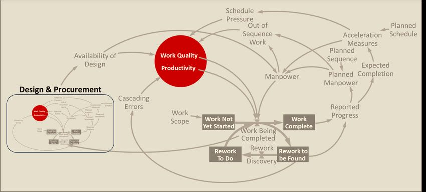
Computer Simulation: How Not to Cheat Ourselves at Solitaire

manifest themselves after significant delays. These are the three characteristics that make the complexity
inherent to project performance dynamic:

       •    Feedback. When a causal chain forms a circle, causation never stops: the past influences the present,
            and the present influences the future. In dynamic systems, capturing how causation flows through
            time is critical in order to understand past performance, or to predict the future.

                                        Figure 2: Disruption and delay feed on each other.

            A typical example of feedback is the interaction between delay and disruption: Once a project is
            delayed, managers typically take mitigation actions, which usually lead to some disruption2… which
            again slows down the project… and so new mitigation measures are implemented… and so on.

       •    Non-linearity. Systems with feedback are inherently non-linear, and most management decisions lead
            to unanticipated side-effects.3 But also: Projects are subject to many types of limits, so that (for
            example), doubling resources never cuts the duration of the project in half. Or: The cumulative
            disruptive impact of a series of small changes gets inordinately stronger as more changes pile on.

       •    Delayed responses: Finally, in dynamic systems the consequences of a decision may not manifest
            themselves for some time, thus (a) driving decision-makers to overreact, or (b) lulling them into
            deceptive complacency. A good example of this is rework: A decision to rush work to meet a milestone
            may look to be correct if the milestone is reached… until a raft of work defects are detected weeks (or
            months) later, considerably slowing down the project overall.

These three characteristics are a reality of projects, so we need to be able to account for them properly in any
analysis that we do. So, the question is: How can we do this?

The need for simulation
When human beings try to deal with complex, dynamic systems without the support of proper analytical tools,
the decisions made are often wrong, ineffectual, or even counterproductive 4. Thankfully, there is one
analytical tool that can deal with dynamic complexity: Simulation.

2
    Ibid.
3
    Dealing with non-linearity is especially complicated because human brains are so poorly equipped to handle it. For more
    on this topic, please see the appendix to this article.
4
    See Forrester, Jay W., “Principles of Systems”, p. 3-2, Productivity Press (1990.)

© Construction Dynamics Solutions LLC 2021                                                                            2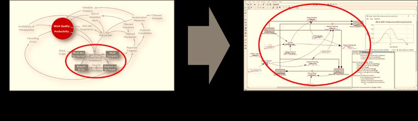
Computer Simulation: How Not to Cheat Ourselves at Solitaire

Why simulation? Because translating a causal framework as the one shown in Figure 1 into mathematics
requires hundreds of equations – and their “dynamic” characteristics will require that many of these will be
differential equations, dealing with feedback (recursiveness), delays and on-linearity. It is completely
impossible to solve such a large system of simultaneous differential equations directly, so simulation becomes
the only viable option.
(Added bonus: You don’t need to know anything about systems of differential equations to run or to
understand dynamic simulation models – you’ll see!)

How does simulation work? A simple example
To explain in detail how a dynamic simulation model works, we will focus on a much-simplified version of the
delay and disruption causal framework shown in Figure 1, and describe mathematically its performance over
time. However, before we can do this, we need to quickly discuss how computers deal with “time”.

The concept of the “time step”
To our human mind “time” flows continuously, and we can divide it into as many infinitesimal slices as we
want; however, computers cannot handle the abstract concept of “infinitesimal”, and they need to break
down time into discrete “steps”5. Thus, to simulate the evolution of a project, computers will:
       a) Take the project’s conditions “now”;
       b) Based on these, they will extrapolate the project’s conditions one small step into the future;
       c) Then, this future time becomes the new “now”, and the process repeats itself… one time step after
          another, until the end of the period being simulated.

    Figure 3: Simulation models extrapolate from current conditions, one small step into the future at a time.

To help understand this concept, let us imagine a car going down a highway. At a constant speed, we could
predict its future location at any point in the future, just by multiplying time by speed. But, what if its speed
was variable? One solution would be to chop down time into very small steps, so small that speed could be
considered to be “practically” constant within each step – and we know how to calculate position when speed
it constant! This, in essence, is what simulation does.
How small should the time step be? Well, it depends on the speed at which dynamics unfold in the system: If
we want to simulate the speed and position of a celestial body, using a time step of one day may produce
perfectly accurate results – but if we were analysing a rocket launch instead, a time step as small as a second
would probably still be way too long. On complex construction and engineering projects, dynamics usually
take weeks or months to fully unfold, so a time step of a few days is usually adequate.

5
    This, by the way, is how Newton and Leibniz developed Calculus.

© Construction Dynamics Solutions LLC 2021                                                                  3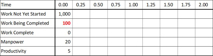
Computer Simulation: How Not to Cheat Ourselves at Solitaire

Simulating a “simple” project
As stated earlier, we will simulate just a small part of the causal framework for disruption and delay, to keep
the example simple. The fragment that we have chosen describes the following (see Figure 4):
    a) At the beginning of the Project no work has been started yet, so the whole scope of work is yet “Work
       Not Yet Started”.
    b) Then, as manpower is applied, work is accomplished (“Work Being Completed”)…
    c) … and thus, over time, more and more work can be considered “done” (“Work Complete”.)

      Figure 4: Our example will focus on a small section of the delay and disruption causal framework.

Note that in this simplified framework (a) there is no rework, (b) productivity is assumed to be constant, and
(c) so is manpower. While this may not be a very realistic description of how projects work (too simple), it will
still serve as a perfect example to demonstrate how simulation works – and its simplicity will help us to keep
the math manageable.

Describing our project mathematically
Our first step will be to describe our “simple” project in mathematical terms – after all, this is the only language
that computers will understand. Figure 5 shows what these equations would be:

 Figure 5: Mathematical equations describing the dynamics in the section of the framework being analysed.

© Construction Dynamics Solutions LLC 2021                                                                     4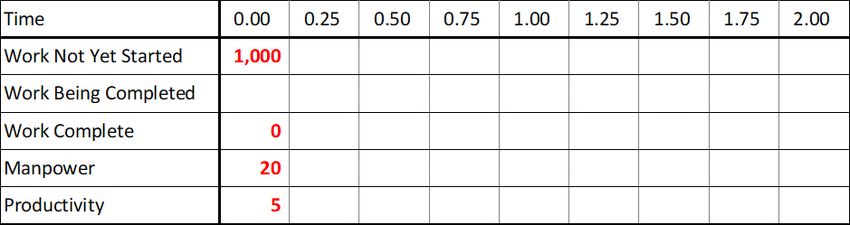
Computer Simulation: How Not to Cheat Ourselves at Solitaire

These equations may look like a mouthful, but they are simpler than they may appear at first glance. To better
understand them, we will look at them step by step.:
      a) First, there are certain variables that have a constant value throughout the project, and which can
         thus be described by a number (see Figure 5.) In our case, manpower will be held at 20 people, we
         will assume that these people will achieve a constant productivity of 5 activities per person per month,
         and the total scope of work to be done will be 1,000 activities:

                     Figure 6: Some project variables have constant values throughout the project.

      b) Then, some of the variables in the framework are “stocks”, accumulations over time (represented by
         grey boxes in Figure 4): the amount of “Work Complete”, and the amount of “Work Yet to Be Started”
         (work done is subtracted from this variable – and subtraction is nothing but a “negative”
         accumulation.) The equations for these stocks are simple: their values for the next time step (at time
         “t+dt”) are equal to their values now (at time “t”), plus or minus the rate at which they are changing
         now (a separately defined variable) times the length of the time step (“dt”).

                       Figure 7: Some variables represent “stocks”, accumulations over time.

           So, for example: if (i) we now had a stock of 200 completed activities, and (ii) we were completing 40
           additional activities per month, and (iii) we were simulating in months and (iv) our time step was one
           week (time step dt = ¼ 6), then, the following week we would be counting 200 + 40 * ¼ months = 210
           activities complete.

6
    For simplicity’s sake, we are assuming that one month has exactly four weeks (just so that we don’t need a calculator
    for this simple example!)

© Construction Dynamics Solutions LLC 2021                                                                          5
Computer Simulation: How Not to Cheat Ourselves at Solitaire
c) The “stocks” would need an initial value to be used at the start of the simulation (in this case, defined
as “t = 0”):
Figure 8: The stocks of “Work Not Yet Started” and “Work Complete” need initial values.
In this case, for example, the initial value for the stock “Work Not Yet Started” would be the value of
the constant “Work Scope”, which is 1,000.
d) Finally, we need to define the variables that will describe the rates at which our stocks will accumulate
over time. Sometimes, when these rates depend on a large number of factors, their equations can
become so lengthy that they need to be broken down into different parts (each part becoming a new
variable); but, this is not the case here and we only have one simple “rate” variable: work being done
at each point in time is equal to the manpower doing the work, and how productive they are.
Figure 9: “Work Being Completed” at each point in time is equal to “Manpower” times “Productivity”.
Now that our “simple” model has been fully defined, we can look at how a computer would simulate it.
© Construction Dynamics Solutions LLC 2021 6Computer Simulation: How Not to Cheat Ourselves at Solitaire
How computers simulate
Let us now see how our simple model would proceed with its calculations.
a) First, the model will read the values of all its constants, and the initial values of all its stocks:
b) Then, based on the above, it will calculate the values of all its rates:
c) This will enable it to calculate the values of the stocks one time step into the future, i.e., the values
for time = 0.25, which is ¼ of a month. Having a rate of “Work Being Completed” = 100 activities per
month, the number of activities completed during the first ¼ month (one time step into the future)
would be 100 / 4 = 25 activities.
So, this is the amount by which our stocks will change. After this first time step, 25 activities will be
taken out of the stock of “Work Not Yet Started”, and will be added to the stock of “Work Complete”: 7
Time 0.00 0.25 0.50 0.75 1.00 1.25 1.50 1.75 2.00
Work Not Yet Started 1,000 975
Work Being Completed 100
Work Complete 0 25
Manpower 20
Productivity 5
d) Then, in order to calculate the rates and auxiliaries for this new time step, it will need to read again
the values of the model’s constants:
7
In reality, of course, some number of tasks might have been started by not yet been completed at the end of a time
step. Rather than adding this additional complexity, System Dynamics models regularly treat the amount of work as a
continuous variable (even if it is defined in discrete units of work, like “activities”, “drawings” or “earned man-hours”.)
Thus, it is normal to see reports of fractional values of work being completed in a time step: for example, 200.3 activities
or 25.84 drawings.
© Construction Dynamics Solutions LLC 2021 7Computer Simulation: How Not to Cheat Ourselves at Solitaire
Time 0.00 0.25 0.50 0.75 1.00 1.25 1.50 1.75 2.00
Work Not Yet Started 1,000 975
Work Being Completed 100
Work Complete 0 25
Manpower 20 20
Productivity 5 5
e) … and then it will calculate the new values for the rates. In our case, since our only rate (“Work Being
Completed”) depends solely on constants (“Manpower” and Productivity”, see Figure 8 above), its
value will be the same that it was in the previous time step:
Time 0.00 0.25 0.50 0.75 1.00 1.25 1.50 1.75 2.00
Work Not Yet Started 1,000 975
Work Being Completed 100 100
Work Complete 0 25
Manpower 20 20
Productivity 5 5
f) Now, the steps (c), (d) and (e) are repeated for each additional time step, until reaching the final time
for the simulation:
Time 0.00 0.25 0.50 0.75 1.00 1.25 1.50 1.75 2.00
Work Not Yet Started 1,000 975 950 925 900 875 850 825 …
Work Being Completed 100 100 100 100 100 100 100 100 …
Work Complete 0 25 50 75 100 125 150 175 …
Manpower 20 20 20 20 20 20 20 20 …
Productivity 5 5 5 5 5 5 5 5 …
Simulation models use specialist software…
… and this is a good thing!
We hope that the previous example will have served to de-mystify the workings of dynamic project simulation
models. As shown, these models use variables with plain-English names that transparently describe what they
represent, and the mathematics involved usually only involve basic algebra.
But, it is true that project simulation models can contain dozens, sometimes hundreds of variables, so even if
variables names are explanatory and the math is simple… there is a lot of it! It is mainly for this reason that
simulation uses specialist software packages: These packages have intuitive input and output graphical
interfaces, and they offer integrated checking tools that help the modeler to ensure that the model has been
properly built.
© Construction Dynamics Solutions LLC 2021 8Computer Simulation: How Not to Cheat Ourselves at Solitaire
Figure 9: A section of the causal framework, and its actual implementation in a simulation model.
Some people consider the need for specialist software a drawback, but we believe the opposite. Why? Because
System Dynamics simulation models could easily be written in Excel – it would only take longer to do so, and
the resulting spreadsheets would be so large that they would be quite difficult to track, audit, debug and
review... Specialised simulation software packages simply include graphical interfaces and a broad array of
features and tools that make the development, adaptation and validation of simulation models a much easier
and auditable task. 8
Dynamic simulation models are not complex because they use difficult math (they
don’t), they are complex because there is a lot of it (projects have many
characteristics that need to be simulated.)
Dynamic simulation models could be developed in Excel – but the spreadsheets
would be extremely cumbersome to set up and use, and almost impossible to audit.
Additional benefits of using simulation
Beyond a computer’s ability to properly process and keep track of a vast amount of information, encoding a
causal framework into a computer simulation model has other advantages, too:
a) First, a computer requires precision: for example, we cannot just tell a computer that “fatigue leads
to disruption” – we need to tell it how much fatigue will lead to how much disruption, and under
precisely what circumstances. Thus, the clarity and precision required by computers forces analysts
to refine their thinking until it is equally clear and precise.
8
The most widely used System Dynamics commercial simulation package Vensim, developed by Ventana Systems Inc.:
www.vensim.com.
© Construction Dynamics Solutions LLC 2021 9Computer Simulation: How Not to Cheat Ourselves at Solitaire
Computers force us to be clear, precise and thorough about the assumptions we
make.
b) Also: computers cannot make things up. For computers to be able to compute, they need the problem
to be 100% defined, with no exceptions. This forces analysts to go deeper, and really think about many
assumptions and details that are normally taken for granted, compelling us to be clear about all the
assumptions being made.
c) Finally, the computer simulates all key aspects of project performance, allowing it to quickly and
realistically respond to a broad range of scenarios (introducing an additional design change, speeding
up the hiring process, etc.)
Computer simulation models allow us to explore a wide range of possible
scenarios, by simply changing some of our assumptions or other model inputs.
If you want to lay your hands on an actual simulation model…
A number of project simulation models have been made publicly available by different authors, ranging from
the extremely simple to the slightly sophisticated. If interested, please check out the website of the System
Dynamics Society for additional information.9
For more information, please contact us at:
info@constructiondynamics.global
or visit our website:
www.constructiondynamics.global
9
See the website of the System Dynamics Society for a more complete list of alternative software providers and other
resources: www.systemdynamics.org.
© Construction Dynamics Solutions LLC 2021 10Computer Simulation: How Not to Cheat Ourselves at Solitaire
Appendix: We really suck at non-linear thinking!
For evolutionary reasons, the human mind is very good at linear thinking… but it does not handle non-linearity
well at all. When human beings try to deal with complex, non-linear systems without the support of proper
analytical tools, the decisions made are often wrong, ineffectual, or even counterproductive10.
Two classic exercises will showcase our brains inadequacy to deal with non-linearity:
Example #1: The paper-folding exercise
Let us assume that we had a piece of paper that was
0.1 millimetres thick – about the diameter of a
human hair. Then, let us assume that we folded this
piece of paper 40 times – so that with each folding
the width of the stack of paper would double. The
question is: How high would be the resulting stack
of paper?
In the course of our consulting career, we have run
this exercise many times, and the results have been
pretty consistent: When asked, people regularly
provide answers that range from 10 to 10,000 Figure 2: Exponential growth arising from doubling.
meters. However, the correct figure is 100,000,000
meters… about one quarter of the distance from the Earth to the Moon! (And ten thousand times more than
what was guessed.)
Example #2: The lily pond
In this classic French riddle, let us imagine
a large pond, in which floats a single water
lily. Now, each day the number of leaves
will double, so that tomorrow there would
be two, the next day four, and so on. If the
pond would be covered with lilies on the
30th day… on which day would the pond
have been half full?
When people are asked to answer this
Figure 3: “Reflections of Clouds on the Water – Lily Pond”, by riddle quickly, the responses differ wildly,
Claude Monet.
but most cluster between days twenty and
twenty-five… when simple math will quickly tell us that the right answer is day twenty-nine. Since we know
that the system is non-linear, we intuitively understand that the right answer has to be more than the mid-
point (fifteen days)… but even so the sheer magnitude of the non-linearity still catches us by surprise.
10
See Forrester, Jay W., “Principles of Systems”, p. 3-2, Productivity Press (1990.)
© Construction Dynamics Solutions LLC 2021 11You can also read