Trading Conduct Report - Market Monitoring Weekly Report - Electricity Authority

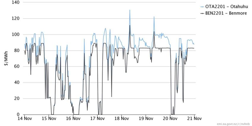
24 November 2021

 Trading Conduct Report
 Market Monitoring Weekly Report

1. Overview for the week of 14 to 20 November
1.1. Energy prices this week appear to be consistent with underlying supply and demand
 conditions. Some trading periods with high reserve prices will be analysed further.

2. Prices
Energy prices
2.1. The average spot price this week was $64/MWh1, 41% lower than last week. Prices were
 below $120/MWh the whole week except for TP17 on 18 November and 19 November
 when prices at Otahuhu were $131/MWh and $122/MWh respectively. There were four
 nights this week when prices collapsed to close to $0/MWh.
Figure 1: Spot prices by trading period at Otahuhu and Benmore

1The simple average of the final price across all nodes, as shown in the trading conduct summary
dashboard

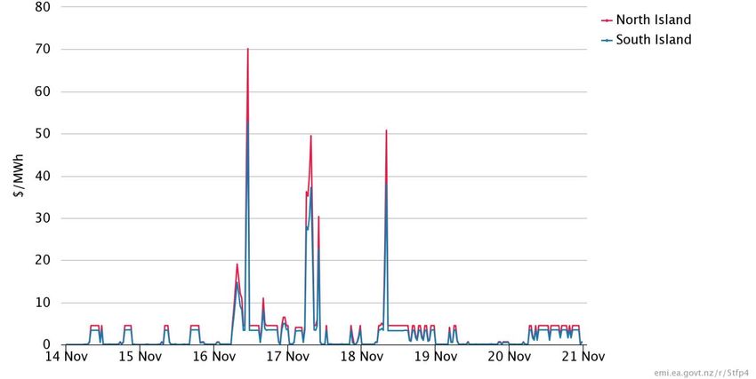
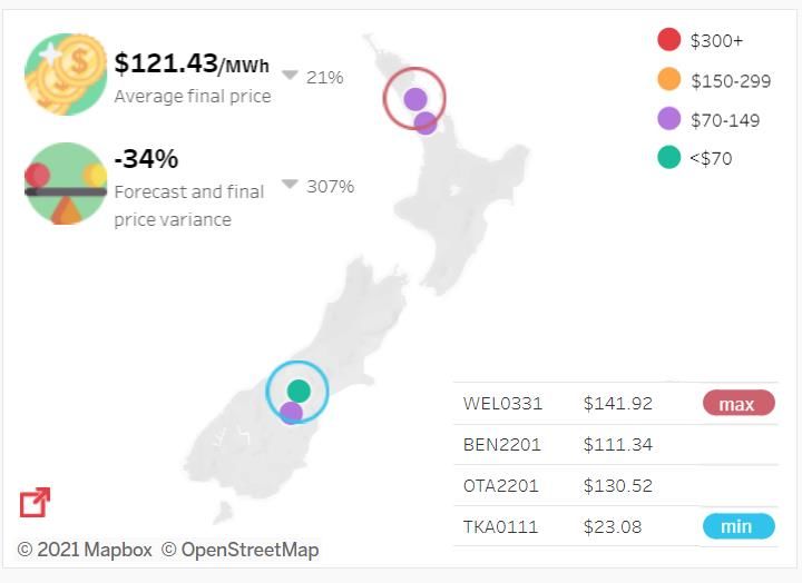
2.2. Figure 2 shows the average price for TP17 on 18 November, the nodal price at Otahuhu,
 Benmore, the highest price node and lowest price node. The average price across nodes
 was 21% lower than the same trading period the week before, indicative of lower prices this
 week. There was price separation between Tekapo A and Benmore due to ongoing
 transmission outages. While this caused lower prices at the Tekapo A node, it unlikely had
 a significant impact on prices due to the small capacity of Tekapo A.
Figure 2: Spot prices for TP17 on 18 November compared to the previous week

Reserve Prices
2.3. Fast instantaneous reserves (FIR) prices were usually below $10/MWh. There were higher
 prices between 16 and 18 November, with the highest price of $70/MWh occurring on TP23
 16 November in the North Island.
Figure 3: FIR prices by trading period and Island

2.4. Sustained instantaneous reserves (SIR) prices were below $25/MWh the entire week (see
 Figure 4), with most prices below $5/MWh. The highest SIR price did coincide with the
 highest FIR price on TP23 16 November.
Figure 4: SIR prices by trading period and Island

Residuals from regression models
2.5. The Authority’s monitoring team has developed two regression models of the spot price.
 The residuals show how close the predicted prices were to actual prices. Large residuals
 may indicate that prices do not reflect underlying supply and demand conditions. Details on
 the regression model and residuals can be found in Appendix A.
2.6. Figure 5 shows the residuals from the weekly model. During October 2021 the residuals
 were within the normal range, indicating that weekly prices were close to the model’s
 predictions.

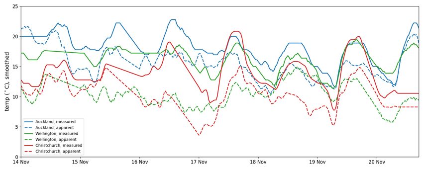
Figure 5: Residual plot of estimated weekly price from 2 July 2019 to 28 October 2021

2.7. Figure 6 shows the residuals of autoregressive moving average (ARMA) errors from the
 daily model. This week the daily residuals were within the normal range.
Figure 6: Residual plot of estimated daily average spot price from 1 July 2020 to 20 November 2021

3. Demand Conditions
3.1. National demand was 3% lower than the previous week (see Figure 7) as warm weather
 continued, particularly in Auckland.

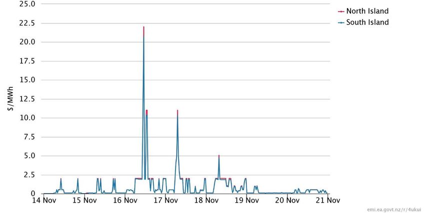
Figure 7: National demand compared for current and previous week

3.2. Figure 8 shows hourly temperature data at main population centres. The measured
 temperature is the recorded temperature, while the apparent temperature adjusts for factors
 like wind speed and humidity to estimate how cold it feels. Warm temperatures continued
 from last week, with Auckland temperatures in particular warmer than last week.
Figure 8: Hourly temperature data (actual and apparent) at main population centres

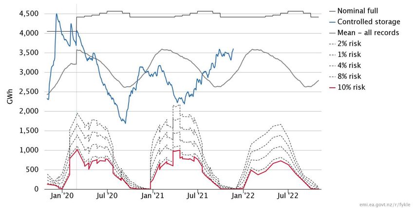
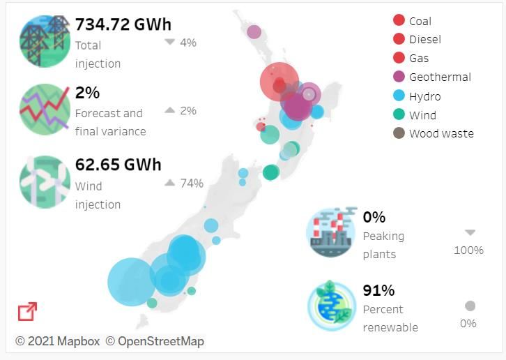
4. Supply Conditions
Figure 9: Generation in the last week compared to previous week

Hydro conditions
4.1. National hydro storage increased this week to 73% of nominal full, shown in Figure 10.
Figure 10: Electricity risk curves and hydro supply

Wind conditions
4.2. Total wind generation was 63GWh, 74% higher than last week. Wind generation was
 particularly high from 14 to 17 November at 400 to 600MW (see Figure 11) which was when
 prices were lowest (particularly overnight). Wind generation was low (below 100 MW) when
 prices were highest on 18 and 19 November.
Figure 11: Wind generation by trading period

Thermal conditions
4.3. Huntly’s E3P continued to run as thermal baseload this week (Figure 12). Huntly unit 4 also
 ran on 18 and 19 November when wind generation was at its lowest and Manapouri had
 several outages.
Figure 12: Generation from baseload thermal by trading period

4.4. Thermal peakers contributed well below 1% of total generation this week, due to low prices
 and high wind. Only Huntly unit 6 briefly ran from TP13 to TP22 on 15 November. Several
 thermal peaker were also on outage, such as Stratford and Junction Road.
Figure 13: Generation from thermal peakers by trading period

Significant outages
4.5. There continues to be a high number of outages this week, most noticeable Manapouri had
 4 units on outage during this week.
4.6. The following outages reduced available generation by at least 50MW:
 (a) Clyde, 116MW (long term outage)
 (b) Benmore, 90MW (5 July – 24 November)
 (c) Manapouri,
 (i) 125MW (7am-4:30pm 14 November)
 (ii) 125MW (15-18 November)\
 (iii) 125MW (16-18 November)
 (iv) 125MW (6am-5pm 17 November)
 (d) Tekapo, 80MW (13 September – 16 January 2022)
 (e) Huntly,
 (i) Rankine unit; 240MW (4 October-19 December)
 (ii) Rankine unit; 240MW (20-21 November)
 (f) McKee, 50MW (17-23 November)
 (g) Maraetai (Waikato River)
 (i) 35.2MW (10-19 November)
 (ii) 35.2MW (11 November -17 December)

(h) Stratford,
 (i) 100MW, (31 October-13 December)
 (ii) 100MW (7-29 November)
 (i) Waipori, 72MW (8 November – 28 January 2022)
 (j) Junction Road,
 (i) 50MW (11-15 November)
 (ii) 50MW (13-16 November)
 (iii) 50MW (16-18 November)
 (k) Aviemore, 55MW (11-26 November)

5. Price versus estimated costs
5.1. In a competitive market prices should be close to (but not necessarily at) the short run
 marginal cost (SRMC) of the marginal generator (where SRMC includes opportunity cost).

Thermal Fuels
5.2. The SRMC (excluding opportunity cost of storage) for thermal fuels can be estimated using
 gas and coal prices, and the average heat rates for each thermal unit. Figure 12 shows
 estimates of thermal SRMCs as a monthly average. The thermal SRMC for both gas and
 coal fuelled generation in November (to 21 November) is similar to October2.
Figure 14: Estimated monthly SRMC for thermal fuels

2For a discussion on these estimates, see our paper ‘Approach to monitoring the trading conduct rule’ at:
https://www.ea.govt.nz/development/work-programme/pricing-cost-allocation/review-of-spot-market-trading-
conduct-provisions/development/trading-conduct-review-decision-published/

DOASA Water values
5.3. The DOASA3 model gives a consistent measure of the opportunity cost of water, by seeking
 to minimise the expected fuel cost of thermal generation and the value of lost load and
 provides an estimate of water values at a range of storage levels. Figure 15 shows the
 national water values4 obtained from DOASA up to end of October 2021. The outputs from
 DOASA closest to actual storage levels are shown as the yellow water value range. These
 values are used to estimate marginal water value at the actual storage level, indicated by
 the blue line5. Figure 15 shows that the marginal water value has declined since June as
 hydro storage levels increased and gas costs decreased.
Figure 15: DOASA water values for January- to November 2021

 Monthly prices
5.4. Figure 16 shows the average price each month at Otahuhu and Benmore for 2021. It shows
 that prices have declined since June, similar to the trend for gas costs and water values.
 The high prices over winter were closer to the SRMC of thermal but as thermal generation
 decreased average prices have been closer to the marginal water value.

3 DOASA is an implementation of the Stochastic Dual Dynamic Programming (SDDP) algorithm of Pereira
and Pinto. DOASA was developed by researchers at the Electric Power Optimisation Centre (EPOC) for the
New Zealand electricity market. (more details in Appendix B)
4 The national water values are estimated assuming all hydro storage reservoirs are equally full.
5 See Appendix B, 2 for more details

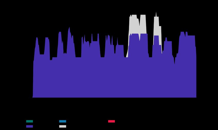
Figure 16: Average monthly prices at Otahuhu and Benmore January-October 2021

Offer Behaviour
Final daily offer stacks
5.5. Figure 13 shows this week’s daily offer stacks, adjusted to take into account wind
 generation, reserves and frequency keeping.6 The black line shows the cleared energy,
 indicating the range of the average final price.
5.6. This week increased wind generation and hydro storage resulted in more generation offered
 between $50-$100/MWh. The quantity of offers above $350/MWh was 6% lower than one
 month ago. Outages did have a noticeable impact on total generation offered some days
 this week.

6The offer stacks show all offers bid into the market (where wind offers are truncated at their actual
generation and excluding generation capacity cleared for reserves) in price bands and plots the cleared
quantity against these.

Figure 17: Daily offer stack

Offers by trading period
5.7. The trading period (TP) with the highest price at Otahuhu was TP17 (8:00am) on 18
 November is shown on Figure 18 as well as the day immediately before on Figure 19. Each
 graph shows the offer stack, the generation weighted average price (GWAP) and cleared
 generation.
5.8. The offer stacks and cleared generation on the two days were similar. However, wind
 generation was almost 200MW lower on 18 November than 17 November which resulted in
 slightly higher prices.
Figure 18: Offer Stack for trading period 17 on 18 November

Figure 19: Offer Stack for trading period 17 on 17 November

Ongoing Work in Trading Conduct
5.9. Some trading periods have been identified this week for further analysis to understand high
 reserve prices.
Table 1: Trading periods identified for further analysis

 Date TP Status Notes
 16/11-18/11 Further Analysis High reserve prices
 30/06-20/08 Several Compliance: review High energy prices in shoulder periods
 30/06-21/08 Several Compliance: review Withdrawn reserve offers

Regression Analysis
1. The Authority’s monitoring team has developed two regression price models. The purpose
 of these models is to understand the drivers of the wholesale spot price and if outcomes are
 indicative of effective competition.

Weekly Model
2. The weekly model is an updated version of the model published in
 https://www.ea.govt.nz/assets/dms-assets/27/27142Quarterly-Review-July-2020.pdf,
 Section 8, pg. 21-25
3. The regression equation is

 where is the PPI and trend adjusted weekly average spot prices; =week 1,…,52 for
 each year; = spring, summer, autumn, and winter

Daily Model
4. The daily model estimates the daily average spot price based on daily storage, demand,
 gas price, wind generation, the HHI for generation (as a measure of competition in
 generation), the ratio of offers to generation (a measure of excess capacity in the market), a
 dummy variable for the period since the 2018 unplanned Pohokura outage started, and the
 weekly carbon price (mapped to daily). The units for the raw data are as following: storage
 and demand are GWh, spot price is $/MWh, gas price is $/PJ, and wind generation is MW,
 carbon price is in New Zealand Units traded under NZ ETS, $/tonne.
5. We used the Augmented Dicky-Fuller (ADF) to test all variables to see if they are stationary.
 If not, we tested the first difference and then the second difference using the ADF test until
 the variable was stationary. The first difference of a time series is the series of changes
 from one period to the next. For example, if the storage is not stationary, we use −
 −1 .
6. We fitted the data using a dynamic regression model with Autoregressive with five lags
 (AR(5)). Dynamic regression is a method to transform ARIMAX (Autoregressive Integrated
 Moving Average with covariates model) and make the coefficients of covariates
 interpretable.
7. Once we dropped the insignificant variables; the ratio of offers to generation, the dummy
 variable for 2018 and carbon price, we got the following model7, where diff is the first
 difference:
 = 0 − 1 ( − 20. . . ) + 2 ( ) −
 3 . + 4 . − 5 ( ) + 6 + 
 = 1 1 − 2 2 + 3 3 + 4 4 + 5 5 + 
8. , the residuals of ARMA errors (from AR(5)), should not significantly different from white
 noise. Ideally, we expect the ARIMA errors are purely random, and are not correlated with
 each other (show no systematic pattern). ARIMA errors equals minus the estimate ̂ with
 their five time lags.

7 Updated, ( ) has been replaced with ( − 20. . . )

DOASA water value model
1. DOASA is an implementation of the Stochastic Dual Dynamic Programming (SDDP)
 algorithm of Pereira and Pinto.8 DOASA was developed by researchers at the Electric
 Power Optimisation Centre (EPOC) for the New Zealand electricity market.9 A version of
 DOASA has been used by EPOC for analysis of the New Zealand electricity market for
 many years, and SDDP is a well known and widely accepted modelling tool for hydro-
 thermal optimisation in electricity systems. DOASA gives a consistent measure of the
 opportunity cost of water. The DOASA model seeks a policy of electricity generation that
 meets demand and minimises the expected fuel cost of thermal generation and value of lost
 load.
2. The DOASA model outputs the marginal water value for a range of storage levels. The
 marginal water value, , at the actual storage level, , is estimated using the outputs closest
 to actual storage level ( 1 , 1 ) and ( 2 , 2 ) using the equation
 − 1
 = 1 + ( )( − 1 )
 2 − 1 2
3. The following are some of the limitations of the assumptions in the DOASA model:
 a. Load is based on forecasts for future periods and recent periods where reconciled
 data was not yet available.
 b. Forecast plant and HVDC outages based on current POCP data
 c. The estimated thermal fuel costs used in DOASA may not accurately represent
 what hydro generators face, in terms of thermal generator offers. Hydro generators
 must manage their storage levels within the context of volatile thermal fuel prices
 and availability, and the thermal fuel cost estimates may not perfectly represent
 these.
 d. Non-dispatchable plant, such as wind, is modelled as having constant power output
 instead of stochastic power output
 e. Some hydro station head ponds and major reservoirs are governed by complex
 resource consent rules. The model limits used in DOASA are necessarily somewhat
 simplified and may not accurately reflect the actual flexibility of these limits.
 f. Inflow probability distributions are based on past inflow sequences.
 g. DOASA does not directly model stagewise dependence (i.e. from week to week) of
 inflows, e.g. if it was wet last week it’s more likely to be wetter this week as well.
 However, DOASA approximates this effect by an approach called Dependent Inflow
 Adjustment (DIA), which artificially increases the variance of historical inflows when
 generating the cutting planes.9
4. We use the average water value over all of New Zealand from DOASA rather than the water
 values for individual reservoirs because the individual reservoir water values are very
 volatile. This is due to the following.
 a. DOASA does a forward solve (linear programming), so as long as the objective
 values are the same, it is likely to use all water from one reservoir first until it hits
 some constraint, before moving to the next reservoir. This leads to the likely
 extreme usage of small reservoirs (ie, not using water proportional to total national
 storage by either holding back or letting it all go).

8 M V Pereira and L M Pinto, “Multi-stage stochastic optimization applied to energy planning,” Mathematical
Programming 52, (1991): 359–375.
9 Electricity Authority, “Doasa overview,” https://www.emi.ea.govt.nz/Wholesale/Tools/Doasa.

b. Therefore, small (constrained) reservoirs in DOASA are expectedly more likely to hit
 maximum or minimum levels or constraints, and this will be reflected in the water
 values (high price if likely to hit minimum level and low price if likely to hit maximum
 level).
c. National water values are calculated based on absolute total national storage, not
 absolute individual reservoir storage, which tends to make the water values less
 volatile. That is, if we had two reservoirs with the same capacity and one had
 storage at 10 percent of capacity and the other at 90 percent, the national water
 value is based on total storage of 50 percent of total capacity