Solving structure from NMR data Analysis 3.0.4 (with Structure alpha) - Picking peaks in NOESY spectra 2. Setting up structure calculations in ...
←
→
Page content transcription
If your browser does not render page correctly, please read the page content below

Solving structure from NMR data
Analysis 3.0.4 (with Structure alpha)

1. Picking peaks in NOESY spectra

2. Setting up structure calculations in Xplor NIH 3.2

3. Analyzing structure calculation results.

4. Assessing protein structure quality.
Solving structure from NMR data
Analysis 3.0.4 (with Structure alpha)
   All materials necessary for this workshop are provided in structure_workshop.zip
   The project we will be using includes backbone and side chain assignments.

1. Picking peaks in NOESY spectra
    There are two approaches to preparing NMR data for structure calculation.
    First, we are going to try automatic peak picking. Some structure calculation programs
    will not use any assignment provided for the peaks and are also particularly suited for
    noisy data, which is an expected result from automatization.

1a. Automatic peak picking
1. Open CCPN Analysis and load structure_1.ccpn project.
       You will see two spectrum displays, N NOESY (SP:n-noesy) spectra in blue and C NOESY
       (SP:c-noesy) in purple and olive.
2. Close SP:n-noesy spectrum for now. Switch to methyl region of the SP:c-noesy spectra by
   typing ‘11.0’ in the Z-navigation toolbar. Inspect SP:c-noesy spectra by going through the Z-
   plane.
3. Double click on the SP:c-noesy on the left-hand menu, raise the contours levels to 650,000 and
   turn of negative contours. Close the pop-up window.
4. Pick peaks in methyl regions. First of all, close all spectrum displays (this speeds things up!).
   then go to ‘Spectrum’ > ‘Pick Peaks’ > ‘Pick ND Peaks…’ and pick the following three regions
   using “Positive only”:
       Region 1:
       'Hc': 0.0 - 1.5
       'H': 0.0 - 10.05
       'Ch’: 10.0 – 15.0
       Region 2:
       'Hc': 0 - 2.6
       'H': 0.0-10.05
       'Ch’: 22 – 26
       Region 3:
       'Hc': 3.0 - 4.7
       'H': 0.0-10.05
       'Ch': 50 – 54

5. Water signal between 4.7 – 5 ppm in Hc (x) dimension stretches through the whole the spectra.
   Go through the z-dimension and identify other regions which should be avoided in automatic
   peak picking.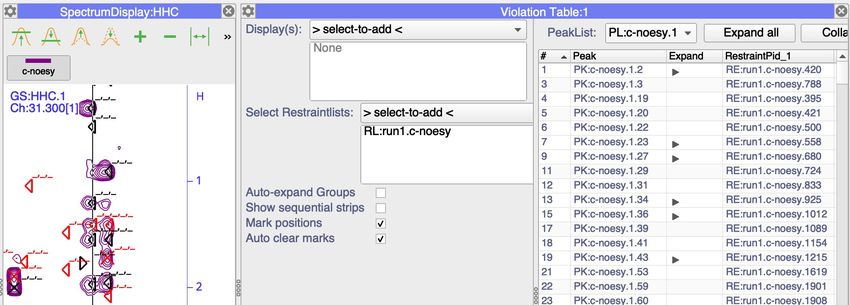
1b. Manual picking and assigning of N-NOESY peaks
In the other approach we will now hand pick and assign some of the N-NOESY picks using
strip plots. Peaks can be picked from their roots in N- or C-HSQC spectra. Some programs
handle structure calculation better with some initially assigned peaks. In particular, if
secondary structure elements such as alpha helical regions can be predicted, it is often
possible to assign sequential NH-NH peaks in the N-NOESY spectrum. This protein has alpha
helical regions between residues 10 – 20, 29 – 39 and 50 – 63 and we can assign sequential
crosspeaks in these regions.
1. Close SP:c-noesy spectrum display and drag SP:n-noesy and SP:hsqc to Drop Area.
2. Go to Main Menu > ‘Assign’ > ‘Pick and Assign’.
3. Open gear box setting of the Pick and Assign module. Add GD:HHN in the ‘Navigate to
Display(s)’ scroll down menu and close the settings.
4. Select NC:A in the NmrChain scroll down menu.
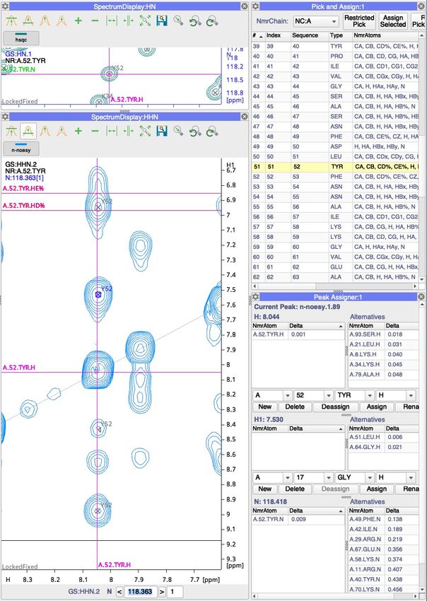
5. Double click on 52 TYR row. You will see n-noesy spectrum moving to the HN 52 TYR position.
6. Pick peaks by Shift+Cmd(Ctrl)+Drag along the marked strip, you may need to change the z-
plane slightly.
7. With peaks selected along the 52 TYR HN strip click ‘Assign Selected’ button in Pick and Assign
module, this will assign peaks to 52 TYR.
8. Go to Main Menu > ‘Assign’ > ‘Peak Assigner’ (shortcut ‘AP’)
9. Click on the peak just above the diagonal of the 52 TYR strip:
1. CLICK
2. DOUBLE CLICK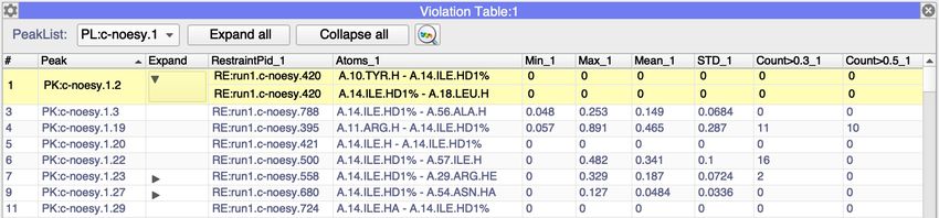
1b. Manual picking and assigning of N-NOESY peaks continue

10. You can observe that one of the options for assigning the H1 dimension is 51 LEU. Double click
    will assign the A.51.LEU.H to this peak dimension.
11. Add another strip to the spectrum display (green plus sign on the toolbar).
12. Double click on the next raw with 53 PHE in the Pick and Assign module. This will move spectra
    in the next active strip to NH position for 53 PHE. Pick and assign the peaks as for 53 PHE.
13. Add another strip, double click on the row with 54 ASN. You can observe that there is much
    more overlap in this strip and assigning peaks is more challenging. Can you identify any
    sequential crosspeaks?
14. Starting from 16 GLU try to assign sequential peaks in this helical region.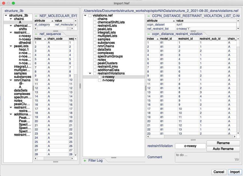
2. Setting up structure calculations in Xplor NIH 3.2
  Once both N- and C-Noesy peak lists are ready we can export NEF file with all information
  needed to perform structure calculation. Using macro we will set up a folder in which all
  Xplor NIH scripts needed for driving calculation will be stored as well. You can follow demo
  steps if you have installed Xplor NIH and TalosN on your computer, otherwise you can use
  folders that are already prepared in the workshop material.

2a. Setting and running Xplor NIH
  In the CCPN project used for this part of tutorial peaks were picked automatically and
  diagonal peaks were removed using macro deleteDiagonalPeaks.py. It can be found in
  …/structure_workshop/scripts. Macro can be run by ‘Macro’ > ‘Run…’ and selecting python
  file from above location.
1. Open CCPN Analysis and load structure_2.ccpn project.
2. Go to ‘Project’ > ‘Preferences’. In the resulting pop-up, go the ‘External Programs’ tab and put
   in the paths to the software. Click OK to close the window. The paths should look like:
       /Users/user1/programs/talosn/talosn
       /Users/user1/programs/xplor-nih-3.2/bin/xplor
3. We can also set up path for Pymol, which we will need later.
       On Mac this will be on: /Applications/MacPyMOL.app/Contents/MacOS/MacPyMOL
4. Go to ‘Main Menu’ > ‘Macro’ > ‘Run CCPN Macro’ > ‘SetupXplorStructureCalcPopup’
5. You will see po-up showing up:

6. Set to the ‘Xplor Run Directory’ to the location where you want your calculation folder to be
   created and in which the output of the calculation will be saved. Either type the directory in by
   hand, or use the icon to navigate there using the file browser.
7. Remove PL:hsqc.1 from ‘Included’ PeakLists by dragging it to ‘Not included’, leaving only PL:n-
   noesy.1, PL:c-noesy.1 as ‘Included’.
8. As the prepared project has only one chemical shift list and one Chain you do not have to
   change these.
9. Click Setup to run the Macro.
       This will create a directory in your specified location.
10. Go to the location you specified in the macro pop-up.
        You should have a folder called ‘structure_2_2021-05-05’ which should list following:
        - CCPN_H1GI_clean.nef, README, fold.py, genTalosNInput.py, initMatch3d.py,
        jointFilter.py, makeNEF.py, nef2xplor.py, pass2.py, pass3.py, runTalos.sh,
        summarize_pass2.py, summarize_pass3.py, talosToNEF.py – files copied from Xplor NIH,
        scripts for controlling each part of the calculations.
        - ‘structure_2.nef’ - NEF file containing chain, chemical shift list, n-noesy and c-noesy
        peak lists.
        - ‘runxplor_structure_ 2_2021-08-20.sh’ - shell script for running calculation.
11. To start calculation, you need to execute the script (by typing: ./runxplor_structure_2_2021-
    05-05.sh) in the terminal window in the set-up folder.
        These calculation are computationally very intensive; it is therefore advisable to run
        them on a multiprocessor system, if possible.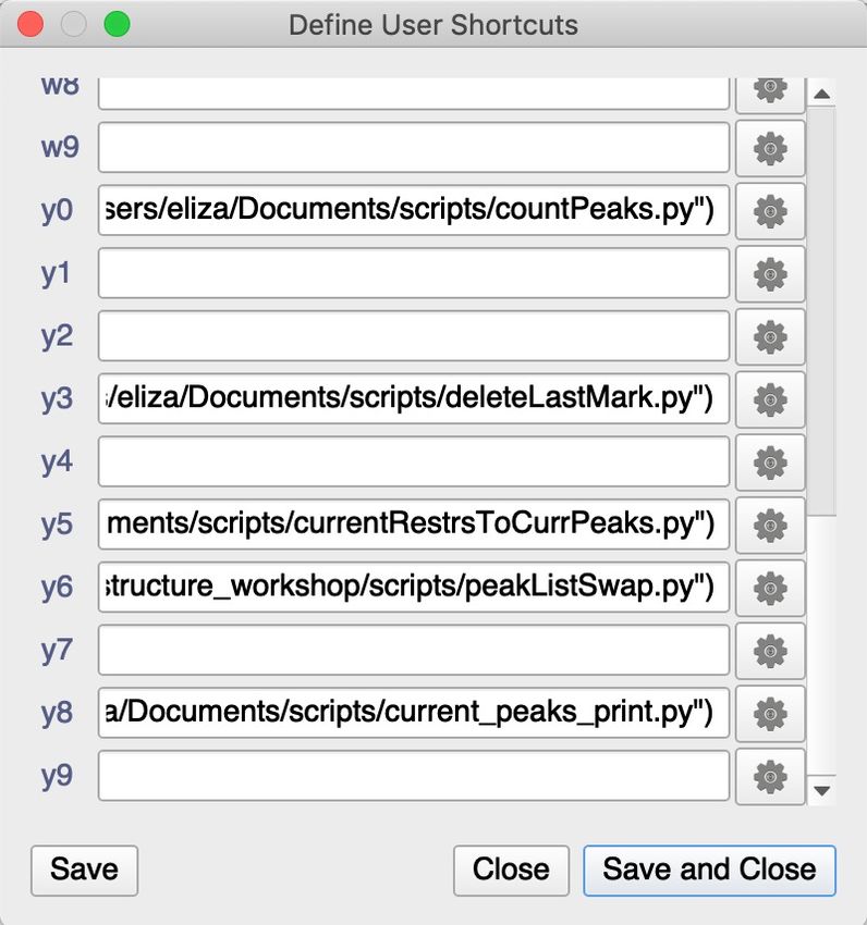
3. Analyzing structure calculation results.
     As the calculation can take a long time to complete, we have provided a folder with
     results that are already organized into subfolders, which can be done with a macro.

3a. Processing results of Xplor NIH structure calculation
     All files resulting from Xplor NIH calculation are output in one folder. To help navigate
     through this folder you can run a CCPN macro (processXplorNIHCalculation). This macro
     will sort files into appropriate folders, create NEF file where Xplor comments are
     removed (structure_2_2021-08-20_out.nef) and in addition it will generate
     ensemble.pdb file with lowest energy models, which you can view in Pymol.

     You can skip this part during tutorial, the processed folder can be found at:
     …/structure_workshop/xplorNihData/structure_2_2021-08-20_done

1. Go to the Main Menu > ‘Macro’ > ‘Run CCPN Macro’ > ‘processXplorNIHCalculation’
2. From resulting pop out window navigate to
   …/structure_workshop/xplorNihData/structure_2_2021-08-20
3. Click ‘Clean Up’. When the process is complete you will see a pop up with a message ”Clean up
   complete!”, press OK.

3b. Assessing structure in molecular viewer
     The first step when analyzing results should be inspecting the structure models in
     molecular viewer ensuring all models are inspected.

1.   Open Pymol
2.   Go to …/structure_workshop/xplorNihData/structure_2_2021-08-20_done/fold.
3.   Drop ensemble.pdb onto your opened Pymol window.
4.   To have a better view on the structure you may execute following commands in command
     input:

        dss
        show cartoon
        hide lines
        set all_states, 1
        set seq_view, 1
        util.cbam ss h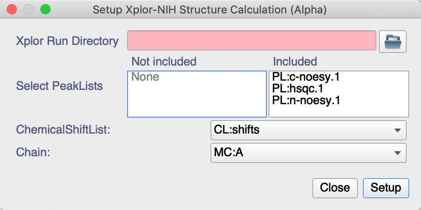
3c. Loading NEF file with generated restraints
1. With structure_2.ccpn project open go to ‘Project’ > ’Import’ > ‘Nef File, in the resulting
   window select: …/structure_workshop/xplorNihData/structure_2_2021-08-
   20_done/structure_2_2021-08-20_out.nef
2. After a moment you will see a pop-up window of the Nef Importer:

                                        CLICK

4. Click on ‘1’ in restraintLists, this will highlight this part of structure_2_2021-08-20_out.nef.
   Type in new name and click ‘Rename’ to confirm:

5. Select restraintLists and restraintLinks and click ‘Import’.

6. You will now have the restraints inside the project listed under DataSets in the left-hand menu.
   To rename it, double click on DS:myDataSet_1, in the Edit DataSet pop-up window change the
   name to ‘run1’.
7. At this stage it is useful to mark peaks that have been rejected and accepted during the
   calculation, it can be done with CCPN Macro (‘Main Menu’ > ‘Macro’ > ‘Run CCPN Macro’ >
   ‘SplitPeaksToRejectedAndAccepted’). This will create new peak list (with comment ‘rejected’)
   and peaks coloured red, first peaks list (PL:c-noesy.1) will have comment “accepted” added.

8. We can display restraints on the lowest energy structure model in Pymol. Make sure the Pymol
   path is set in the ‘Project’ > ‘Preferences’.
9. Double-click on the c-noesy RestraintList under DataSets’ DS:run1 in the sidebar to give you the
   ‘Edit RestraintList’ pop-up.
   The ‘Molecule FilePath’ should point to the
   …/structure_workshop/xplorNihData/structure_2_2021-08-
   20_done/fold/lowestEnergyStructure.cif file on your computer.

                                                DOUBLE
                                                CLICK

10. Repeat for the 'RL:run1.n-noesy'

3d. Loading violations in NEF format.
    In the current 3.0.4 AnalysisAssign version processing violations from Xplor NIH calculations is
    not completely streamlined and substantial changes are coming in 3.1.0 version.
    For the purpose of this tutorials we have generated file with violations
    (…/structure_workshop/xplorNihData/structure_2_2021-08-20_done/violations.nef)

    If you with to prepare this file yourself instructions are available at the end of this tutorial.

1. Go to ‘Project’ > ’Import’ > ‘Nef File, in the resulting window select:
   …/structure_workshop/xplorNihData/structure_2_2021-08-20_done/violations.nef
2. After a moment you will see a pop-up window of the Nef Importer: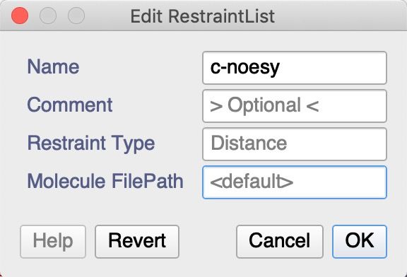
3. Select both c-noesy and n-noesy restraintViolations and click ‘Import’.
       This may take a few minutes as the file is very large.
4. Once violations are loaded in the project we need to link them to the restraints and generate
   average violations for each restraint. In current version this is achieved by a macro. Go to ‘Macro’ >
   ’Run CCPN Macros’ > calculateViolationAverage.
       This may again take few minutes.

3e. Analyzing violations
     In the initial steps of structure calculation runs in is the important to go through violated
     restraints and inspect the peaks they originate from. This, together with surveying
     rejected peaks, is the most time-consuming process in the structure calculation.
1.    Drag 'SP:c-noesy’ into the Drop Area to display it.
2.    Go to ‘Main Menu’ > ‘View’ > ‘Violation Table’. In the PeakList: pull down menu select
      'PL:c-noesy.1’. Open the Settings using the gear box icon and select Display(s) select
      GD:HHC and in Select Restraintlists: add 'RL:run1.c-noesy’ (it should look as in the
      picture below). Close the gear box.
6. As the restraints, violations were linked with the peaks double click on the row of the table will
select peak on the spectrum display.
7. You can sort the table to view the most violated restraints by clicking on either Max_1 or
Mean_1 column head.
8. Expand column allows you to view contributions from ambiguous restraints.
9. To view only restraints violated in more then 10 structures right click on column heads:
At the bottom of the table you will see selection box where you can input appropriate
values:
10. You can use the same filter box to find restraints to a particular residue, for instance 52 Tyr:
11. If you also inspect restraints on structure model. Select all restraints (rows) you wish to view on
click on the structure button on the top of the table.
Every click on the button will open new Pymol pop up.12. If you identify peaks you want to move from peak list 1 (accepted peaks) to peak list 2 (or the
pother way round) convenient way of doing is to have keyboard shortcut. You can link
.../structure_workshop/scripts/peakListSwap.py macro to a keyboard shortcut. Go to ‘Macro’ >
‘Define Macro Shortcuts…’.
13. Click on the gear box button next to your chosen shortcut on navigate to the location on your
computer.
This macro will work well if you only have two peak lists associated with your spectra, one
for accepted peaks, and one for rejected ones.
14. Cick Open and then Save and Close
15. When peak is selected pressing keyboard shortcut should trigger color change indicating
moving peaks between lists.
3f. Analysis results from multiple structure calculation runs
You can add more restraint lists to the Violation Table. You can find subsequent run for
this protein data in …/structure_workshop/xplorNihData/structure_3f_2021-08-
23_done.
Project ready with both run result loaded (including violations) can be found in:
…/structure_workshop/structure_3f.ccpnFormatting violations.
Python script was written by Dr Gary Thompson (CCPN, University of Kent) and modified in
few places.
1. You will need to install Python libraries listed in the script.
2. Open file fold_##.sa.stats located in …/structure_workshop/xplorNihData/structure_2_2021-
08-20_done/fold.
3. At the end of the file there is a list with the lowest energy structures (all those files are in the
folder ). For each of the structures (for example fold_91.sa) there is a .viols file listing violations
for this model (fold_91.sa.viols).
4. To generate violations.nef file for the lowest energy set run in terminal in
…/structure_workshop/xplorNihData/structure_2_2021-08-20_done/fold/lowestEnergy folder:
> viols_to_nef.py -o violations.nef fold_91.sa.viols fold_77.sa.viols fold_11.sa.viols
fold_44.sa.viols fold_74.sa.viols fold_68.sa.viols fold_86.sa.viols fold_14.sa.viols
fold_70.sa.viols fold_26.sa.viols fold_63.sa.viols fold_57.sa.viols fold_97.sa.viols
fold_15.sa.viols fold_37.sa.viols fold_50.sa.viols fold_52.sa.viols fold_69.sa.viols
fold_36.sa.viols fold_23.sa.viols
5. This will generate violations.nef in this folder.
6. In order to link the violation from this file to the restraints in the project (stored in DateSet
DS:run1) you need to add a tag in the saveframe of the file:
_ccpn_distance_restraint_violation_list.ccpn_dataset run1
_ccpn_distance_restraint_violation_list.run_id run_test_01
Resulting saveframe should look like this with added lines:
Repeat this process for _ccpn_distance_restraint_violation_list_n-noesy`1` saveframe.You can also read