Multi-method approach shows stock structure in Loligo forbesii squid
←
→
Page content transcription
If your browser does not render page correctly, please read the page content below
ICES Journal of Marine Science, 2022, 0, 1–16
DOI: 10.1093/icesjms/fsac039
Original Article

Multi-method approach shows stock structure in Loligo
forbesii squid
Edel Sheerin1,† , Leigh Barnwall1,† , Esther Abad2 , Angela Larivain3 , Daniel Oesterwind 4 ,

                                                                                                                                                             Downloaded from https://academic.oup.com/icesjms/advance-article/doi/10.1093/icesjms/fsac039/6551738 by guest on 22 March 2022
Michael Petroni1 , Catalina Perales-Raya5 , Jean-Paul Robin3 , Ignacio Sobrino6 , Julio Valeiras2 ,
Denise O’Meara7 , Graham J. Pierce8 , A. Louise Allcock 1 and Anne Marie Power 1,*
1
  Ryan Institute, School of Natural Sciences, National University of Ireland Galway, H91 TK33 Galway, Ireland
2
  Instituto Español de Oceanografía, Centro Oceanográfico de Vigo, 36390 Vigo, Spain
3
  BOREA: Biologie des ORganismes et des Ecosystèmes Aquatiques, Université de Caen Normandie, 14032 Caen, France
4
  Thünen-Institut of Baltic Sea Fisheries, D-18069 Rostock, Germany
5
  Instituto Español de Oceanografía, Centro Oceanográfico de Canarias, 38180 Santa Cruz de Tenerife, Spain
6
  Instituto Español de Oceanografía, Centro Oceanográfico de Cádiz, 11006 Cádiz, Spain
7
  Molecular Ecology Research Group, Eco-innovation Research Centre, School of Science and Computing, Waterford Institute of Technology,
Waterford, X91 K0EK, Ireland
8
  Instituto de Investigaciones Marinas (CSIC), Eduardo Cabello 6, 36208 Vigo, Spain
* Corresponding       author: tel: +353 91 493015; e-mail: annemarie.power@nuigalway.ie.
†
    co-first author

Knowledge of stock structure is a priority for effective assessment of commercially-fished cephalopods. Loligo forbesii squid are thought to
migrate inshore for breeding and offshore for feeding and long-range movements are implied from past studies showing genetic homogeneity in
the entire neritic population. Only offshore populations (Faroe and Rockall Bank) were considered distinct. The present study applied mitchondrial
and microsatellite markers (nine loci) to samples from Rockall Bank, north Scotland, North Sea, various shelf locations in Ireland, English Channel,
northern Bay of Biscay, north Spain, and Bay of Cadiz. No statistically significant genetic sub-structure was found, although some non-significant
trends involving Rockall were seen using microsatellite markers. Differences in L. forbesii statolith shape were apparent at a subset of locations,
with most locations showing pairwise differences and statoliths from north Ireland being highly distinct. This suggests that (i) statolith shape
is highly sensitive to local conditions and (ii) L. forbesii forms distinguishable groups (based on shape statistics), maintaining these groups
over sufficiently long periods for local conditions to affect the shape of the statolith. Overall evidence suggests that L. forbesii forms separable
(ecological) groups over short timescales with a semi-isolated breeding group at Rockall whose distinctiveness varies over time.
Keywords: ecological stocks, genetics, Loligo, microsatellite, Rockall, statolith shape.

Introduction                                                                         to the south as far as west Africa (Senegal, mainly north of
In the recent years, there has been a global expansion in                            24ºN) and north to the Faroe Islands, and also inhabits much
cephalopod fisheries as conventional finfish stocks are de-                          of the Mediterranean (Guerra et al., 2014; Jereb et al., 2015).
pleted (Caddy and Rodhouse, 1998; Hunsicker et al., 2010;                            Most parts of its distribution overlap with the closely re-
Arkhipkin et al., 2021). This trend has been less pronounced                         lated and commercially valued L. vulgaris, but the relative
within the North East Atlantic, where the bulk of cephalo-                           importance of L. forbesii in landings from Spanish and Por-
pod (and especially squid) landings are a result of bycatch                          tuguese Atlantic coasts declined markedly in the 1990s and
during demersal fishing activities (Howard et al., 1987; ICES,                       2000s (Chen et al., 2006). Although L. forbesii is caught
2020). Nevertheless, even here, an increasing number of ves-                         commercially throughout much of its distribution, including
sels have, from time-to-time, supplemented their standard fish-                      directed artisanal fisheries in Iberia; the Moray Firth and
ing with seasonally directed squid fishing (Young et al., 2006;                      Rockall are amongst the few areas that support targeted trawl-
Arkhipkin et al., 2015). The veined squid (Loligo forbesii) is                       ing fisheries (Pierce, et al., 1994a; Young et al., 2006), with
among several commercially valued species of cephalopod in                           landings in other areas primarily being from bycatch fisheries
the North East Atlantic, which experiences steady levels of                          (Young et al., 2006).
fishing pressure due to its respectable market value and sta-                           Like most squid, L. forbesii completes its short life-cycle
tus as a non-quota species. Landings are typically reported                          within a maximum of 16 months but rarely takes more
together with other long-finned squid species (including L.                          than 12 months (Guerra and Rocha, 1994). The popula-
vulgaris and Alloteuthis spp.), which together have landings                         tion(s) and the fishery landings, thus, tend to show a fairly
of ∼8000–12 000 tonnes per year, with French, Portuguese,                            consistent annual cycle—although at longer scales there is
Spanish, and the UK fleets accounting for > 90% of the catch                         some evidence of shifts, possibly related to differing propor-
(Hastie et al., 2009; ICES, 2020). Loligo forbesii is distributed                    tions of winter and summer breeders (Pierce et al., 2005).
in neritic waters throughout much of the North East Atlantic,                        This species also displays a rapid growth rate with younger

Received: August 30, 2021. Revised: December 10, 2021. Accepted: February 4, 2022

C The Author(s) 2022. Published by Oxford University Press on behalf of International Council for the Exploration of the Sea. This is an Open Access

article distributed under the terms of the Creative Commons Attribution License (https://creativecommons.org/licenses/by/4.0/), which permits unrestricted
reuse, distribution, and reproduction in any medium, provided the original work is properly cited.
2                                                                                                                   E. Sheerin et al.

individuals capable of increasing in size by up to 8% of their     individuals with wide-ranging movements, noting that indi-
own body weight daily (BW/d) under captive conditions, un-         viduals are capable of moving to spawning sites >200 km
til maturity, by which time growth rate decreases to 2%–4%         away within 18 days. Similarly, the population of Doryteuthis
BW/d (Forsythe and Hanlon, 1989). Individuals typically die        opalescens, has two spawning grounds, one in northern Cal-
after spawning, i.e. they are semelparous (Lum-Kong et al.,        ifornia and one in southern California, but despite this, sam-
1992; Boyle and Ngoile, 1993), however spawning can take           ples across a large area from British Columbia to Mexico were
place in several batches over a period of time—a life his-         genetically homogenous (using six microsatellite DNA loci),
tory strategy termed “intermittent terminal spawning” (Rocha       indicating that geographical barriers to gene flow were absent
et al., 2001). In northern Europe, Loligo forbesii spawning        along ≈ 2500 km of coastline (Reichow and Smith, 2001).

                                                                                                                                        Downloaded from https://academic.oup.com/icesjms/advance-article/doi/10.1093/icesjms/fsac039/6551738 by guest on 22 March 2022
grounds are thought to exist along the coast of Scotland, the      Thus, even when ecological differences exist (discrete spawn-
North Sea, west of Ireland and into the western Celtic Sea         ing areas, in this example), populations can constitute a single
(Collins et al., 1995; Laptikhovsky et al., 2021). Consistent      genetic stock.
with it being semelparous, Loligo forbesii, like many squid,          Under a more “ecological” stock concept, a stock may be
has non-overlapping generations, such that recruitment of          considered a management unit or group of individuals which
each successive generation is totally dependent on the survival    are characterised by similarities that are not necessarily inher-
and successful reproduction of the previous one (Boyle, 1990).     ited or related to an isolated breeding group, but include those
However, this comes with a temporally spaced-out spawn-            induced by the environment (Begg and Waldman, 1999; Begg
ing and recruitment period (indeed, possibly also winter and       and Brown, 2000). Hence group similarities might be based
summer spawning seasons (Pierce et al., 1994a; Boyle et al.,       on shared phenotypes or phenological factors (spawning pe-
1995)), which acts as a sort of “bet-hedging” strategy to avoid    riod, for instance). These factors can be linked and are often
catastrophic loss of spawning stock or recruits in each cycle      biologically meaningful, for example: groups of fish can be
(Caddy, 1983). At the same time, this species is potentially       identified with phenotypic similarities (otolith widths) that are
susceptible to recruitment overfishing whereby individuals are     associated with biological characteristics (different juvenile
removed from the stock before they can reproduce, to the           growth rates, indicated in the otolith) caused by phenological
detriment of future recruitment (Collins et al., 1997). This is    factors (autumn- versus winter-spawning adult stock) (Burke
particularly true where knowledge is lacking on how the pop-       et al., 2008). This approach not only helps define a stock,
ulation may be segregated spatially, with the possibility that     but provides critical information for stock management since
more isolated components of the metapopulation (i.e. those         less productive stock components (lower growth rates) cannot
which receive few recruits from outside) could be over-fished.     be sustainably exploited at the same rate as more productive
An example of this is the Rockall population, which is ex-         stock units (Begg et al., 1999). This broader stock definition
ploited by a directed fishery (ICES, 2020) but is partially iso-   also includes ecological characteristics such as shared feeding
lated from other stocks (Shaw et al., 1999) and is believed to     grounds, shared nursery grounds or shared migrations. The
have undergone localised stock depletions in the past (Young       latter are also relevant for management since stock exchange
et al., 2004).                                                     between particular geographical areas must be known to man-
    Knowledge of stock structure is generally poor for com-        age changes in abundance due to migration (Begg et al., 1999;
mercially fished cephalopods, making this a priority research      Power et al., 2005).
area (Jereb et al., 2015; Lishchenko et al., 2021), however,          Under the ecological stock definition, a wider range of tools
stock structure has been assessed previously in L. forbesii us-    to investigate stock structure become available and a multi-
ing various methods. Allozymes and other molecular methods         disciplinary approach combining several tools can be help-
showed no genetic structure along the European continental         ful. For example, Van der Vyver et al. (2016) undertook a
shelf locations (including Rockall and Faroe banks) but the        combined genetic (microsatellite, four loci) and morphome-
Azores samples were sufficiently different to warrant consid-      tric study of L. reynaudii in similar locations to Shaw et al.’s
eration as a subspecies (Norman et al., 1994; Brierley et al.,     (2010) study (see above), where they confirmed no signifi-
1995). More sensitive microsatellite DNA markers concluded         cant population genetic structure. However, it was possible
that the North East Atlantic population is panmictic with the      to distinguish phenotypic differences among genetically ho-
exception of two areas: Rockall and Faroe Banks (Shaw et           mogenous groups. Morphometric variation (43 variables on
al., 1999). This was attributed to the highly migratory nature     the body, beak, gladius, statolith) was observed in samples
of this species, enabling gene flow between different areas, ex-   from either side of Cape Agulhas and south Angola. This was
cept where these were segregated by isolating oceanographic        attributed to environmental influences on growth and body
regimes and expanses of deep water, as seen in Rockall/Faroe       shape, which differed between groups (Van der Vyver et al.,
Banks (Shaw et al., 1999). Because populations can share           2016). Morphometric analysis of body shape (Silva, 2003) or
spawning grounds but can be found in discrete units outside        hard structures (Campana and Casselman, 1993; Libungan et
of the spawning period, genetic characteristics do not give a      al., 2015a) can frequently indicate differences in phenotype.
full picture regarding the “stock concept” and important in-       Since squid are soft-bodied organisms, full body morphomet-
formation can be gained by including non-genetic markers           ric analyses are difficult in this group, though not impossible
(Begg et al., 1999). To illustrate the issue with genetic mark-    (see Pierce et al., 1994b; Pierce et al., 1994c; Van der Vyver et
ers: Shaw et al. (2010) performed microsatellite DNA analysis      al., 2016; Jones et al., 2019). Studies involving hard parts such
(eight loci) on separate spawning groups in Loligo reynaudii       as beaks, gladii (i.e. internal chitinous shells) and statoliths
over an area spanning East to West Cape in South Africa, and       have provided promising results. For example, changes in iso-
found little evidence of genetically separate populations. An      tope signatures (δ 13 C and δ 15 N) from the conus of the gladius
explanation was provided by Sauer et al. (2000), who un-           to its postracum edge revealed ontogenic migrations in Illex
dertook a tagging study of Loligo reynaudii in the same area       argentinus and Doryteuthis gahi (Rosas-Luis et al., 2017) and
and provided evidence that spawning grounds are shared by          in Ommastrephes bartramii (Kato et al., 2016). This approach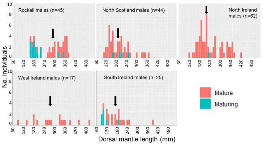
Multi-method approach shows stock structure in Loligo forbesii squid                                                                                           3

Table 1. Sample location details and basic genetic diversity indices including the average no. of individuals genotyped at each locus (Ng ), the no. of alleles
(Na ), observed (Ho ) and expected (He ) heterozygosities, the fixation index (F), the inbreeding co-efficient (FIS ), and allelic richness (Ar ).

Sample location                  Code       Year and Quarter         Sample size        Ng         Na         Ho         He          F         FIS       Ar

North Scotland (NS)                1             19 Q4                    27           25.9       13.9      0.790      0.868      0.088      0.109       9.5
Rockall (RK)                       2             19 Q3                   36           35.6        14.9      0.814      0.860      0.050      0.066       9.3
North Ireland (NI)                 3        18 Q4/19 Q1,Q4               149          143.4       19.9      0.796      0.878      0.094      0.098       9.7
West Ireland (WI)                  4         18 Q4/19 Q1                 53            52.4       16.2      0.803      0.866      0.074      0.083       9.5
South Ireland (SI)                 5          18 Q1/18 Q4                 45           44.8       17.6      0.815      0.872      0.064      0.076       9.9
North Sea (NSea)                   6             19 Q1                   13            12.8       11.2      0.778      0.859      0.093      0.134       10

                                                                                                                                                                   Downloaded from https://academic.oup.com/icesjms/advance-article/doi/10.1093/icesjms/fsac039/6551738 by guest on 22 March 2022
English Channel (ECh)              7             19 Q3                   29            28.7       13.9      0.809      0.868      0.069      0.086       9.5
North Spain (NSp)                  8             19 Q3                   25            24.9       13.3      0.804      0.860      0.061      0.086       9.4
Cadiz (Cad)                        9             19 Q4                    25           23.7       13.1      0.771      0.852      0.091      0.117       9.3
Bay of Biscay (BB)                10             19 Q4                    23           20.4       13.3      0.838      0.873      0.041      0.068       10
Mean                                                                                              14.7      0.802      0.866

can also be used to map ontogenic migrations according to                          microsatellites) at ten locations spanning south Iberia to the
changes in the trophic niche (Kato et al., 2016; Rosas-Luis                        north of Scotland and Rockall. In tandem, comparisons of
et al., 2017), or can be used to understand inshore–offshore                       statolith shape—an ecological stock marker, and biological
migrations when seawater isotopic signatures differ between                        data (length distribution, maturity and sex ratio), were con-
habitats (Dance et al., 2014). The analysis of migration pat-                      ducted at a sub-set of five locations to the north of the range.
terns from statolith elemental signatures can also be combined                     Biological data were included to provide a starting point
with statolith shape analysis to discriminate stocks (Green et                     for interpreting groupings indicated by other stock markers.
al., 2015; Jones et al., 2018a).                                                   The results of this study are intended to indicate the spa-
   Statoliths are paired calcified deposits located in the head,                   tial scale at which separate units of stock may be distin-
and are the cephalopod’s primary balance organ (Young,                             guished in L. forbesii and to interpret these in light of previous
1989). The morphology of statoliths is unique to each species                      research.
and these structures contain valuable ecological and life his-
tory information, acting as “black box” life recorders (Arkhip-
kin, 2005). The morphology of statoliths can vary between                          Methods
cephalopods inhabiting different habitat types (e.g. demer-                        Genetic sample collection
sal versus pelagic) due to this organ’s involvement in accel-
                                                                                   Samples from a total of 425 individuals were collected from
eration and gravity reception (Arkhipkin and Bizikov, 2000).
                                                                                   10 locations in the North East Atlantic (see Table 1 and
As with the equivalent structures in fish (otoliths), care must
                                                                                   Figure 1). All samples were taken aboard research surveys,
be taken in interpreting morphologies from different groups,
                                                                                   with the exception of one sampling location (English Chan-
since otoliths have been shown to vary between age groups,
                                                                                   nel) where samples were obtained via port sampling. To ob-
sexes (Campana and Casselman, 1993), and genotypes (Vi-
                                                                                   tain reasonable sample sizes (Hale et al., 2012), individu-
gnon and Morat, 2010). Analysis of statolith/otolith shape
                                                                                   als sampled from multiple research surveys and sampling
is nowadays carried out using “geometric morphometrics,” a
                                                                                   years/seasonal quarters were grouped to comprise each sam-
term coined to describe analysis of point co-ordinates in two
                                                                                   pling “location,” assuming that these came from stations that
or three dimensions (Marcus and Corti, 1996; see Adams et
                                                                                   were judged to be sufficiently close together. A full breakdown
al., 2004 for a review). Semi-automated shape analysis meth-
                                                                                   of spatially referenced sampling stations and survey informa-
ods have recently been developed, including software to de-
                                                                                   tion is provided in Supplementary Table S1. Tissue sampling
compose an outline (shape) into a series of representative
                                                                                   took place after sorting of the catch by species on-board each
coefficients, which has become widely used due to its accuracy,
                                                                                   research survey, or in the case of port samples, after returning
robustness and speed (Libungan and Pálsson, 2015). Using
                                                                                   to the laboratory. Mantle tissue samples were taken after first
such semi-automated techniques, statolith shape variations
                                                                                   removing the skin, and tissue was transferred to 2 mL Eppen-
have been observed in Humboldt squid (Dosidicus gigas) sam-
                                                                                   dorf tubes containing 96% ethanol. All tissue samples were
pled from different areas, which were consistent across sam-
                                                                                   stored at −20◦ C.
pling years (no statistical stock x year interaction), however,
the spatial scale examined was rather large, spanning 50 de-
grees of latitude (Fang et al., 2018). If this technique could also                DNA extraction and COI Analysis
distinguish stock groupings in neritic species and at smaller                      DNA was extracted using the Invitrogen™ PureLink™ Ge-
spatial scales, this would offer a rapid method of distinguish-                    nomic DNA Mini Kit, following the Mammalian Tissue and
ing ecological stocks since the shape analysis itself can be semi-                 Mouse/Rat Tail Lysate protocol. DNA was eluted in 100 μL
automated. This approach could inform about areas/species                          Genomic Elution Buffer and stored at –20◦ C.
where different ecological groupings can be distinguished, de-                        DNA barcoding, which targets the 650 bp frag-
spite a degree of mixing at some stage in the lifecycle to make                    ment of the COI gene, was performed using forward
genetic sub-structuring undetectable.                                              LCO1490:       5 -GGTCAACAAATCATAAAGATATTGG-3
   The objective of the current study was to apply a holis-                        and reverse primers HC02198: 5 -TAAACTTCAGGGT
tic approach to investigate the stock structure in L. forbe-                       GACCAAAAAATCA-3 of Folmer et al. (1994). Primers
sii in the North East Atlantic. The genetic structure of this                      were purchased from Biolegio (Nijmegen, Netherlands) and
species was investigated using two genetic markers (COI and                        diluted using dH2 O to a concentration of 100 μM. Each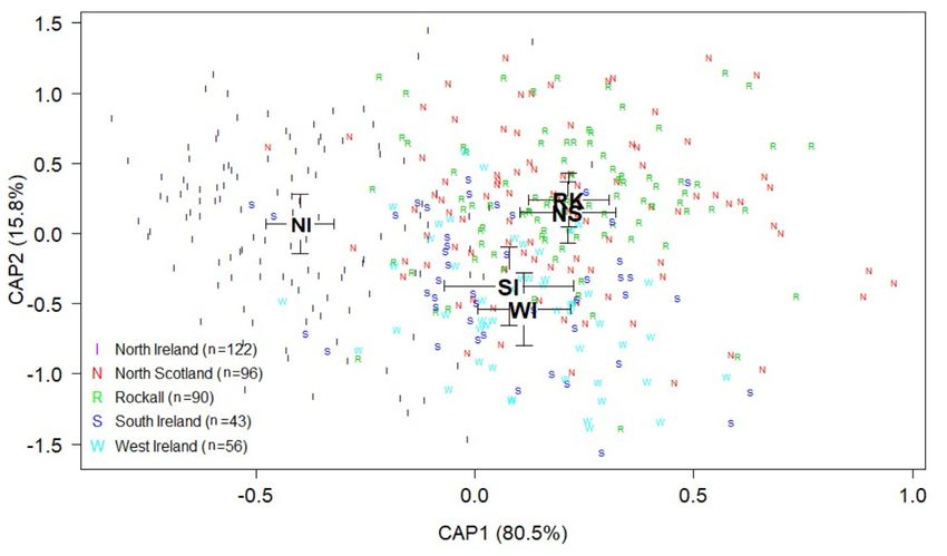
4 E. Sheerin et al.
Downloaded from https://academic.oup.com/icesjms/advance-article/doi/10.1093/icesjms/fsac039/6551738 by guest on 22 March 2022
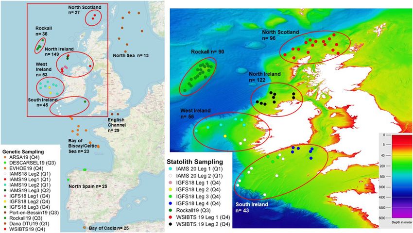
Figure 1. (Left) Sampling stations from research surveys and port sampling at Port en Bessin (see Supplementary Table S1) for L. forbesii microsatellite
and COI genetic analysis; (Right) Sampling stations for statolith shape analysis overlain on bathymetry, with sampling year and sampling quarter
information included. Red callout box and ellipses display the five sampling locations which spatially overlapped in both genetic and statolith shape
analyses (i.e. north Scotland, Rockall, north Ireland, west Ireland, and south Ireland), with sample sizes included.
PCR contained 12.5 μL of Thermo Scientific™ DreamTaq Microsatellite analysis
Green PCR Master Mix (2X), 0.5 μM of each primer, 2.5 μL A total of nine microsatellite loci was used to assess the
of DNA and 9 μL H2 O, resulting in final reaction volume nuclear genetic diversity: Lfor 2, Lfor 3, Lfor 4, Lfor 5,
of 25 μL. A negative control to ensure cross-contamination Lfor 8 (Shaw, 1997), Lfor 1 (Shaw et al., 1999), and Lfor
did not occur was incorporated to the procedure by adding 11, Lfor 12, and Lfor 16 (Emery et al., 1999). The reverse
2.5 μL of dH2 O. The PCR conditions were 94◦ C for 2 min, primer of each set was “pigtailed” using the following bases
35 cycles of 94◦ C for 40s, 50◦ C for 40s, and 72◦ C for “5”-GTTTCTT’ to enhance non-templated nucleotide ad-
90s, followed by 72◦ C for 10 min (Allcock et al., 2007). dition according to Brownstein et al. (1996). All primers
PCR products were visualised on a 1% (w/v) agarose gel were purchased in a lyophilised state from Applied Biosys-
using SYBR safe DNA Gel stain Invitrogen™ and bands of tems (Life Technologies) and eluted to 100 μM. The forward
650 bp were obtained. PCR products were cleaned using primer of each set also had a fluorescent label attached (see
Invitrogen™ PureLink™ PCR Purification Kit according to below).
the manufacturer’s instructions. Purified PCR products were The following primer sets were amplified together in three
then standardised to 12 ng/μL using a Biochrom SimpliNano multiplexes: Mix A: Lfor 5 (0.25 μM, 6-FAM™), Lfor 1
NanoDrop Spectrophotometer in accordance with the DNA (0.5 μM, PET™), Lfor 12 (0.5 μM, 6-FAM™), Lfor 16
sequencing facility specifications. Samples were prepared for (0.5 μM NED™); Mix B: Lfor 4 (0.5 μM, VIC®), Lfor 8
sequencing by adding 5 μL of each purified PCR product (0.5 μM, 6-FAM™) and Mix C: Lfor 2 (0.33 μM, 6-FAM™),
to 5 μM forward primer LCO1490 resulting in a 10 μL Lfor 3 (0.33 μM, VIC®) Lfor 11 (1 μM,6-FAM™). Each mul-
reaction volume. Samples were sent to Eurofins Genomics tiplex contained 5 μL Thermoscientific DreamTaq Hot Start
(Germany) for DNA Sequencing on an ABI 3730XL DNA Green PCR Master Mix (2X), the relevant quantities of each
Analyser. All sequences were viewed and trimmed using forward and reverse primer as listed above, 1 μL of DNA and
Sequence Scanner v2 before input into MEGA X software H2 0, resulting in a final reaction volume of 10 μL. Samples
(Molecular Evolutionary Genetics Analysis across computing were analysed in duplicate from the PCR stage to ensure re-
platforms, Kumar et al., 2016) where they were aligned peatability. A touchdown PCR was used, with the annealing
using MUltiple Sequence Comparison by Log- Expectation temperature dropping by 0.5◦ C for each cycle. This consisted
(MUSCLE) and inspected for mitochondrial diversity. Using of 94◦ C for 3 min, 16 cycles of 94◦ C for 30 s, 61◦ C for 30 s
558 bp of COI sequence, a median-joining network was con- and 72◦ C for 30 s followed by 24 cycles of 94◦ C for 30 s, 53◦ C
structed using the median algorithm of Bandelt et al. (1999), for 30 s and 72◦ C for 30 s and a final extension of 72◦ C for
implemented in the programme POPART v.1.7.1 (Leigh and 10 min. The PCR products were diluted (1:4) using nuclease-
Byrant, 2015). DnaSP v.10.01 (Librado and Rozas, 2009) free water prior to fragment analysis, and 1 μL was then
was used to estimate nucleotide diversity across the COI added to 15 μL of Hi Di Formamide with 0.2 μL of GeneS-
dataset. can™ 500 LIZ™ dye size standard.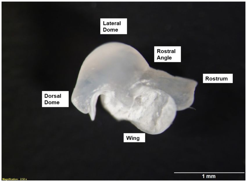
Multi-method approach shows stock structure in Loligo forbesii squid                                                                        5

Table 2. ICES WKMSCEPH maturity scale (ICES, 2010) for both males and females used in data collection on scientific surveys.

Male                                                              Female                                                       Maturity Stage

No visible maturation                                             No visible maturation                                             0
Small translucent testis. Spermatophoric complex visible          Nidamental glands translucent                                     1a
                                                                  Ovary is semi- transparent
Testis enlarged. Spermatophoric complex more developed            Nidamental glands opaque, Ovary enlarged                          2a
                                                                  Some Oocytes present
Testis at full size. Needham’s sack with partially developed      Nidamental gland large                                            2b
spermatophores

                                                                                                                                                Downloaded from https://academic.oup.com/icesjms/advance-article/doi/10.1093/icesjms/fsac039/6551738 by guest on 22 March 2022
                                                                  Ovary with some non-hydrated oocytes present
Testis at full size. Needham’s sack full of spermatophores        Nidamental gland large                                            3a
                                                                  Ovary packed with large, hydrated oocytes
Very few/no spermatophores in Needham’s sack                      Very few/no eggs in oviduct Nidamental glands degenerating        3b

   Fragment analysis was performed on an ABI Genetic Anal-                  using fine-nosed forceps. Extreme care was taken at this stage
yser 3500 and alleles were scored using GENEMAPPER                          as the wing portion of the statolith is exceptionally fragile and
Software v5 (Applied Biosystems). Any samples which gave                    prone to chipping. Both left and right statoliths were identi-
inconsistent scores between replicates or failed entirely were              fied and stored (dry) separately. In the majority of cases, only
repeated from the PCR step.                                                 the right statolith was selected for subsequent analysis, how-
                                                                            ever, if the right statolith was damaged or otherwise unusable,
Statolith shape & biological data sampling                                  the mirrored image of the left statolith, obtained using editing
                                                                            software, was used. Mirror images were justified on the ba-
All statolith samples came from the same research surveys as
                                                                            sis that studies which compared left and right statoliths have
genetics tissue samples, apart from the IAMS 2020, when only
                                                                            found that these did not differ in shape (Barcellos and Gasalla,
statoliths were sampled (no genetics samples were taken from
                                                                            2015; Green et al., 2015; Fang et al., 2018; Guo et al., 2021).
that cruise since the same area had already been sampled–
                                                                            If both statoliths displayed damage, the sample was discarded.
Figure 1; Supplementary Table S1). However, the same indi-
                                                                            From the 417 sampled individuals, 10 were rejected from the
vidual squid were not necessarily sampled for both statoliths
                                                                            analysis due to visible damage on both left and right statolith.
and genetics at each sampling station. Statoliths were collected
                                                                            The remaining 407 viable statoliths (Rockall, n = 90; north
during demersal fishery surveys (2018–2020) at a subset of the
                                                                            Scotland, n = 96; north Ireland, n = 122; west Ireland, n = 56;
locations that were sampled for genetics analysis (Figure 1,
                                                                            south Ireland, n = 43) were imaged with a stereomicroscope
Supplementary Table S1). RKS19, WSIBTS19, and IGFS18
                                                                            (Olympus SZX16, 400x) using reflected-oblique light against
are all components of the International Bottom Trawl Sur-
                                                                            a black background. Exposure time and white balance were
veys (IBTS) and used the standard Grande Overture Verti-
                                                                            calibrated in order to achieve the strongest contrast between
cale (GOV 36/47) net with mesh sizes ranging from 100 mm
                                                                            the statolith and background. The statolith from the right side
at the trawl opening to a 20 mm liner in a 25 mm cod end
                                                                            of each individual was positioned with the lateral dome facing
(Stokes et al., 2015). IAMS20 used a commercially derived
                                                                            left and anterior rostral lobe facing right, with the wing facing
otter trawl with mesh sizes of 200 mm at the trawl wings re-
                                                                            upwards (Figure 2). A 1 mm scale was included for each mag-
ducing to 100 mm in the cod-end (Reid et al., 2007). Fishing
                                                                            nification, to create a calibration measurement of the number
times during RKS19, WSIBTS19 and IGFS18 were standard-
                                                                            of pixels along the 1 mm scale that was later used for calcu-
ised to roughly 30 min at 4 knots and only occurred during
                                                                            lating the area, length, perimeter, and width of each statolith,
daylight hours. Fishing times during IAMS20 were roughly
                                                                            obtained using “ImageJ” (v1.52A) software (Schneider et al.,
1 h at 4 knots and occurred over 24 h.
                                                                            2012).
   Catches were sorted on-board and the L. forbesii portion
of the catch was put aside for biological sampling (mantle
length, weight, sex, and maturity). When feasible, biological               Data analysis
sampling was carried out for all individuals, but for stations              Microsatellite statistical analysis
with abundant squid, the subsampling procedure outlined in                  Micro-Checker v2.2.3 (Van Oosterhout et al., 2004) was used
ICES (2017) was used, i.e. a representative subsample com-                  to detect the presence of null alleles, stuttering errors or
prising >10 times the number of length classes in the sample                allelic dropout. The full dataset was analysed initially, fol-
(based on 1 cm increments in mantle length) (Gerritsen and                  lowed by subdivision of the dataset into the 10 sampling lo-
McGrath, 2007). Maturity was determined on-board research                   cations and repetition of the analysis. Genetic diversity was
vessels using the WKMSCEPH common Teuthida maturity                         assessed using GenAlEx v6.503 (Peakall and Smouse, 2006,
scale (Table 2; ICES, 2010) and individuals reaching mini-                  2012) software. Number of alleles (Na ), Observed heterozy-
mum maturity stage 2a were frozen (−20◦ C) for subsequent                   gosity (Ho ), Expected heterozygosity (He ) and Fixation in-
statolith analysis. Selecting a minimum maturity level ensured              dex (F) were calculated on both full and subdivided datasets
reliable identification of species and avoided potential arte-              and displayed in Table 1. Allelic frequency and principal co-
facts caused by ontogenic effects on statolith shape and size               ordinates analysis were also performed using GenAlEx v6.503
(Fang et al., 2018). A total of 417 individuals (males and fe-              software. Genotypic linkage disequilibrium was tested for all
males) was selected for statolith analysis across five sampling             locus pairs in each location and for each locus pair across
areas (Rockall, n = 93, north Scotland, n = 96, north Ireland,              all locations using Fisher’s Method (1000 demorisations and
n = 125, west Ireland, n = 56, south Ireland, n = 47). All                  5000 iterations) in GENEPOP v4.2. The inbreeding co-
statoliths were extracted using the methods of Clarke (1978)                efficient FIS was calculated in FSTAT v2.9.4 (Goudet, 1995) by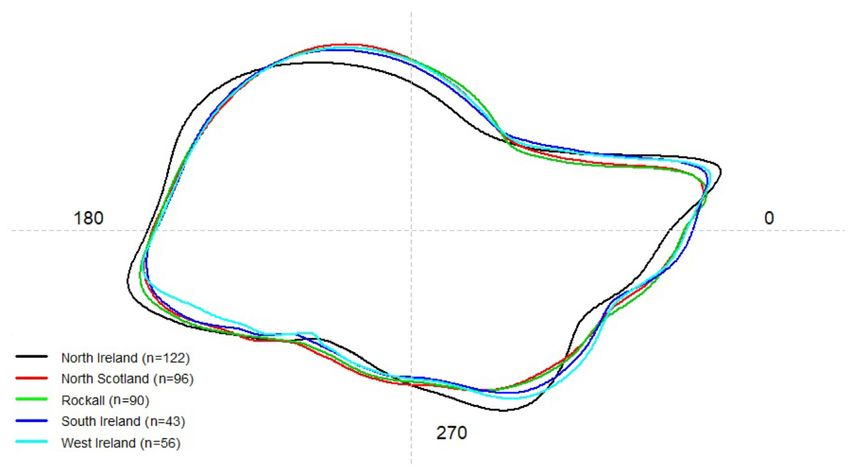
6                                                                                                                                         E. Sheerin et al.

                                                                                                                                                              Downloaded from https://academic.oup.com/icesjms/advance-article/doi/10.1093/icesjms/fsac039/6551738 by guest on 22 March 2022
Figure 2. Orientation of statolith for imaging showing labelled sub-areas of this structure. The statolith from the right side of each individual was
positioned with the lateral dome facing left and anterior rostral lobe facing right with the wing facing upwards.

randomising the alleles between all individuals in a sample                      available (i.e. excluding the English Channel location, as these
and comparing this to the observed data to determine whether                     samples were taken by means of port sampling and accurate
there were any deviations from Hardy–Weinberg Equilibrium,                       GPS co-ordinates of the catch location were not available).
using 10 000 permutations. Population structure was assessed                     Geographical distances were calculated based on the distances
using STRUCTURE v2.3.4 software (Pritchard et al., 2000),                        between sampling stations. GPS co-ordinates from a total of
which uses Bayesian clustering methods on allele frequencies                     57 sampling stations were entered into GenAlEx to produce
to find the most likely number of populations (K) present                        a tri matrix table of logged geographical distances between
within the dataset. This was performed on both the full and                      each station. Linearised FST values were then plotted against
subdivided (by sampling location) dataset. The range of K was                    the logged geographical distance.
set between 1 and 5, with each model consisting of 5 runs.
Each run contained a burn-in period of 200 000 with 500 000                      Statolith shape and biological data analysis
MCMC reps. An admixture model was used with the corre-                           Shape analysis was completed using the ShapeR package (Li-
lated allele frequencies parameter selected and the data were                    bungan and Pálsson, 2015) in R (R Core Team, 2019). The
run both with and without the LOCPRIOR function which is                         first stage of this process was to extract the outlines for all
used to infer prior location information of the samples. The                     statoliths and write them into the ShapeR package. This oper-
programme STRUCTURE Harvester (Earl and Von Holdt,                               ation converts images into grey-scale and picks out the out-
2012) was used to implement the Evanno method (Evanno                            line using a pre-set threshold pixel value. From this, shape
et al., 2005), in which the L(K) and (K) values were used to                    coefficients for each statolith are produced using the discrete
identify the most likely K value. Evanno et al. (2005) showed                    wavelet-transform method, which decomposes images into a
that the use of (K) does not allow the assessment of K = 1                      number of “wavelets” that have an amplitude that begins at
as a potential solution so that assessment of the L(K) graph                     zero, increases, and then decreases back to zero and is irreg-
is the most appropriate analysis when K = 1. POPHELPER                           ular in shape and compactly supported (Graps, 1995). Due
R package (Francis, 2017) was used to graphically illustrate                     to their irregular shape, wavelets are ideal for analysing com-
the results obtained using STRUCTURE software. To further                        plex shapes with many discontinuities or sharp edges, such as
examine the presence of genetic structure, a principal coordi-                   statoliths (Fang et al., 2018) and are better suited to this task
nates analysis (PCoA) in GenAIex v.6.5b (Peakall and Smouse,                     than Fourier-transform shape analysis which does not approx-
2006) was used as a multivariate approach to supplement the                      imate sharp edges as accurately (Graps, 1995; Libungan et al.,
STRUCTURE analysis.                                                              2015b). The ShapeR package uses this technique to produce
   Genetic differentiation was evaluated with the software FS-                   a total of 64 wavelet coefficients (five wavelet levels) which
TAT v2.9.4 (Goudet, 1995) using randomisation of genotypes.                      describe the shape for each statolith (Libungan and Pálsson,
A pairwise test of FST values was generated under 1000 per-                      2015; Libungan et al., 2015b). To take into account any allo-
mutations and Bonferroni correction for multiple tests was ap-                   metric relationships with mantle length, wavelet coefficients
plied. A Mantel test was performed in GenAlEx v6.503 soft-                       which show interaction (p < 0.05) with length, are omit-
ware (Peakall and Smouse, 2006, 2012) to test for isolation                      ted automatically and the remaining coefficients are standard-
by distance in all samples for which geographic distance was                     ised for length. Variation in statolith shape was then visually
Multi-method approach shows stock structure in Loligo forbesii squid 7
represented by plotting mean statolith shape for all five groups allele dropout resulted in scoring errors. There was, however,
(i.e. sampling locations) using length-standardised wavelet co- some evidence of null alleles (based on the combined prob-
efficients. The matrix of wavelet standardised coefficients was ability for homozygote frequencies at all allele size classes,
analysed amongst groups using canonical analysis of princi- p < 0.001) in the following three loci: Lfor 8, Lfor 12, and
pal coordinates (CAP) based on Euclidean dissimilarity indices Lfor 16. Analysis of the subdivided dataset by sampling lo-
(Libungan, 2015). Each individual statolith was ordinated us- cation, showed that none of the loci consistently produced
ing CAP, allowing distances between groups of statoliths to significant levels of null alleles across all locations. Statistical
be examined. A cluster plot was used to visually represent the analysis was completed with and without the worst affected
grouping of CAP results in two dimensions. Following this, the loci for null alleles, Lfor 8 and Lfor 12, which were found to
Downloaded from https://academic.oup.com/icesjms/advance-article/doi/10.1093/icesjms/fsac039/6551738 by guest on 22 March 2022
partitioning of variation among groups based on their canon- have a negligible impact on the overall dataset. Hence the re-
ical score was tested with an ANOVA-like permutation test sults for the full dataset including all nine loci are presented
(permANOVA) using the Vegan package for R (Oksanen et below, unless otherwise indicated.
al., 2013). The permANOVA was then repeated for each pair Genetic diversity indices are displayed in Table 1 for nine
of sampling locations in order to investigate pairwise associ- microsatellite loci at 10 sampling locations (n = 425 individ-
ations in statolith shape. To protect against the influence of uals). The sampling locations exhibited high mean values for
type one errors, the p-value accepted for significance in this the Na index (numbers of alleles) ranging from 11.2 (North
pairwise analysis was adjusted using a Bonferroni correction. Sea) to 19.9 (north Ireland), averaging 14.7 overall. Allelic
Data from biological sampling (dorsal mantle length richness (Ar ) was also high, ranging from 9.3 to 10. Observed
(DML), sex and maturity) were also compared between loca- and expected heterozygosities per sampling location were very
tions for the same individuals which had been analysed using similar overall, respectively ranging from 0.771–0.838 (aver-
statoliths (n = 407). Sex and maturity ratios were compared age 0.802) to 0.852–0.878 (average 0.866), indicating high
between all locations using a chi-square test. Prior to analysis, diversity within all locations.
maturity information was converted to a binary (0, 1) scale None of the inbreeding co-efficient (FIS ) values obtained
with individuals of maturity 2a being designated 0 (“matur- from the 10 sampling locations deviated from Hardy–
ing”) and those of 2b and 3a being designated 1 (“mature”). Weinberg Equilibrium at p < 0.0006 following Bonferroni
DML data were analysed separately for each sex, comparing correction for multiple comparisons (Table 1). Significant link-
between locations (male: n = 191, female: n = 216) after age disequilibrium was detected at only one pair of loci (north
first being tested for normality and homoscedasticity using Ireland Lfor 5 x Lfor 2) at p < 0.0001 following Bonferroni
Kolmogorov–Smirnov and Levene’s tests. Where transfor- correction. No significant linkage disequilibrium was detected
mations failed to normalise the data, non-parametric tests for any locus pair across all populations at p < 0.0001 after
(Kruskal–Wallis) were used to analyse between-location vari- Bonferroni correction.
ation in DML of both males and females, followed by pairwise
comparisons using a Dunn–Bonferroni post-hoc test.
To help interpret L. forbesii statolith shape comparisons be- Genetic structure
tween locations, a small sample of Loligo vulgaris was also Pairwise FST values between sampling locations were very low,
analysed to provide context, i.e. to place the shape variabil- both with (−0.009 to 0.005) and without (−0.007 to 0.008)
ity across L. forbesii samples into perspective when compared the worst affected loci for null alleles (Lfor 8 and Lfor 12)
with a closely related species. For this, a sample of L. vulgaris (Table 3). This indicates that the presence of null alleles in
(n = 20) was obtained during the IGFS18 in the Celtic Sea loci Lfor 8 and Lfor 12 did not impact on the overall result
(ICES Division 7g) from 7th to 10th December 2018. This was that genetic structure is lacking between sampling locations.
analysed following the same statolith processing and statisti- When all nine loci were included, the pairwise FST resulted in
cal analysis steps as before and was compared with L. forbesii one significant pairwise test (Rockall versus north Ireland) at
data across all locations. p < 0.001 after Bonferroni correction for multiple tests was
applied (data not shown), but when Lfor 8 and Lfor 12 were
removed from the data, none of the sampling locations were
Results significantly differentiated from one another once Bonferroni
Mitochondrial DNA (COI) Analysis correction had been applied (Table 3). Despite not meeting
A total of eight haplotypes were found in this study. The the threshold for statistical significance, seven comparisons
most common haplotype, H1, occurred throughout the sam- out of 45 were “significant” at p < 0.05 prior to Bonferroni
pled area, with the remaining seven haplotypes occurring in correction, six of which involved Rockall (Table 3). These six
relatively few samples (Supplementary Figure S1). Across the locations were: north Scotland, north Ireland, west Ireland,
558 bp of sequence, 547 sites were monomorphic, 11 poly- English Channel, north Spain and Cadiz, with pairwise FST
morphic (including a total of 11 mutations), seven sites in- values versus Rockall ranging from 0.003 to 0.008 (Table 3).
cluded singletons and four sites were parsimony-informative. The remaining comparison showing p < 0.05 prior to Bonfer-
Additional metrics included an overall nucleotide diversity, roni correction was west Ireland versus Cadiz (pairwise FST of
Pi = 0.00621 ± 0.00142 and gene or haplotype diversity, 0.004–Table 3).
Hd = 1.000 ± 0.063. The STRUCTURE results showed that there was no ev-
idence of genetic partitioning in the dataset and the popu-
lation displays high levels of admixture—see bar plots for
Microsatellite analysis K = 2, K = 3, K = 4, and K = 5 (Figure 3a). STRUC-
Most samples were successfully genotyped in duplicate with TURE analysis indicated a population of K = 1, supported
success rates ranging from 88% in Lfor 8 to 100% in both by the L(K) graph, which showed the most likely value to be
Lfor 1 and Lfor 3. There was no evidence that stuttering or K = 1, based on posterior probabilities (Figure 3b). The PCoA8 E. Sheerin et al.
Table 3. Results of pairwise FST values between sampling locations using seven microsatellite loci (i.e. omitting loci Lfor 8 and Lfor 12, which were affected
by null alleles). Underlined values indicate statistical significance at p < 0.05 which became non-significant after Bonferroni correction was applied (cut-off
for statistical significance at p < 0.001). Sample location abbreviations are listed in full in Table 1.
Sample location NS RK NI WI SI NSea ECh NSp Cad BB
NS –
RK 0.003 –
NI − 0.001 0.005 –
WI − 0.004 0.004 0.001 –
SI − 0.001 0.003 − 0.001 -0.002 –
Downloaded from https://academic.oup.com/icesjms/advance-article/doi/10.1093/icesjms/fsac039/6551738 by guest on 22 March 2022
NSea − 0.005 − 0.002 − 0.004 0.000 − 0.006 –
ECh − 0.003 0.007 0.001 0.000 − 0.001 − 0.002 –
NSp − 0.002 0.003 − 0.001 0.000 − 0.003 − 0.005 -0.003 –
Cad − 0.002 0.008 0.000 0.004 0.004 0.002 − 0.003 − 0.006 –
BB − 0.004 0.003 − 0.004 − 0.003 − 0.004 − 0.003 − 0.005 − 0.005 − 0.007 –
Figure 3. (a) STRUCTURE assignment of individuals across all subdivided sample sites using LOCPRIOR function for the following values of K (K = 2),
(K = 3), (K = 4), and (K = 5) displayed via the POPHELPER package. The numbers on the x-axis refer to the sample locations listed in Table 1. (b) Mean
likelihood L(K) ± standard deviation per K value produced by STRUCTURE Harvester and visualised in POPHELPER indicating that 1 is the true value of K.
(Supplementary Figure S2) was also used to assess whether females (H = 36.669, 4 df, n = 216, p > 0.05). Pairwise com-
any genetic patterns were present and this showed no evi- parisons using a Dunn–Bonferroni post-hoc test conducted on
dence of clustering by sampling locations. Mantel’s test re- male DML data (Table 4 with significance cut-off adjusted for
vealed significant Isolation By Distance (IBD), with a weak multiple comparisons) showed significant differences in DML
negative trend and a very low fit (R2 = 0.0059, p < 0.05, between south Ireland (median DML 170 mm) and north Ire-
Supplementary Figure S3). land (median DML 220 mm), south Ireland and west Ire-
land (median DML 275 mm), south Ireland and Rockall (me-
Biological data dian DML 290 mm), and between north Scotland (median
DML 190 mm) and north Ireland, west Ireland, and Rockall.
No significant between-location variation in sex ratio was
Thus, the largest median size was seen in males from Rock-
found (χ 2 = 7.220, 4 df, n = 407, p > 0.05). However, matu-
all, followed by west Ireland, north Ireland, north Scotland,
rity ratios (maturing/mature) varied significantly between lo-
and south Ireland, however, the data distributions were highly
cations with Rockall containing a higher frequency of “matur-
overlapping and multi-modal (Figure 4).
ing” individuals (stage 2a) and all other locations containing
more “mature” individuals (stages 2b and 3a) (χ 2 = 72.618,
4 df, n = 407, p < 0.05, Figure 4). The K-S test statistic in- Statolith shape, CAP ordination, and mean plots
dicated that neither male (K-S D = 0.133, p < 0.05) nor The statolith outline was reconstructed with > 98.5% ac-
female (K-S D = 0.115, p < 0.05) DML data were nor- curacy using five wavelet levels (Supplementary Figure S4a).
mally distributed and a Levene’s test revealed that the as- Visual representation of mean statolith shape under discrete
sumption of homogeneity of variance was met only in males wavelet reconstruction showed observable differences be-
(F = 1.364, n = 191, 4 df, p > 0.05) but not in females tween all locations along the wing, rostral angle, lateral dome
(F = 4.994, n = 216, 4 df, p < 0.05), despite attempts at and dorsal dome regions of the statolith (Figure 5). An in-
transformation, hence a Kruskal–Wallis test was used on un- traclass correlation (ICC) plot displaying the proportion of
transformed DML data of both sexes. This showed signifi- variance among groups (i.e. locations) in wavelet coefficients
cant differences in DML between sampling locations in males confirmed that most of the variation among groups can be at-
(H = 9.231, 4 df, n = 191, p < 0.05, Figure 4) but not in tributed to angles 140–180◦ , 190–230◦ (lateral/dorsal dome),Multi-method approach shows stock structure in Loligo forbesii squid 9
Downloaded from https://academic.oup.com/icesjms/advance-article/doi/10.1093/icesjms/fsac039/6551738 by guest on 22 March 2022
Figure 4. Histograms of dorsal mantle length in male Loligo forbesii. The magnitude of the x- and y-axis is the same in each location to aid comparison.
Arrows indicate median length for each location.
Table 4. Dunn–Bonferroni pairwise comparisons between locations based on Kruskal–Wallis comparison of male DML in Loligo forbesii. SI = south Ireland,
NS = north Scotland, NI = north Ireland, WI = west Ireland, RK = Rockall. Values in bold/underline are statistically significant.
Comparison Median DML (mm) Range (mm) Test Statistic Std. Test Statistic Adj. Sig.
S Ireland = N Scotland SI: 170 SI: 410 15.339 1.083 1.000
NS: 190 NS: 260
S Ireland < N Ireland SI: 170 SI: 410 − 51.376 − 3.810 0.001
NI: 220 NI: 300
S Ireland < W Ireland SI: 170 SI: 410 − 64.708 − 3.599 0.003
WI: 275 WI: 350
S Ireland < Rockall SI: 170 SI: 410 65.906 4.655 0.000
RK: 290 RK: 220
N Scotland < N Ireland NS: 190 NS: 260 − 36.037 − 3.332 0.009
NI: 220 NI: 300
N Scotland < W Ireland NS: 190 NS: 260 − 49.369 − 3.071 0.021
WI: 275 WI: 350
N Scotland < Rockall NS: 190 NS: 260 − 50.567 − 4.343 0.000
RK: 290 RK: 220
N Ireland = W Ireland NI: 220 NI: 300 13.332 0.861 1.000
WI: 275 WI: 350
N Ireland = Rockall NI: 220 NI: 300 14.530 1.343 1.000
RK: 290 RK: 220
W Ireland = Rockall WI: 275 WI: 350 1.198 0.075 1.000
RK: 290 RK: 220
and 310–360◦ (wing/rostrum) (Supplementary Figure S4b). second axis (CAP2) explained 15.8% of variation. Canonical
North Ireland was strongly distinguished from other locations values for both Rockall and north Scotland oriented to the
in overall mean statolith shape, especially in the dorsal and upper right and centre of the plot while south and west Ire-
lateral dome and wing section (Figure 5). Highest perimeter- land values were situated in the centre and lower right of the
area ratios, which correspond to shape complexity in the sta- plot. North Ireland, on the centre left, was found to be most
tolith (measured in two dimensions) were observed in south distant from the other locations. Squid size did not affect this
Ireland, whereas these ratios were lower in north Scotland, ordination since there was no correlation between DML and
north Ireland, and Rockall (Supplementary Table S2). Figure 6 CAP1 score (Supplementary Figure S5). With the exception of
displays canonical principle coordinates (CAP) scores based Rockall versus north Scotland, comparisons of scores between
on Euclidean dissimilarity indices, including mean scores per pairs of locations were all significantly different from one an-
location ± standard error. The first discriminating axis (CAP1) other by permANOVA (F = 27.423, 4 df, adjusted p-value
explained 80.5% of variation among locations while the cut-off = 0.005, n = 407, Table 5).10 E. Sheerin et al.
Downloaded from https://academic.oup.com/icesjms/advance-article/doi/10.1093/icesjms/fsac039/6551738 by guest on 22 March 2022
Figure 5. Mean statolith shape of L. forbesii (males and females) in north Ireland (black), north Scotland (red), Rockall (green), south Ireland (blue) and
west Ireland (cyan) under discrete wavelet reconstruction. The numbers show angle in degrees (◦ ) based on polar coordinates where the centroid of the
statolith is the center point of the polar coordinates.
Figure 6. Canonical scores on discriminating axes CAP1 and CAP2 for each L. forbesii location: north Ireland (I, black), north Scotland (N, red), Rockall (R,
green), south Ireland (S, blue) and west Ireland (W, cyan). Large black letters represent the mean canonical value (± standard error) for each location and
smaller coloured letters represent individual squid (SI = south Ireland, NS = north Scotland, NI = north Ireland, WI = west Ireland, RK = Rockall).
Table 5. PermANOVA results of CAP ordination of wavelet coefficients between all 10 pairs of sampling locations. Significance between each pair of areas
was analysed using a Bonferroni–adjusted p-value cut-off of 0.005. All comparisons were statistically significant except where indicated (NS).
Comparison df F P
S Ireland—N Scotland 1 7.34 < 0.001
S Ireland—N Ireland 1 29.04 < 0.001
S Ireland—W Ireland 1 2.94 0.004
S Ireland—Rockall 1 9.82 < 0.001
N Scotland—N Ireland 1 57.79 < 0.001
N Scotland—W Ireland 1 11.37 < 0.001
N Scotland—Rockall 1 2.11 0.040 (NS)
N Ireland—W Ireland 1 40.58 < 0.001
N Ireland—Rockall 1 60.97 < 0.001
W Ireland—Rockall 1 14.08 < 0.001
The shapes of L. forbesii and L. vulgaris statoliths were between L. vulgaris and L. forbesii shows that canonical
also analysed using CAP ordination scores. This time, CAP1 scores for L. forbesii from all locations oriented much the
explained 14.9% of the disparity between species/locations same as in Figure 6 and L. vulgaris scores clustered be-
while CAP2 explained 76.6% of this variation. Differentiation tween the L. forbesii scores at Rockall/north Scotland andMulti-method approach shows stock structure in Loligo forbesii squid 11
south/west Ireland but distant from the L. forbesii from north Rockall and two shelf locations—west of Scotland (but only in
Ireland (Supplementary Figure S6). A permANOVA showed one of two years sampled) and English Channel. Other differ-
that the shape coefficients in the two species were statistically ences in that study, i.e. between Rockall–north west Spain and
different from one another (F = 23.408, 5 df, p < 0.05). Rockall–west of Scotland (in the second of the sampled years),
were no longer significant after Bonferroni correction was ap-
plied (Shaw et al., 1999). Shaw et al. (1999) suggested the iso-
Discussion lation arose due to deep water and oceanography which could
The genetic markers examined in the present study showed no present a potential barrier to isolate offshore populations like
significant evidence of sub-structure in Loligo forbesii from 10 Rockall from the shelf population. Our results contrast with
Downloaded from https://academic.oup.com/icesjms/advance-article/doi/10.1093/icesjms/fsac039/6551738 by guest on 22 March 2022
locations across the NE Atlantic but some non-significant evi- this: we found no statistically significant evidence of genetic
dence of structure was observed at Rockall. By contrast, good sub-structure between similar sampling locations, including
spatial differentiation was seen in the statolith shape markers, an additional six locations which were not sampled before; the
highlighting the fact that ecologically separated groups can be North Sea, the northern Bay of Biscay, north, west and south
identified in this species. New insight from both genetic and Ireland and south Spain. It should be noted that there was
ecological markers allows us to re-interpret the stock struc- not complete overlap between the markers used in both cases:
ture of L. forbesii, both in locations previously shown to be of the nine microsatellite markers used in the present study,
isolated i.e. Rockall, as well as in locations previously shown only five markers overlapped directly with Shaw et al. (1999)
to be homogeneous i.e. continental shelf areas, especially Ma- study. So although we had two additional markers in total,
lin Shelf in the north of Ireland. we also had four different markers in comparison to Shaw
Discussing the genetic marker results first, very low levels of et al. (1999). That said, the loci which were most variable
diversity were observed in the mitochondrial DNA (mtDNA) in the past regarding Rockall (Lfor 1 and Lfor3; Shaw et al.,
COI gene in L. forbesii with only 8/425 sequences show- 1999) were included in the present study. Null alleles (caused
ing haplotypic variation. The majority of the samples con- by a mismatch between the primer and the target sequence re-
tained the same haplotype, H1, which occurred throughout sulting in alleles which fail to amplify) are known to inflate
the dataset and formed the centre of a network with low lev- FST values (Chapuis and Estoup, 2007). Previous studies have
els of sequence diversity. Other genes should be examined in shown that null alleles are common in mollusc populations
future studies, given the low variability seen in the COI gene, with large effective population sizes (Li et al., 2003; Kaukinen
which is useful for DNA barcoding studies (Gebhardt and et al., 2004; Astanei et al., 2005; Ramos et al., 2018). In the
Knebelsberger, 2015; Maggioni et al., 2020), but relatively un- present study, prior to removal of loci affected by null alleles,
informative for studies such as this, where a faster evolving there was one comparison involving Rockall versus northern
section of the mtDNA such as the control region may pro- Ireland which was significant at p < 0.001 after Bonferroni
vide additional data. Interestingly, while other loliginids also correction. But once loci which were shown to be most af-
showed low mtDNA variation (Aoki et al., 2008; Ibáñez et fected by null alleles (Lfor 8 and Lfor 12) had been removed,
al., 2012), analysis of 55 Loligo vulgaris samples from Galicia and once a Bonferroni correction had been applied, no sig-
in north west Spain using this gene resulted in 35 haplotypes, nificant differences remained between Rockall and the other
indicating high COI diversity in this species at that location sampling locations. Further analysis to detect genetic structure
(Garcia-Mayoral et al., 2020). using STRUCTURE analysis and Principal Coordinate Analy-
High genetic diversity was observed in the microsatellite sis (PCoA) also showed no differentiation. Sampling of squid
markers at nine loci in the present study (mean Ho = 0.802, is opportunistic and is dependent on national groundfish sur-
He = 0.866 in L. forbesii at all locations) and each microsatel- vey dates but this should not have impacted on results. Sam-
lite locus was highly polymorphic with 11.2–19.9 alleles per ples were taken in 2019 at all locations, apart from south Ire-
locus, depending on the location. These values are similar to land (2018), and all locations contained genetic samples taken
previous observations in L. forbesii by Shaw et al. (1999) and in Q4 apart from Rockall, north Spain and English Channel
they also fall within the range of values reported in Todarop- (sampled in Q3) and North Sea (Q1) (details of sampling quar-
sis eblanae (Ho = 0.83–0.93, He = 0.85–0.93, alleles per lo- ters and years are given in Supplementary Table S1).
cus 9.6–27, Dillane et al., 2005), but are a bit higher than Se- Unlike genetic markers, differences in L. forbesii statolith
pioteuthis australis (Ho = 0.519–0.585, He = 0.735–0.777, shape were apparent between four out of five locations anal-
alleles per locus 10.71–12, Smith et al., 2015), and Dosidi- ysed by statolith shape markers. The north Ireland statoliths
cus gigas (Ho = 0.657–0.759 He = 0.815–0.833, alleles per were highly distinct from the rest, but other locations also
locus not provided, Sanchez et al., 2020). Microsatellites re- had pairwise differences (with the exception of Rockall versus
vealed no statistically significant population sub-structure be- north Scotland). What this suggests is that a) statolith shape is
tween sample locations in the present study, indicating high highly sensitive to local conditions and b) L. forbesii forms dis-
gene flow in L. forbesii across the sampled range. Neverthe- tinguishable groups (based on statolith shape statistics), main-
less, six of the seven comparisons that were significantly dif- taining these for long enough for local conditions to affect the
ferent prior to Bonferroni correction involved Rockall versus shape of the statolith. Thus, statolith shape is an “ecological
various shelf locations. Given this non-random pattern, the marker” in L. forbesii which can indicate a spatial structure.
fact that the Bonferroni correction is known to be conserva- Rockall, north Scotland and north Ireland were all sampled
tive with increased Type II error (Narum, 2006), and previous for statoliths in the same year (2019, Q3/Q4) so temporal
results showing subtle genetic structure at Rockall, this pat- sampling variation cannot explain differences between north
tern is interesting and should be considered. Ireland and these others (Rockall in Q3 was sampled only 6–8
Shaw et al. (1999) examined seven microsatellite markers weeks apart from north Scotland and north Ireland in Q4 in
in L. forbesii, revealing significant pairwise FST differences be- 2019). Furthermore, the remaining locations, west and south
tween samples from Rockall and Faroe Banks, and between Ireland, were sampled in Q4 (2018) plus Q1 of 2020, i.e. theYou can also read