399 Modeling extreme events: time-varying extreme tail shape - SVERIGES RIKSBANK WORKING PAPER SERIES - Bernd Schwaab
←
→
Page content transcription
If your browser does not render page correctly, please read the page content below
399
 SVERIGES RIKSBANK
 WORKING PAPER SERIES

Modeling extreme events:
time-varying extreme tail shape

Bernd Schwaab, Xin Zhang and André Lucas
December 2020
WORKING PAPERS ARE OBTAINABLE FROM

                                  www.riksbank.se/en/research
                            Sveriges Riksbank • SE-103 37 Stockholm
                                 Fax international: +46 8 21 05 31
                             Telephone international: +46 8 787 00 00

                     The Working Paper series presents reports on matters in
                    the sphere of activities of the Riksbank that are considered
                                to be of interest to a wider public.
                   The papers are to be regarded as reports on ongoing studies
                      and the authors will be pleased to receive comments.

The opinions expressed in this article are the sole responsibility of the author(s) and should not be
                   interpreted as reflecting the views of Sveriges Riksbank.
Modeling extreme events:
time-varying extreme tail shape∗
Bernd Schwaab,(a) Xin Zhang,(b) André Lucas (c)
(a)
European Central Bank, Financial Research
(b)
Sveriges Riksbank, Research Division
(c)
Vrije Universiteit Amsterdam and Tinbergen Institute
Sveriges Riksbank Working Paper Series
No. 399
Abstract
We propose a dynamic semi-parametric framework to study time variation in tail pa-
rameters. The framework builds on the Generalized Pareto Distribution (GPD) for
modeling peaks over thresholds as in Extreme Value Theory, but casts the model in
a conditional framework to allow for time-variation in the tail shape parameters. The
score-driven updates used improve the expected Kullback-Leibler divergence between
the model and the true data generating process on every step even if the GPD only fits
approximately and the model is mis-specified, as will be the case in any finite sample.
This is confirmed in simulations. Using the model, we find that Eurosystem sovereign
bond purchases during the euro area sovereign debt crisis had a beneficial impact on
extreme upper tail quantiles, leaning against the risk of extremely adverse market out-
comes while active.
Keywords: dynamic tail risk, observation-driven models, extreme value theory, Eu-
ropean Central Bank (ECB), Securities Markets Programme (SMP).
JEL classification: C22, G11.
∗
Author information: André Lucas, VU University Amsterdam, De Boelelaan 1105, 1081 HV Amsterdam,
The Netherlands, Email: a.lucas@vu.nl. Bernd Schwaab, Financial Research, European Central Bank,
Sonnemannstrasse 22, 60314 Frankfurt, Germany, email: bernd.schwaab@ecb.int. Xin Zhang, Research
Division, Sveriges Riksbank, SE 103 37 Stockholm, Sweden, email: xin.zhang@riksbank.se. An earlier version
of this paper was circulated as “Tail risk in government bond markets and ECB unconventional policies.”
Schwaab thanks ECB DG-M for comments and access to high-frequency data on SMP bond purchases. The
views expressed in this paper are those of the author and they do not necessarily reflect the views or policies
of the European Central Bank or Sveriges Riksbank.1 Introduction
This paper proposes a novel semi-parametric framework to study time variation in tail fatness
for long univariate time series, applied to high-frequency government bond returns during
times of unconventional central bank policies. The new method builds on ideas from Ex-
treme Value Theory (EVT) by using a conditional Generalized Pareto Distribution (GPD)
to approximate the tail beyond a given threshold, and endowing this conditional GPD dis-
tribution with time-varying parameters. The GPD is an appropriate tail approximation for
most heavy-tailed densities used in econometrics and actuarial sciences; see, for example,
Embrechts et al. (1997), Coles (2001), and McNeil et al. (2010, Chapter 7). As a result, the
GPD plays a central role in the study of extremes, comparable to the role the normal distri-
bution plays when studying observations in the center of the distribution. Our framework
allows us to study the time-variation in tail parameters associated with time series observa-
tions from a wide class of heavy-tailed distributions; see Rocco (2014) for a recent survey
of EVT methods in finance. We discuss the handling of non-tail time series observations,
inference on deterministic and time-varying parameters, and ways to relate time-varying
parameters to observed covariates. In this context we also study the effect of time-varying
pre-filtering methods possibly applied to the data before the dynamic GPD model is fitted.
In our model, the time-varying tail shape and tail scale parameters of the GPD are driven
by the score of the local (time t) objective function; see e.g. Creal et al. (2013) and Harvey
(2013). In this approach, the time-varying parameters are perfectly predictable one step
ahead. This makes the model observation-driven in the terminology of Cox (1981). The
log-likelihood is known in closed form, facilitating parameter estimation and inference via
standard maximum likelihood methods. Simulation evidence reveals that our model and
estimation approach is able to recover the time-varying tail shape and tail scale parameters
sufficiently accurately, as well as EVT-based market risk measures such as Value-at-Risk
(VaR) and Expected Shortfall (ES) at high confidence levels (say, 99%). This is the case
even if the model is misspecified or the GPD approximation is not exact. The latter is
particularly important in our finite sample setting, where the limiting result of the GPD can
1only hold approximately given the choice of a finite exceedance threshold in any particular
sample.
We apply our modeling framework to study the location, scale, and upper tail impact of
bond purchases undertaken by the Eurosystem – the European Central Bank (ECB) and its
17 national central banks at the time – during the euro area sovereign debt crisis between
2010 and 2012. We focus on bond purchases within the Eurosystem’s Securities Markets
Programme (SMP), which targeted sovereign bonds of five euro area countries: Greece,
Ireland, Italy, Portugal, and Spain. Based on high-frequency data for five-year benchmark
bonds, and explicitly accounting for time-variation in fat tails, we find that purchases lowered
the conditional location (mean) of future bond yields by up to -2.9 basis points (bps) per e1
bn of purchases. The impact estimates for the two largest SMP countries, Italy and Spain,
are -1.5 bps and -2.6 bps per e1 bn of purchases, respectively. These impact estimates are
marginally smaller in absolute value than earlier estimates based on different methodologies;
see Eser and Schwaab (2016), Ghysels et al. (2017), and Pooter et al. (2018).
In addition, we find that SMP purchases had a beneficial impact on the extreme upper
tail quantiles of yield changes. This suggests that central bank bond purchases lean against
the risk of extremely adverse market outcomes while they are active. The beneficial impact is
mostly explained by moving the center of the predictive distribution to the left and narrowing
it. Beneficial secondary effects come about via the SMP’s effect on tail shape and tail scale
for large economies such as Spain and Italy. The impact of purchases on tail quantiles is
larger than their impact on the conditional location (mean). We estimate that the 97.5%
VaR was reduced by 3.8, 6.0, 5.9, 2.1, and 6.9 bps per e1 bn Eurosystem intervention
in Spanish, Greek, Irish, Italian, and Portuguese five-year benchmark bonds, respectively.
The impact grows with the extremeness of the VaR. We estimate that the 99.5% VaR was
reduced, respectively, by 5.1, 10.1, 12.5, 2.9, and 15.4 bps per e1 bn of Eurosystem purchases
in the above bonds. The tail impact of the SMP purchases is economically relevant because
extreme tail risks alone can force dealer banks and market makers to retreat from supplying
liquidity to important segments of the sovereign bond market, particularly when their own
VaR constraints are binding; see Vayanos and Vila (2009) and Adrian and Shin (2014). In
2turn, malfunctioning sovereign bond markets can impair the transmission of the common
monetary policy to all parts of the euro area. Pelizzon et al. (2013, 2016) provide evidence
that market makers withdrew from trading Italian debt securities in 2011.
Our paper is related to at least two strands of literature: one on modeling time-variation
in tail parameters and one on assessing the effectiveness of central bank unconventional
monetary policy measures. Regarding the first, several papers propose methodology to study
time variation in the tail index. Davidson and Smith (1990), Coles (2001, Chapter 5.3),
and Wang and Tsai (2009), among others, also index the GPD tail parameters with time
subscripts and equip them with a parameterized structure. Our approach is different in that
their “tail index regression” approach requires conditioning variables that explain (all of) the
tail variation. Such variables are not always available. By contrast, our “filtering approach”
does not require such conditioning variables, and is arguably better suited for the real-time
monitoring of extreme risks. Second, Quintos et al. (2001), Einmahl et al. (2016), Hoga
(2017), and Lin and Kao (2018) derive formal tests for a structural break in the tail index.
A number of subsequent studies applied such tests to financial time series data. Werner
and Upper (2004) identify a break in the tail behavior of high-frequency German Bund
future returns. Galbraith and Zernov (2004) argues that certain regulatory changes in U.S.
equity markets have altered the tail index dynamics of equities returns, and Wagner (2005)
demonstrates that changes in government bond yields appear to exhibit time-variation in
the tail shape for both the U.S. and the euro area. de Haan and Zhou (2020) propose a
non-parametric approach to estimating the extreme value index locally. Our paper adds
to this strand of conditional EVT literature by proposing a model that allows us to study
both the tail shape and tail scale dynamics directly in a semi-parametric way. Explanatory
covariates can be included in the dynamics of both parameters, and likelihood ratio tests
are available to test economically relevant hypotheses. Finally, unlike Patton et al. (2019),
our tail VaR and ES dynamics explicitly account for fat tail shape beyond a threshold as
emerging from EVT. The dynamics based on the score for the GPD contain weights for
extreme observations. Such weights are absent in the elicitable score functions of Patton
et al.. The resulting dynamics in our model are, as a result, more robust, particularly for
3the ES.
A second strand of literature assesses the impact of central bank asset purchases on bond
yields and yield volatility. For example, Ghysels et al. (2017) study the yield impact of SMP
bond purchases by considering bond yields and purchases at 15-minute intervals. In this way
they mitigate a bias that unobserved factors could have introduced. The authors estimate
that SMP interventions had an impact on the conditional mean of 10-year maturity bonds
of between -0.2 and -4.2 bps per e1 bn of purchases. Eser and Schwaab (2016) study yield
impact based on daily data. In their framework, identification is based on a panel model
that exploits the cross-sectional dimension of the data. They find that, in addition to large
announcement effects, purchases of 1/1000 of the respective outstanding debt had an impact
of approximately -3 bps at the five-year maturity. Pooter et al. (2018) use the published
weekly data of aggregate SMP purchases to test for an impact on country-specific sovereign
bond liquidity premia. The authors find an average impact of -2.3 bps for purchases of
1/1000 of the outstanding debt. Our paper adds to the growing literature on assessing the
effectiveness of central bank asset purchase programs by developing methodology for the
extreme tail of the distribution.
Whereas de Haan and Zhou (2020) take a non-parametric perspective, the methodologi-
cal part of this paper is closest to Massacci (2017), who also proposes a dynamic parametric
model for the GPD parameters. Our framework is different in that we specify both param-
eters as functions of their respective scores, and adopt a non-diagonal scaling function. We
cover inference on both deterministic and time-varying parameters, explain how to intro-
duce additional conditioning variables, and provide Monte Carlo evidence. Owing to a novel
autoregressive specification of the EVT threshold following Patton et al. (2019), our model
can be fitted to both prefiltered and non-prefiltered time series data.1
We proceed as follows. Section 2 presents our statistical model. Section 3 discusses our
simulation results. Section 4 studies the tail impact of Eurosystem asset purchases. Section
5 concludes. A Web Appendix derives the score and scaling function for the tail shape model
1
For computer code and an enumeration of recent work on score-driven models see http://www.
gasmodel.com/code.htm.
4and provides further technical and empirical results.
2 Statistical model
2.1 Time-varying tail shape and scale
This section introduces our model with time-varying tail shape and tail scale for a univariate
time series yt , t = 1, . . . , T , where T denotes the number of observations. We assume
yt = µt + σt εt , (1)
where g(εt | Ft−1 ) is the conditional probability density function (pdf) of εt , µt and σt are the
conditional location and scale of yt , and Ft−1 = {yt−1 , yt−2 , . . . , y1 } denotes the information
set. The parameters µt and σt can take on many forms ranging from constant values to
specifications with autoregressive and conditional volatility dynamics. Key, however, is that
these parameters are typically mainly used to describe well the center of the distribution.
In this paper, by contrast, we concentrate on the tail of the distribution using a dynamic
extension of arguments from extreme value theory, similar to Patton’s (2006) extension of
copula theory to the dynamic, observation driven setting.
We assume the conditional pdf g(εt | Ft−1 ) has heavy tails with time-varying tail index
αt > 0. A prime example is the univariate Student’s t distribution with νt = αt degrees of
freedom. Other examples include the Pareto, inverse gamma, log-gamma, log-logistic, F ,
Fréchet, and Burr distribution with one or more time-varying shape parameters. Rather,
however, than modeling the (dynamic) tail shape by an arbitrarily chosen parametric family
of distributions, we appeal to well-known results from the extreme value theory (EVT)
literature. From EVT, we know that the conditional cumulative distribution function (cdf)
G(εt | Ft−1 ) of εt can under very general conditions be approximated by G(et | Ft−1 ) =
G(τ | Ft−1 ) + (1 − G(τ | Ft−1 ))P (xt ; δt , ξt ) with xt = et − τ for sufficiently high thresholds
5τ ∈ R+ , or more precisely,
lim sup |P [εt ≤ et + τ | εt > τ, Ft−1 ] − Pξt ,δt (et − τ )|
τ →∞ et ≥τ
G(et + τ | Ft−1 ) − G(et | Ft−1 )
= lim sup − Pξt ,δt (et − τ ) = 0, (2)
τ →∞ et ≥τ 1 − G(et | Ft−1 )
for parameters ξt = αt−1 and δt , both possibly depending on τ . Here, P (xt ; δt , ξt ) denotes
the cdf of the Generalized Pareto Distribution (GPD), with cdf and pdf given by
−ξt−1 −ξt−1 −1
xt xt
P (xt ; δt , ξt ) = 1 − 1 + ξt , p(xt ; δt , ξt ) = δt−1 · 1 + ξt , (3)
δt δt
respectively (see, for example, McNeil et al., 2010). The quantity xt = εt − τ > 0 is
the so-called peak-over-threshold (POT), or exceedance, of heavy-tailed data εt over a pre-
determined threshold τ , and δt > 0 and ξt > 0 are the scale and tail shape parameter of
the GPD, respectively. Most continuous distributions used in statistics and the actuarial
sciences lie in the Maximum Domain of Attraction (MDA) of the GPD (see McNeil et al.,
2010, Chapter 7.1), meaning that they allow for the above tail shape approximation. By
focusing on the tail area directly using EVT arguments, we avoid having to make more
ad-hoc assumptions on the parametric form of the tail.
The result in (2) is a limiting result. In any finite sample, the threshold τt has to be
set to a specific, finite value, such that the GPD approximation will be inexact and the
distribution is in that sense misspecified. This will also be the case in our setting. The
score-driven updates that we define later on for ξt and δt , however, still ensure that the
expected Kullback-Leibler divergence between the approximate GPD model and the true,
unknown conditional distribution P [εt ≤ et + τ | εt > τ, Ft−1 ] is improved every time for
sufficiently small steps, even if the GPD model is misspecified; see Blasques et al. (2015).
The choice of the threshold τ is subject to a well-known bias-efficiency trade-off; see, for
instance, McNeil and Frey (2000). In theory, the GPD tail approximation only becomes
exact for τ → +∞. A high threshold, however, also implies a smaller number of exceedances
εt > τ , and more estimation error for the parameters of the GPD. Common choices for τ from
6the literature are the 90%, 95%, and 99% empirical quantiles of εt ; see Chavez-Demoulin
et al. (2014). We return to the choice, and modeling, of the threshold further below.
A key step in (3) is that we use the conditional probabilities based on the information
set Ft−1 . As a result, the tail shape parameters become time-varying. To capture this time-
variation, we model (ξt , δt )0 using the score-driven (GAS) dynamics introduced by Creal et al.
(2013) and Harvey (2013). In our time series setting, that implies that both δt and ξt are
measurable with respect to Ft−1 . We ensure positivity of δt and ξt by using an (element-wise)
exponential link function (ξt , δt )0 = exp(ft ) for ft = (ftξ , ftδ )0 ∈ R2 .2 The transition dynamics
for ft are given by so-called GAS(p, q)-dynamics as
p−1 q−1
X X
ft+1 = ω + Ai st−i + Bj ft−j , (4)
i=0 j=0
st = St ∇t , ∇t = ∂ ln p(xt | Ft−1 ; ft , θ)/∂ft ,
where vector ω = (ω ξ , ω δ )0 = ω(θ) and matrices Ai = Ai (θ) and Bj = Bj (θ) depend on the
deterministic parameter vector θ, which needs to be estimated. The scaling matrix St may
depend both on θ, ft , and Ft−1 . Effectively, the recursion (4) updates ft at every time point
in time via a scaled steepest ascent step to improve the fit to the GPD. The score of (3)
required in (4) is given by
ξt xt
ξ −1 · log 1 + ξt δ −1 xt − 1 + ξ
−1
t t t
δt + ξt xt
∇t =
,
(5)
x t − δt
δt + ξt xt
where log(·) denotes the natural logarithm; see Appendix A.1 for a derivation. We take Ai
and Bj as diagonal matrices.
Following Creal et al. (2014) we select the square-root inverse conditional Fisher infor-
mation of the conditional observation density to scale (5), i.e., St = L0t , with Lt the choleski
decomposition of the inverse conditional Fisher information matrix It = (Lt L0t )−1 = E[∇t ∇0t |
2
Given that ξt > 0 ∀t, (3) is also the cdf and pdf of a Pareto type-II distribution with two time-varying
parameters αt = ξt−1 and σt = δt ξt−1 .
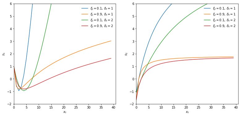
7Figure 1: News impact curves
The first element (left panel) and second element (right panel) of st in (7) is plotted against xt for different
values of ξt and δt .
Ft−1 ; ft , θ] = E[−∂∇t /∂ft0 | Ft−1 ; ft , θ], such that the conditional variance of st is equal to
the unit matrix. For the GPD, we have
−1
1 + ξt 0
Lt = √
, (6)
−1 1 + 2ξt
see Appendix A.2 for a derivation. Combining terms yields the scaled score as
δt − (ξt + 3 + ξt−1 ) · xt
ξ −2 (1 + ξt ) · log 1 + ξt δ −1 xt +
t t
δt + ξt xt
st = L0t ∇t =
. (7)
√ x t − δt
1 + 2ξt
δt + ξt xt
Though the scaled score in (7) seems unstable at first sight for ξt near zero, the expression
actually has a finite limit equal to limξt ↓0 s1,t = 1 − 2δt−1 xt + 12 δt−2 x2t .
Figure 1 plots the two elements of (7) as a function of xt for different values of ξt and δt .
The behavior of the scaled score is intuitive: Large xt imply that ft is adjusted upwards. For
high realization of xt the adjustments are greatest when the current tail shape and tail scale
are low. The function shapes become increasingly concave as x → ∞ in line with robust
updates of the time-varying parameters. This distinguishes our current set-up sharply from
8an approach directly based on quantile functions; see Patton et al. (2019) and Catania and
Luati (2019), in particular for risk measures such as ES. In Patton et al. (2019), ES reacts
linearly to the VaR exceedance.This can result in noisy or unstable ES estimates. Using the
GPD shape as emanating from EVT, Figure 1 shows that ξt and δt react more modestly to
large POT observations. This makes sense, as we expect such ‘outliers’ to occur more often
for higher values of ξt . For extremely high ξt ≥ 1, the ES even ceases to exist. We also note
that small realizations of xt imply downward adjustments of both elements of ft , up to the
point where xt becomes very small. In that case ftξ is adjusted upward, as observations near
the center of a fat-tailed distribution signal increased peakedness (=leptokurtosis); see also
Lucas and Zhang (2016). The score-driven steps in (7) can thus result in more stable and
interpretable parameter paths due to the concavity of the news impact curves.
When there is no tail observation, i.e. xt = εt − τ ≤ 0, then the new observation carries
no information about ξt and δt ; see McNeil et al. (2010, Chapter 7). In such cases we set the
score to zero, and continue to use (4) to update ft .3 Long consecutive stretches of zero scores
can lead to erratic paths for ft and thus (ξt , δt ). In addition, such stretches of zero scores can
be problematic for inference on θ; see Blasques et al. (2018). Both issues can be addressed by
taking into account lagged values of the scaled score via the exponentially-weighted moving
average specification
ft+1 = ω + As̃t + Bft , (8)
where s̃t = (1 − λ)st + λs̃t−1 , λ ∈ (0, 1) is an additional parameter to be estimated, and st
is given by (7). While st is most often zero, s̃t is not. Clearly, (4) is a special case of (8) for
λ → 0. Specification (8) leads to a GAS(1,2) specification for ft ,
I2 − B L (1 − λ)−1 1 − λL ft+1 = ω + Ast ,
where L is the lag operator. To see this, first rewrite (8) to (I2 − B L)ft+1 = ω + As̃t , and
then multiply both sides by (1 − λ L)/(1 − λ), using (1 − λ L)s̃t = (1 − λ)st . The smoothing
3
If ω = 0, B = I2 , and p = q = 1 in (4), then a zero score implies that both tail parameters retain their
current values. We adopt this specification in Section 4 below.
9approach in (8) is similar to the approach in Patton (2006) that uses up to ten lags of the
driver (in our case the score) to smooth the dynamics of the time-varying parameter.
The transition equation for ft can be extended further if additional conditioning variables
are available. For example, central bank sovereign bond purchases may help explain the time-
variation in the tail shape and tail scale parameters associated with changes in sovereign bond
yields; see Section 4. Such additional variables can be taken into account in a straightforward
way via the modified transition equation,
ft+1 = ω + As˜t + Bft + C · zt , (9)
where all explanatory variables are stacked into vector zt , and C is a conformable matrix of
impact coefficients that needs to be estimated.
We consider three different ways to set the relevant thresholds. The thresholds can
be either time-invariant (τ ) or time-varying (τt ). The construction of the thresholds can be
important in practice because τt determines whether an observation lies in the tail, and, if so,
what is the magnitude of the exceedance xt = εt − τt > 0. The κ-quantile Qκ1:T ({ε1 , . . . , εT })
associated with the full sample is an obvious first candidate, κ ∈ (0, 1). In this case, τ =
Qκ1:T ({ε1 , . . . , εT }) is time-invariant. Alternatively, we can compute the quantile recursively
up to time t and set τt = Qκ1:t ({ε1 , . . . , εt }), such that τt is time-varying. Finally, we consider
a dynamic specification as suggested by Patton et al. (2019), according to which
τt+1 = τt + aτ · (1{εt > τt } − (1 − κ)) , (10)
where aτ is a parameter to be estimated, and τ1 = Qκ1:T is used to initialize the process.
The recursive specification (10) is a martingale since E[1{εt > τt } | Ft−1 , θ] = (1 − κ). The
threshold τt can now respond to changes in the underlying location, scale, and higher-order
moments of εt in a straightforward way. This is particularly relevant if the data yt is not
pre-filtered based on an appropriate location–scale model in a first step, for instance if we
set µt = 0 and σt = 1 in (1), thus modeling the conditional extreme tail shape of yt directly.
10We close this section with a brief comment on parameter interpretability. The tail shape
parameter ξt can always be interpreted as observation yt ’s contemporaneous inverse tail
index αt−1 . By contrast, the estimated scale parameter δt need not have a straightforward
interpretation in terms of yt ’s conditional variance. For example, assume that yt were GPD
distributed with time-varying tail shape parameter αt−1 and scale σt . We can then show that
the derived POT xt also has an exact GPD-distribution, with the same tail shape parameter
ξt = αt−1 , but a different scale parameter δt,τ = σt + αt−1 · τ ; see Web Appendix B.1 for
details. As a result, δt,τ increases with the threshold, varies positively with the tail shape
parameter ξt , and, importantly, should not be expected to provide a consistent estimate of
σt . A similar result can be derived if the time series data yt were Student’s t-distributed with
scale σt and tail index αt ; see Web Appendix B.2. We return to this issue in our simulation
Section 3, where we consider pseudo-true values of both parameters to benchmark how well
the model can estimates these.
2.2 Confidence bands for tail shape and scale
Confidence (or standard error) bands allow us to visualize the impact of estimation uncer-
tainty associated with the maximum likelihood estimate θ̂ on the filtered estimates fˆt (θ̂),
and, by extension, also (ξˆt , δ̂t )0 = exp(fˆt (θ̂)). Quantifying the uncertainty about these param-
eter paths is important, as classical EVT estimators of time-invariant tail shape parameters
are already typically associated with sizeable standard errors; see e.g. Hill (1975) and Huis-
man et al. (2001). Our confidence bands are based on the variance of fˆt , which we denote
Vt = Var(fˆt ). There exist two possible ways to construct these bands. Delta-method-based
bands can be devised using a linear approximation of the non-linear transition function for
ft , thus extending Blasques et al. (2016, Section 3.2) to the case of multiple lags. We provide
the equations in Web Appendix C. In our empirical application below, however, the linear
approximations are typically insufficient to capture the uncertainty in the highly non-linear
dynamics for some countries. As a result, delta-method-based bands can become unstable.
Therefore, we instead use simulation-based bands as in Blasques et al. (2016, Section 3.3).
Simulation-based confidence bands build on the asymptotic normality of θ̂. In particular,
11we draw S parameter values θ̂s , s = 1, . . . , S from the distribution N(θ̂, Ŵ ), where Ŵ is the
estimated covariance matrix of θ̂, e.g., a sandwich covariance matrix estimator. If the finite-
sample distribution of θ̂ were known, that could be used instead. For each draw θ̂s we now
run the filter for ft from t = 1 to t = T , thus obtaining S paths fˆts , for s = 1, . . . , S and
t = 1, . . . , T . These paths account automatically for all non-linearities in the dynamics for ft .
The simulated bands can now be obtained directly by calculating the appropriate percentiles
for each t over the S draws of the paths fˆts for s = 1, . . . , S.
2.3 Parameter estimation
Parameter estimates can be obtained in a standard way by numerically maximizing the log-
likelihood function. Observation-driven time series models such as (3) – (10) are attractive
because the log-likelihood is known in closed form. For a given set of time series observations
x1 , . . . , xT , the vector of unknown parameters θ can be estimated by maximizing the log-
likelihood function with respect to θ. The average log-likelihood function is given by
T
X
∗ −1
L (θ|FT ) = (T ) 1{xt > 0} · ln p(xt ; δt , ξt )
t=1
T
∗ −1
X 1 xt
= (T ) 1{xt > 0} · − ln(δt ) − 1 + ln 1 + ξt , (11)
t=1
ξt δt
PT
where T ∗ = t=1 1{xt > 0} is the number of POT values in the sample. Maximization of
(11) can be carried out using a conveniently chosen quasi-Newton optimization method.
Blasques et al. (2020) provide conditions under which the maximum likelihood estimator
of θ is consistent and asymptotically normally distributed within the class of correctly-
specified score-driven models. They also prove that (quasi-)maximum likelihood estimation
of θ can remain consistent (to pseudo-true values) and asymptotically normal even if the
score-driven model is misspecified in terms of ln p(xt ; ft ). This is reassuring since the GPD is
never exact for any finite value of τ < ∞. In the presence of misspecification, score updates
continue to minimize the local Kullback-Leibler divergence between the true conditional
density and the model-implied conditional density, and remain optimal in this sense; see
12Blasques et al. (2015). The asymptotic covariance matrix W = Var(θ̂) then takes its usual
sandwich form; see e.g. Davidson and MacKinnon (2004, Ch. 10) and Blasques et al. (2020).
The autoregressive parameter aτ in (10) cannot be estimated using (11). Another objec-
tive function is needed in this case. We suggest using the average quantile regression check
function of Koenker (2005, Ch. 3). The optimization problem can be formulated as
T
X T
X
−1 −1
min
τ
T ρκ (t − τt ) ⇐⇒ min
τ
T (t − τt ) (κ − 1{t < τt })
{a } {a }
t=1 t=1
XT
⇐⇒ max
τ
T −1 (t − τt ) ((1 − κ) − 1{t > τt }) , (12)
{a }
t=1
where ρκ (ut ) = ut (κ − 1{ut < 0}), and τt evolves as in (10). See also Engle and Manganelli
(2004) and Catania and Luati (2019) for the use of this objective function in a different
dynamic context. In practice, we estimate all thresholds τt via (12) before maximizing (11).4
2.4 A conditional location–scale–df model
This section introduces a score-driven location–scale–df model that can be used to pre-filter
univariate time series data yt that is arbitrarily fat-tailed, where df denotes the degrees of
freedom. The model modifies the setting of Lucas and Zhang (2016) with a Student’s t
distribution with time-varying volatility and degrees of freedom parameters to a setting that
also allows for a time-varying location µt parameter and to more extreme tails (νt < 2), in
which case the volatility no longer exists, but a time varying scale parameter σt > 0 does
exist. Since all parameters are time-varying, using this model minimizes the risk of mistaking
time-variation in the center of the distribution for time-variation in the tail, and vice versa.
The restriction νt > 0 aligns closely with the assumption αt > 0 and ξt > 0 in Section 2.1.
4
Numerical gradient-based optimizers, such as e.g. MaxBFGS, may only indicate weak convergence at
the optimum of (12). This is due to the piecewise linear objective function. The optimizer at hand may
not be suited for such a function, and will end up in a kink. This is not a problem, assuming we are not
interested in standard errors for aτ . Alternatively the interior point algorithm of Koenker and Park (1996)
could be used.
13For the purposes of pre-filtering, in this section yt is assumed to be generated by
yt ∼ t(yt ; µt , σt , νt ), (13)
p
where µt = E[yt | Ft−1 ] if νt > 1, and νt /(νt − 2) σt is the conditional volatility of yt if
νt > 2. All time-varying parameters are modeled in a score-driven way as
µt+1 = ω µ + aµ sµt + bµ µt + cµ zt + dµ yt , (14)
ln σt+1 = ω σ + aσ sσt + bσ ln σt + cσ zt + dσ 1{yt > µt }sLev
t , (15)
νt+1 = ω ν + aν sνt + bν νt + cν zt , (16)
where ω (·) , a(·) , b(·) , c(·) , and d(·) are scalar parameters to be estimated, and zt is a vector of
additional conditioning variables which may be available. The required scaled scores are
(νt + 3)(yt − µt )
sµt = , (17)
νt + σt−2 (yt − µt )2
(νt + 1)(yt − µt )2
σ νt + 3
st = · −1 , (18)
2νt νt σt2 + (yt − µt )2
−1
ν 1 νt 00 νt + 1 νt 00 νt 1 νt + 5
st = γ − γ +
2 4 2 4 2 2 (νt + 1)(νt + 3)
(yt − µt )2 (yt − µt )2
1 0 νt
0 νt + 1 νt + 1
+γ −γ + ln 1 + − , (19)
νt 2 2 νt σt2 νt νt σt2 + (yt − µt )2
where the functions γ 0 (x) and γ 00 (x) are the first and second derivatives of the log-gamma
function. We refer to Web Appendix D for a derivation of (17) – (19).
The “leverage” term dσ · 1{yt > µt }sLev
t in (15) allows ln σt+1 to be higher (or lower,
depending on the sign of dσ ) when yt is above its location µt . The term sLev
t = sσt (yt )−sσt (µt )
is constructed such that the score is continuous at µt . Leverage specifications are often
found to be valuable in many empirical applications; see e.g. Engle and Patton (2001). The
deterministic parameters in (14) – (16) can be estimated by (quasi-)maximum likelihood
methods in line with the discussion in Section 2.3.
142.5 Market risk measures
Market risk measurement is a major application of EVT methods in practice; see Manganelli
and Engle (2004) and McNeil et al. (2010). We consider the conditional VaR and conditional
ES as measures of one-step-ahead market risk. The GPD approximation (2) – (3) yields
useful closed-form estimators of the VaR and ES for high upper quantiles γ > G(τ | Ft−1 );
see McNeil and Frey (2000) and Rocco (2014). We can estimate the 1 − γ tail probability of
yt based on the GPD cdf for xt , obtaining
" −ξt #
1−γ
VaR (t | Ft−1 , θ) = τt + δt ξt−1
γ
−1 ,
t∗ /t
VaRγ (yt | Ft−1 , θ) = µt + σt VaRγ (t | Ft−1 , θ), (20)
where µt and σt are defined below (1), and t∗ is the number of observations of xt > 0 up to
time t, i.e., the number of observations ys for s = 1, . . . , t for which ys > τs . Put differently,
t∗ /t is an estimator of the tail probability κt = G(τt | Ft−1 ).
The conditional ES is the average conditional VaR in the tail across all quantiles γ (see
McNeil et al., 2010, Chapter 2), provided ξt < 1. The closed-form expressions are
Z 1
γ 1
ES (t | Ft−1 , θ) = VaRγ̃ (t | Ft−1 , θ)dγ̃
1−γ γ
VaRγ (t | Ft−1 , θ) δt − ξt τt
= + ,
1 − ξt 1 − ξt
ESγ (yt | Ft−1 , θ) = µt + σt ESγ (t | Ft−1 , θ); (21)
see Web Appendix E for a derivation of (20) – (21). The ESγ (yt | · ) is strictly higher than the
VaRγ (yt | · ) at the same confidence level, as it “looks further into the tail.” It can be shown
that the ratio ESγ (yt | · )/VaRγ (yt | · ) increases monotonically in ξt for γ → 1, indicating
that expected losses beyond the VaR become increasingly worse for heavier-tailed (higher
ξt ) distributions. Maximum likelihood estimators of the conditional VaR and conditional ES
can be obtained by inserting filtered estimates of µt , σt , ξt and δt into (20) and (21).
15For later reference, the sensitivity of VaRγ (yt ) to bond purchases zt−1 is given by
dVaRγ (yt ) ∂VaR dµt ∂VaR dσt d ln σt ∂VaR dδt dftδ ∂VaR dξt dftξ
= + + + .
dzt−1 ∂µt dzt−1 ∂σt d ln σt dzt−1 ∂δt dftδ dzt−1 ∂ξt dftξ dzt−1
The expression is intuitive: extreme upper quantiles can change if bond purchases zt−1 affect
the conditional location µt , the conditional scale σt , the tail scale δt , or the tail shape ξt .
The derivative is given by
dVaRγ (yt )
=cµ + σt VaRγ (t )cσ + σt (VaRγ (t ) − τt ) cδ
dzt−1
( −ξt )
1 − γ 1 − γ
−σt VaRγ (t ) − τt + δt ln cξ , (22)
t∗ /t t∗ /t
where µt and σt are given by (14) and (15), ftξ and ftδ are given by (9) with C = (cδ , cξ )0 .
3 Simulation study
This section studies the question whether our score-driven modeling approach can reliably
recover the time series variation in tail shape and tail scale in a variety of potentially chal-
lenging settings. In addition, we are interested in how to best choose the thresholds τt , as
well as the accuracy of EVT-based market risk measures when used in combination with our
modeling approach.
3.1 Simulation design
Our simulation design considers D = 2 different densities (GPD and t), P = 4 different
parameter paths for tail shape and tail scale, and H = 3 different ways to obtain the
appropriate thresholds τt . This yields 2 × 4 × 3 = 24 simulation experiments. In each
experiment, we draw S = 100 univariate simulation samples of length T = 25, 000. We focus
on the upper 1 − κ = 5% tail. As a result, approximately 25, 000 · 0.05 = 1, 250 observations
are available in each simulation to compute informative POTs xt > 0. The time series
dimension T is chosen to resemble that of the empirical data considered in Section 4.
16GPD and t-densities: We first simulate yt from a GPD distribution with time-varying tail
shape αt−1 and tail scale σt , yt ∼ GPD(αt−1 , σt ). We then consider a Student’s t distribution
with time-varying scale σt and degrees of freedom αt , yt ∼t(0, σt , αt ). POT values xt are
obtained as xt = yt − τt .
Parameter paths: We consider four different paths for the tail shape αt−1 and tail scale σt
parameters. For both GPD and t densities we consider
(1) Constant: αt−1 = 0.5, σt = 1;
(2) Sine and constant: αt−1 = 0.5 + 0.3 sin(4πt/T ), σt = 1;
(3) Slow sine and frequent sine: αt−1 = 0.5 + 0.3 sin(4πt/T ), σt = 1 + 0.5 sin(16πt/T );
(4) Synchronized sines: αt−1 = 0.5 + 0.3 sin(4πt/T ), σt = 1 + 0.5 sin(4πt/T ).
Path (1) considers the special case of time-invariant tail shape and scale parameters. Natu-
rally, we would want our dynamic framework to cover constant parameters as a special case.
Path (2) allows the tail shape to vary considerably between 0.2 and 0.8, while keeping the
scale (volatility) of the data constant. This parameter path corresponds to the empirical
practice of working with volatility pre-filtered data. Path (3) stipulates that both parame-
ters vary over time. Finally, Path (4) considers the case of synchronized variation in both
parameters. This setting may be particularly challenging for two reasons. First, the tail
observations occur most frequently when both tail shape and scale are high, making it po-
tentially difficult to disentangle the two effects. Second, less information about the tail is
available when both parameters are low simultaneously.
Different thresholds: We consider three thresholds τt . First, we use the true time-varying
95%–quantile based on our knowledge of the true density and of αt and σt . This constitutes
an infeasible best benchmark. Second, we construct τt as the 95%–quantile of the expanding
window of data up to time t, i.e. τt = Q0.95
1:t ({ε1 , . . . , εt }). Finally, we use the recursive
specification (10), with aτ fixed at 0.25, and initialized at τ1 = Q1:T
0.95
.
Evaluation metrics: Our main metric for evaluating model performance is the root
PS q 1 PT ˆ
mean squared error RMSE = S s=1 T t=1 (ξst − ξ¯st )2 , where ξˆst is the estimated tail
1
17shape parameter in simulation s, ξ¯st is the corresponding (pseudo-)true tail shape, s =
1, . . . , S denotes the simulation run, and t = 1, . . . , T is the number of observations in
each draw. The RMSE for the tail scale parameter δt is obtained analogously, RMSE =
1
PS q 1 PT 2
S s=1 T t=1 (δ̂st − δ̄st ) , where δ̄st denotes the pseudo-true value of δst . The pseudo-true
values ξ¯st and δ̄st are obtained by numerically minimizing the Kullback-Leibler divergence
between the GPD and the data generating process beyond the true time-varying 95% quan-
tile τt . As the true conditional density is known at all times in a simulation setting, these
pseudo-true benchmarks are easily computed. We note that particularly the GPD scale pa-
rameter δ̄t may have very different dynamics from σt , as it combines dynamics in αt and σt
via the EVT limiting expression in (2).
3.2 Simulation results
Table 1 presents root mean squared error (RMSE) statistics for tail shape ξˆs,t , tail scale δ̂s,t ,
and Value-at-Risk VaR
d s,t estimates. Figures F.1 and F.2 in Web Appendix F.1 compare
d 0.99 , and ES
median estimated parameter paths for ξˆt , ξˆt , VaR c 0.99 to their (pseudo-)true
values. Figure 2 is a representative example of the simulation outcomes when yt is generated
by a Student’s t distribution.
We focus on three main findings. First, all models seem to work well in recovering the
true underlying ξt and δt dynamics. The median estimates in Figures F.1 and F.2 tend to
be close to their (pseudo-)true values. Particularly the sometimes highly non-linear patters
of δt are recovered well. The model also captures well the peaks of ξt , so the fattest tails.
The model needs some time to recognize that the extreme tail has become more benign, i.e.,
that ξt has gone down. The good fit is corroborated by Table 1. Both estimation methods
for τt only loose about 10% RMSE for ξt and δt compared to the use of the true (infeasible)
τt .
Second, when comparing the recursive estimate τ̂t versus the dynamic τt∗ of Patton et al.
(2019) in Table 1, differences are mostly small and insignificant. If there is no time-variation
(path (1)), the recursive estimate does slightly better, as expected. The converse is true for
δt if the true parameters vary over time.
18Table 1: Simulation RMSE results
Root mean squared error (RMSE) statistics for two different distributions (GPD and t, in columns) and
for four different parameter paths for tail shape ξt and tail scale δt (paths (1) – (4), in rows). Thresholds
τt , τ̂t , and τ̂t∗ denote i) the infeasible true time-varying threshold, ii) the empirical quantile associated
with an expanding window of observations y1 , . . . , yt , and iii) the estimated conditional quantile using
(12) with aτ = 0.25, respectively. We consider 100 simulations for each DGP, and a time series of 25, 000
observations in each simulation. Model performance is measured by the RMSE from the true ξ¯t and δ̄t in
each draw. For VaR, model performance is measured in relative terms as RMSE rescaled by the squared VaRt .
Model GPD(τt ) GPD(τ̂t ) GPD(τ̂t∗ ) t(τt ) t(τ̂t ) t(τ̂t∗ )
(infeasible) (infeasible)
RMSE ξˆs,t
(1) 0.000 0.000 0.000 0.000 0.000 0.000
(0.000) (0.000) (0.000) (0.000) (0.000) (0.000)
(2) 0.171 0.177 0.178 0.182 0.188 0.189
(0.002) (0.002) (0.002) (0.002) (0.002) (0.002)
(3) 0.182 0.188 0.189 0.190 0.197 0.197
(0.002) (0.002) (0.002) (0.002) (0.002) (0.002)
(4) 0.177 0.186 0.183 0.188 0.195 0.192
(0.002) (0.002) (0.002) (0.002) (0.002) (0.002)
RMSE δ̂s,t
(1) 0.005 0.014 0.068 0.005 0.010 0.034
(0.003) (0.006) (0.013) (0.002) (0.004) (0.006)
(2) 1.646 1.774 1.753 0.580 0.589 0.588
(0.034) (0.040) (0.036) (0.013) (0.012) (0.013)
(3) 2.421 2.913 2.813 0.836 0.960 0.924
(0.054) (0.054) (0.049) (0.015) (0.020) (0.017)
(4) 2.608 2.904 2.844 0.925 0.970 0.964
(0.057) (0.059) (0.059) (0.020) (0.020) (0.022)
RMSE VaR
d s,t
(1) 0.001 0.003 0.016 0.124 0.124 0.149
(0.001) (0.002) (0.003) (0.001) (0.001) (0.002)
(2) 0.924 0.987 0.964 0.249 0.243 0.257
(0.027) (0.032) (0.031) (0.003) (0.003) (0.003)
(3) 1.063 1.304 1.209 0.322 0.344 0.349
(0.025) (0.041) (0.033) (0.004) (0.005) (0.004)
(4) 1.020 1.120 1.083 0.302 0.297 0.319
(0.027) (0.028) (0.028) (0.003) (0.003) (0.003)
Third, Figure 2 as well as Figures F.1 and F.2 in Web Appendix F.1 corroborate that our
EVT-based market risk measures, such as VaR and ES at a high confidence level γ = 0.99,
tend to be estimated sufficiently accurately when used in combination with our modeling
approach. The low and high frequency dynamics of the VaR and ES are both captured
well. There only appears some under-estimation of the ES at its very peak where tails
are extremely fat. Overall, we conclude that the model captures well the dynamics of the
19Figure 2: Simulation results: a representative example
Time series data is here generated as yt ∼t(0, σt , αt ), where αt−1 = 0.5 + 0.3 sin(4πt/T ) and σt = 1 +
0.5 sin(16πt/T ). This is Path 3 in Section 3.1. Pseudo-true parameter values are reported in solid red. The
four panels report estimates of ξt , δt , VaRt , and ESt , respectively. Median filtered values are plotted in solid
black. The first two panels also indicate the lower 5% and upper 95% quantiles of the estimates (black dots).
The time-varying threshold τ̂t is estimated based on the recursive specification (10) in conjunction with the
objective function (12).
Tail shape estimates ξ^ t Tail scale estimates δ^ t VaR 99% ES 99%
ξ t median δ t median VaR 99% median ES 99% median
true value 10 true value true value true value
100
1.0 20
Path 3
5
10 50
0.5
0 12500 25000 0 12500 25000 0 12500 25000 0 12500 25000
tails, even if the model does not coincide with the data generating process and is therefore
misspecified.
4 The tail impact of Eurosystem asset purchases
4.1 Data
4.1.1 High-frequency data on bond yields
We obtain high-frequency data on changes in euro area sovereign bond yields from Thomson
Reuters/Datastream, focusing on Spanish (EN), Greek (GR), Irish (IE), Italian (IT), and
Portuguese (PT) five-year sovereign benchmark bonds. These market segments were among
the most affected by the euro area debt crisis; see e.g. ECB (2014). SMP bond purchases
undertaken during the debt crisis predominantly targeted the two- to ten-year maturity
bracket, with the five-year maturity approximately in the middle of that spectrum. We
focus on the impact on five-year benchmark bonds for this reason. We model the midpoint
between ask and bid prices. Bond prices are expressed in yields-to-maturity and are obtained
from continuous dealer quotes.
20Our sample ranges from 04 January 2010 to 31 December 2012, covering the most in-
tense phase of the euro area sovereign debt crisis. The bond yields are sampled at the
15-minute frequency between 8AM and 6PM. Following Ghysels et al. (2017) we do not
consider overnight changes in yield, such that the first 15-minute interval covers 8AM to
8:15AM. This yields 40 intra-daily observations per trading day. This yields 40 intra-daily
observations per day, with T ≈ 3 × 260 × 40 ≈ 31, 000 observations per country.
The Greek data are an exception. Greek bonds experienced a credit event on 09 March
2012. In January and February 2012 the five-year benchmark bond continued trading, infre-
quently and at low prices, until approximately one week before the credit event. Our Greek
data sample ends on 02 March 2012 for this reason. We include the Greek pre-default data
as a truly extreme case, allowing us to “stress-test” our EVT estimation methodology.
Figure F.3 in the Web Appendix F.2 plots the yield-to-maturity of our five benchmark
bond yields in levels and in first differences. All five yields exhibited large and sudden moves,
leading to volatility clustering and extreme realizations of yield changes during the euro area
sovereign debt crisis.
Table 2 provides summary statistics for changes in our five benchmark bond yields sam-
pled at the 15-minute frequency. All time series have significant non-Gaussian features under
standard tests and significance levels. In particular, we note the non-zero skewness and large
values of kurtosis for almost all time series in the sample. Yield changes are covariance sta-
tionary according to standard unit root (ADF) tests. Most yield changes are below one bps
in absolute value. This suggests that the data are not only heavy-tailed, but also extremely
peaked around zero in the center. The pronounced non-Gaussian data features strongly
suggest a non-Gaussian empirical framework for modeling conditional location, dispersion,
and higher-order moments.
4.1.2 High–frequency data on Eurosystem bond purchases
We study the impact of SMP bond purchases between 2010 and 2012 for five euro area coun-
tries: Greece, Ireland, Italy, Portugal, and Spain. At the end of our sample, the Eurosystem
held e99.0 bn in Italian sovereign bonds, e30.8 bn in Greek debt, e43.7 bn in Spanish debt,
21Table 2: Data descriptive statistics
Summary statistics for changes in five-year sovereign benchmark bond yields measured in percentage points.
Columns labeled EN, GR, IE, IT, and PT refer to Spanish, Greek, Irish, Italian, and Portuguese five-year
benchmark bond yields. The sample ranges from 04 January 2010 to 28 December 2012. The Greek
sample ends on 02 March 2012. Reported p-values for skewness and kurtosis refer to D’Agostino et al.
(1990)’s test. The last row reports the fraction of yield changes smaller than one basis point in absolute value.
EN GR IE IT PT
Median 0.00 0.00 0.00 0.00 0.00
Std. dev. 0.02 0.46 0.06 0.03 0.08
Minimum -0.74 -20.73 -0.91 -0.39 -1.15
Maximum 0.47 14.77 1.45 0.43 1.20
Skewness -42.29 -104.76 34.11 14.91 12.40
Skew. p-value 0.00 0.00 0.00 0.00 0.00
Kurtosis 357.94 195.05 301.26 293.40 279.44
Kurt. p-value 0.00 0.00 0.00 0.00 0.00
Fraction yt < 1 bp 81% 77% 81% 81% 77%
e21.6 bn in Portuguese debt, and e13.6 bn in Irish bonds; see the ECB (2013)’s Annual
Report. The SMP’s daily cross-country breakdown of the purchase data is still confidential
at the time of writing. We use the country-specific data on SMP purchases when studying
the impact of the program.
The SMP had the objective of helping to restore the monetary policy transmission mech-
anism by addressing the malfunctioning of certain government bond markets. The SMP
consisted of interventions in the form of outright secondary market purchases. Implicit in
the concept of malfunctioning markets is the notion that government bond yields can be
unjustifiably high and volatile.
Figure 3 plots weekly total SMP purchases across countries as well as their accumulated
book value over time. Approximately e214 billion (bn) of bonds were acquired within
the SMP between 2010 and early 2012. The SMP was announced on 10 May 2010 and
initially focused on Greek, Irish, and Portuguese debt securities. The program was extended
to include Italian and Spanish bonds on 8 August 2011. The SMP was replaced by the
Outright Monetary Transactions (OMTs) program on 6 September 2012; see Cœuré (2013).
Visibly, the purchase data are unevenly spread over time. Between 10 May 2010 and Spring
2012 there are long periods during which the SMP was open but inactive.
22Figure 3: Weekly and total SMP purchase amounts.
The figure plots the book value of settled SMP purchases as of the end of a given week. We report weekly
purchases across countries (left panel) as well as the cumulative amounts (right panel). Maturing amounts
are excluded.
C:\RESEARCH\GAStails\Bond_Stata\OXrw_Final\Draft_2017Feb22\purchases1bn_2015.eps 02/22/17 19:38:38
250
Weekly purchases, book value
Total purchases, book value
20 200
200
150
150
bn EUR
bn EUR
10 100
100
50
50
2010 2011 2012 2010 2011 2012
The SMP purchase data are time-stamped, allowing us to construct time series data
zt of country-specific SMP purchases at the high (15-minute) frequency. The 15-minute
frequency is chosen because 15 minutes is the regulatory limit for the recording of trades
by the Eurosystem. Observations zt contain all sovereign bond purchases at par (nominal)
value between t − 1 and t for the respective country, not only purchases of the five-year
benchmark bond.
4.2 Location–scale–df model estimates
This section applies our novel location–scale–df model of Section 2.4 to study changes in the
yield-to-maturity of five-year sovereign benchmark bonds as discussed in Section 4.1.1. We
are particularly interested in each series’ location, scale, and degrees of freedom, and how
these respond to Eurosystem bond purchases.
We apply the model to the raw data series after removing a (negligible) intra-daily pattern
via dummy variable regression. We introduce two simplifications to the general specification.
First, preliminary analyses suggest that the location parameters are approximately time-
invariant, such that aµ and bµ are close to zero. We proceed by imposing this restriction.
Note that the specification for the mean still includes dµ · yt−1 to accommodate a potentially
23Table 3: Parameter estimates for the location–scale–df model
Parameter estimates for the univariate location–scale–df model (13). Rows labeled EN, GR, IE, IT, and
PT refer to Spanish, Greek, Irish, Italian, and Portuguese five-year benchmark bond yields. The estimation
sample ranges from 04 January 2010 to 28 December 2012 for all countries except Greece. Standard error
estimates are in round brackets and are taken from a sandwich covariance matrix. P-values are provided in
square brackets.
EN GR IE IT PT
ωµ 0.013 -0.038 0.003 -0.003 -0.016
(0.007) (0.024) (0.005) (0.007) (0.006)
[0.046] [0.108] [0.641] [0.618] [0.004]
cµ -2.623 -2.856 0.017 -1.479 -0.053
(SMP) (0.941) (2.483) (1.594) (0.552) (2.068)
[0.005] [0.250] [0.992] [0.007] [0.980]
dµ -0.039 -0.000 -0.010 -0.029 -0.004
(AR1) (0.007) (0.000) (0.002) (0.010) (0.001)
[0.000] [0.200] [0.000] [0.004] [0.003]
aσ 0.107 0.141 0.135 0.124 0.089
(0.015) (0.011) (0.012) (0.013) (0.011)
[0.000] [0.000] [0.000] [0.000] [0.000]
cσ -0.126 -0.055 -0.461 -0.049 -0.441
(SMP) (0.089) (0.115) (0.324) (0.050) (0.228)
[0.158] [0.635] [0.155] [0.325] [0.053]
dσ 0.004 -0.004 -0.000 0.005 -0.000
(LEV) (0.001) (0.001) (0.001) (0.002) (0.001)
[0.006] [0.001] [0.885] [0.002] [0.641]
aν 0.004 0.018 0.007 0.006 0.008
(0.001) (0.002) (0.001) (0.001) (0.001)
[0.000] [0.000] [0.000] [0.000] [0.000]
cν 0.031 0.042 0.022 0.013 0.000
(SMP) (0.014) (0.027) (0.035) (0.007) (0.028)
[0.033] [0.122] [0.530] [0.052] [0.993]
loglik -56226.2 -68788.4 -68584.7 -56218.6 -78164.0
AIC 112468.4 137592.9 137185.4 112453.2 156343.9
BIC 112534.9 137656.8 137252.0 112519.8 156410.6
negative serial correlation at the 15-minute frequency; see e.g. Roll (1984). Second, we find
that the persistence (bσ and bν ) in volatility and degrees of freedom parameters is very high.
We therefore set ω σ = ω ν = 0 and bσ = bν = 1, thus adopting the EWMA restricted score
dynamics of Lucas and Zhang (2016) for the scale and df parameters. A comparison of model
selection criteria (AIC, BIC) across model specifications confirms these choices. With these
simplifications in place, Table 3 now presents the parameter estimates.
We focus on three findings in Table 3. First, SMP bond purchases tended to lower the
conditional location of future bond yields for most countries. The estimate of cµ is negative
24You can also read