Service Delivery, Corruption, and Information Flows in Bureaucracies: Evidence from the Bangladesh Civil Service - UCSB Department of ...
←
→
Page content transcription
If your browser does not render page correctly, please read the page content below
Service Delivery, Corruption, and Information Flows in

      Bureaucracies: Evidence from the Bangladesh Civil Service

                                                   Martin Mattsson∗

                                                   Job Market Paper
                                                 17th November 2020
                                            Click here for latest version

                                                          Abstract

      Government bureaucracies in low- and middle-income countries often suffer from corruption and
      slow public service delivery. Can an information system – providing information about delays to the
      responsible bureaucrats and their supervisors – reduce delays? Paying bribes for faster service deli-
      very is a common form of corruption, but does improving average processing times reduce bribes?
      To answer these questions, I conduct a large-scale field experiment over 16 months with the Bangla-
      desh Civil Service. I send monthly scorecards measuring delays in service delivery to government
      officials and their supervisors. The scorecards increase services delivered on time by 11% but do not
      reduce bribes. Instead, the scorecards increase bribes for high-performing bureaucrats. These results
      are inconsistent with existing theories suggesting that speeding up service delivery reduces bribes.
      I propose a model where bureaucrats’ shame or reputational concerns constrain corruption. When
      bureaucrats’ reputation improves through positive performance feedback, this constraint is relaxed,
      and bribes increase. Overall, my study shows that improving information within bureaucracies can
      change bureaucrats’ behavior, even without explicit incentives. However, positive performance feed-
      back can have negative spillovers on bureaucrats’ performance across different behaviors.

  ∗ Yale University, martin.mattsson@yale.edu. I would like to thank Gaurav Chiplunkar, Anir Chowdhury, Andrew Foster,
Eduardo Fraga, Sahana Ghosh, Marina Halac, Ashraful Haque, Enamul Haque, Daniel Keniston, Ro’ee Levy, Imran Matin,
Mushfiq Mobarak, Farria Naeem, Rohini Pande, Nick Ryan, Mark Rosenzweig, Jeff Weaver, Jaya Wen, Fabrizio Zilibotti, and
numerous seminar participants for helpful comments and suggestions. I also thank Mahzabin Khan and Ashraf Mian for
excellent research assistance, as well as IPA Bangladesh for outstanding research support. A randomized controlled trial regi-
stry and pre-analysis plan are available at: www.socialscienceregistry.org/trials/3232. This work was supported by the JPAL
Governance Initiative (GR-0861), the International Growth Centre (31422), the Yale Economic Growth Center, the MacMillan
Center for International and Area Studies, the Weiss Family Fund, and the Sylff fellowship.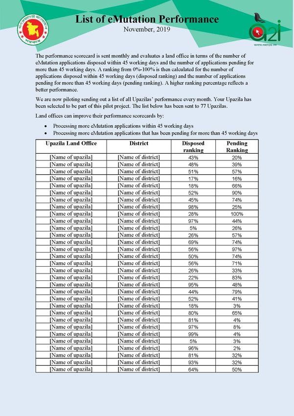
1   Introduction

The state’s capacity to implement its policies, secure property rights, and provide basic public services is

paramount for economic development. To have this capacity, the state needs a functioning bureaucracy

of government officials motivated to carry out their tasks. For career civil servants, compressed wage

structures, secure employment, and opportunities for rent extraction through corruption often lead to

weak or counterproductive incentives, especially in low- and middle-income countries. While explicit

incentive structures, such as pay-for-performance contracts, can change the behavior of government

officials, they are often hard to implement without unintended consequences (Finan, Olken, and Pande,

2017). Furthermore, political constraints often prevent the introduction of explicit incentive structures

altogether. However, the lack of explicit incentives does not mean that civil servants have no incentives.

Supervisors in government bureaucracies often influence future postings and career paths of lower-level

bureaucrats, which can be a strong motivating factor for civil servants (Khan, Khwaja, and Olken, 2019).

Furthermore, bureaucrats may have strong intrinsic motivations to perform their jobs well (Banuri and

Keefer, 2013; Cowley and Smith, 2014).

    Providing better information flows within bureaucracies about individual officials’ performance may

improve existing incentives by allowing supervisors to align postings and promotions more closely with

job performance. Regular feedback may also increase officials’ intrinsic motivation by making their own

performance more salient to themselves. Furthermore, the flexible interpretation of information that

is not directly tied to explicit incentives may avoid some of the common pitfalls of explicit incentives

structures such as the neglect of tasks not measured by the performance indicators and opposition from

individuals within the organization leading to poor implementation (Banerjee, Chattopadhyay, Duflo,

Keniston, and Singh, 2020). Historically, high-frequency information on bureaucrat performance has of-

ten been expensive to collect, but e-governance systems can substantially reduce this cost and increase

the data quality (Singh, 2020). As low- and middle-income countries have expanded their digital ca-

pabilities, this has created new opportunities for improved information systems in the management of

government officials.

    This paper focuses on the processing time of applications for changes to government land records in

Bangladesh. An update to the government records has to be made every time a parcel of land changes

owners and is necessary for the issuance of a land title to the new owner. Updated land records and land

titles are essential for individuals to have secure property rights over land. Land disputes are one of

                                                     2
the most severe legal problem in Bangladesh, with 29% of adults having faced a land dispute in the past
four years (Hague Institute for Innovation of Law, 2018). Slow public service delivery is also a significant
problem in Bangladesh. For example, only 56% of land record change applications in my control group
are processed within a 45 working day time limit mandated by the government. Furthermore, faster
service provision is a commonly stated reason for bribe payments, suggesting that slow service delivery
on average may cause corruption as some firms and citizens pay bribes to avoid having to wait for their
services.1
In an experiment with the Bangladesh Civil Service, I provide information regarding junior civil ser-
vants’ performance using monthly scorecards sent to the civil servants themselves and their supervisors.
The scorecards are designed to reduce delays in the processing of applications for land record changes
and are based on data from an e-governance system. There are two performance indicators shown on
the scorecards: the number of applications processed within the official time limit of 45 working days
and the number of applications pending beyond that limit. The scorecards also show the bureaucrats’
relative performance on these indicators, compared to all other bureaucrats in the experiment. The in-
tervention is randomized at the level of the land office, and there is only one civil servant per office.
The experiment was carried out at a large scale and involve 311 land offices (59% of all land offices in
Bangladesh), which serve a population of approximately 95 million people.
The scorecards had a meaningful effect on bureaucrats’ behavior. Using administrative data on more
than a million applications, I estimate that the scorecards increase the share of applications processed
within the time limit by 6 percentage points or 11%. The effect starts almost immediately after the
scorecards are first sent out and is present for the 16 month period of the experiment. The scorecards also
decreased the average processing time of applications by 13% and the applicants’ visits to government
offices by 12%. The effects are almost entirely driven by bureaucrats in offices with a below-median
performance at baseline, improving their performance. This result shows that improving the information
flows within a bureaucracy can change bureaucrats’ behavior, even without explicit incentive structures.
Since the scorecards were sent to both the bureaucrats and their supervisors, there might be two
different mechanisms for the effect on behavior. First, the bureaucrats may care about their reputation
among their supervisors, potentially because of the influence the supervisors have over their careers.
Second, the scorecards may also change bureaucrats’ behavior by causing a sense of shame or pride
through making their absolute and relative performance more salient to the bureaucrats themselves. For
1 Among households in Bangladesh reporting having paid a bribe for a public service, 23% stated that "timely service" was
one of the reasons for paying the bribe (Transparency International Bangladesh, 2018).
3ease of exposition, I will refer to these two concerns as reputational concerns. While I cannot distinguish
between these two mechanisms, I use a variation of the scorecard to test if peer effects from having
the performance information shared among bureaucrats at the same level within the bureaucracy can
motivate bureaucrats further than having the information shared only with the supervisors. I find no
evidence of meaningful peer effects beyond the effect of the standard scorecards.
Some existing theories of corruption suggest that the average speed of public service delivery is cau-
sally and negatively related to bribes since, when average processing times are long, some applicants pay
to avoid having to wait (Leff, 1964; Rose-Ackerman, 1978; Kaufmann and Wei, 1999). I conduct a survey
among applicants and use the experimental variation in processing times to test theories of how they
are related to corruption. Overall, the scorecards did not decrease bribe payments. The point estimate
of the effect is an increase of BDT 1,046 (~USD 12) or 17%, and the lower bound of the 95% confidence
interval is a decrease of 3%.2 The increase comes from a positive effect on the bribe amounts reported
(intensive margin) with no effect on the fraction of applicants reporting bribes (extensive margin). Using
an experimental information intervention among surveyed applicants, I rule out that the lack of a decre-
ase in bribes is due to the information about the improved processing times not yet having disseminated
among applicants.
The positive effect of the scorecards on bribe payments is concentrated among the offices that were
over-performing at baseline, i.e., the offices for which the scorecards have no effect on processing times.
In the under-performing offices, where scorecards improve processing times, they do not affect bribes.
This is inconsistent with a causal relationship between average processing times and bribes since pro-
cessing times can improve without bribes changing, and bribes can increase without processing times
changing.
I propose a model in which bureaucrats trade-off reputational concerns, bribe money, and the uti-
lity cost of effort. The bureaucrats’ reputation is determined by their visible job performance along two
dimensions, delays and bribe extraction, which are only imperfectly observable to supervisors. The
scorecards increase the visibility of delays and thereby make them more important for reputation. For
under-performing bureaucrats, this also means that the scorecards decrease their reputation. Therefore,
the model predicts that under-performing bureaucrats reduce delays by providing more effort. The mo-
del also predicts that when the scorecards highlight the already good performance of over-performing
bureaucrats, this relaxes their reputation constraint, allowing them to increase bribes. Furthermore, the
2 Throughout the paper, I use a USD/BDT exchange rate of 84.3, the average exchange rate during the experiment.
4model is consistent with the result that the scorecards do not affect delays for over-performing bureau-
crats. For them, more visible delays increase incentives to avoid delays (substitution effect), but incre-
ased reputation has made the marginal importance of reputation smaller (income effect), so the overall
effect is ambiguous.
This paper contributes to four strands of literature. First, it contributes to the literature on how
incentives shape bureaucratic performance. There is an extensive literature on both monetary and non-
monetary explicit incentives (e.g., Ashraf, Bandiera, and Jack, 2014; Khan, Khwaja, and Olken, 2016;
Khan et al., 2019). This paper contributes to the growing literature on the effects of information flows
within government bureaucracies (Dodge, Neggers, Pande, and Moore, 2018; Muralidharan, Niehaus,
Sukhtankar, and Weaver, 2020; Dal Bó, Finan, Li, and Schechter, 2019; Callen, Gulzar, Hasanain, Khan,
and Rezaee, 2020; Banerjee et al., 2020). In particular, I show that information flows about individual
civil servants’ performance can improve public service delivery even without explicit incentives and
that this effect is persistent over time. This could be due to long-term career concerns of bureaucrats
(Niehaus and Sukhtankar, 2013a; Bertrand, Burgess, Chawla, and Xu, 2020) or a sense of shame or pride
internal to the bureaucrats themselves (Allcott, 2011; Dustan, Maldonado, and Hernandez-Agramonte,
2018). However, I find no evidence that reputational concerns among bureaucrats at the same level in
the organizational hierarchy are a substantial motivating factor (Mas and Moretti, 2009; Cornelissen,
Dustmann, and Schönberg, 2017). My model suggests that reputational concerns provide incentives for
performance and limit the amounts of bribes collected by bureaucrats. However, the model also shows
how improving the relative reputation of individual bureaucrats can lead them to perform worse and be
more corrupt.
Second, the paper provides empirical evidence on the connection between corruption and the speed
of public service delivery, or more generally, red tape. Slow service delivery is positively associated with
corruption (Kaufmann and Wei, 1999; Freund, Hallward-Driemeier, and Rijkers, 2016), and applicants
may have to pay bribes to increase processing speed for services (Bertrand, Djankov, Hanna, and Mul-
lainathan, 2007). In the mainly theoretical literature on why the speed of service delivery and corruption
are associated, different models lead to drastically different policy conclusions. One view is that corrup-
tion allows firms and individuals to circumvent excessively onerous bureaucratic hurdles (Leff, 1964;
Huntington, 1968). In this view, rooting out corruption would decrease the speed of service delivery
and increase inefficiencies of excessive bureaucratic control. An opposing view is that corruption is the
driver of red tape and delays in public services, as making the de-jure regulation more onerous allows
5government officials to extract more bribes (Myrdal, 1968; Rose-Ackerman, 1978; Kaufmann and Wei,
1999).3 According to this view, we could improve service delivery by eliminating corruption. According
to both views, we could reduce corruption by providing services with fewer delays to everyone. I con-
tribute to the literature by showing that, in this context, increasing the average speed of service delivery
does not decrease bribe payments and that there is no evidence of a causal relationship between the
average speed of service delivery and bribes.
Third, the paper contributes to the literature on the determinants of bribe amounts. In some set-
tings, bribe payers’ outside option and ability to pay constrain bribe amounts (Svensson, 2003; Bai, Ja-
yachandran, Malesky, and Olken, 2019), potentially leaving little room for applicant complaints or mo-
nitoring to reduce corruption (Niehaus and Sukhtankar, 2013b). In other settings, monitoring has been
effective in reducing corruption (Reinikka and Svensson, 2005; Olken, 2007). I show that, in this context,
individual bureaucrats can increase bribes and that bribes do not just reflect the difference between the
official fee and the applicants’ willingness or ability to pay for the service. Instead, my model highlights
how bureaucrats’ reputational concerns constrain bribes, explaining why bribes are substantially below
applicants’ willingness to pay for the service.
Finally, the paper is related to the literature on the effects of e-governance in settings with low go-
vernment capacity. In some cases, e-governance systems have improved government efficiency and
reduced corruption (Banerjee, Duflo, Imbert, Mathew, and Pande, 2020; Lewis-Faupel, Neggers, Olken,
and Pande, 2016). While in others, they have not had substantial benefits and wasted scarce government
resources (World Development Report, 2016). This paper does not evaluate an e-governance system as
a whole. Instead, it provides evidence on the untapped potential in the data that e-governance systems
generate for the management of government officials.
The rest of the paper is organized as follows. Section 2 describes the context, experimental interven-
tions, and data. Section 3 describes the empirical strategy used to analyze the experiment. Section 4
presents the estimated effects of the scorecards on processing times and bribes. Section 5 discusses how
the results relates to existing theories of the relationship between the speed of service delivery and cor-
ruption. Section 6 proposes a model of bureaucratic behavior explaining the results. Section 7 concludes
by discussing policy implications.
3 In Banerjee (1997), both corruption and red tape emerge from the nature of public service provision in low-income countries
due to a principal-agent problem between the government and its bureaucrats. The experimental results can neither reject nor
confirm this model.
62 Context, Experimental Intervention, and Data
The context of this study is land record changes in Bangladesh, and specifically the time it takes to
process applications for such changes. Maintaining an updated record of land ownership is crucial for
secure property rights, and globally it is an example of a public service that is almost exclusively pro-
vided by the state. More generally, the timely provision of public services is an important aspect of
government capacity. The speed of public service provision is a key determinant of a country’s score
in the World Bank’s annual Doing Business report. Timely public service provision and policy imple-
mentation has been shown to be positively associated with poverty reduction (Djankov, Georgieva, and
Ramalho, 2018), trade (Djankov, Freund, and Pham, 2010), entrepreneurship (Klapper, Laeven, and Ra-
jan, 2006), and economic output (Nicoletti and Scarpetta, 2003; Djankov, McLiesh, and Ramalho, 2006).
Several countries, such as India and Russia, have explicitly stated goals to reach a certain Doing Busi-
ness ranking, showing the importance that governments in low- and middle-income countries place on
increasing the speed of public service delivery.4
The scorecard intervention is made possible by a recently implemented e-governance system that bu-
reaucrats in Bangladesh use to process applications for land record changes. Appendix Figure A1 shows
how governments in low- and middle-income countries have expanded their digital capacity compa-
red to high-income countries in four important areas of governance. The figure shows that that public
services provided using e-governance systems are now commonplace, if not the norm, even outside
high-income countries.
2.1 Land record changes in Bangladesh
When a parcel of land changes owners in Bangladesh, either through sale or inheritance, the official
land record has to be changed and a new record of rights issued to the new owner. Land record chan-
ges (called "mutations" in Bangladesh) are conducted by civil servants holding the position of Assistant
Commissioner Land (ACL), whom I am referring to as the bureaucrats. ACL is a junior position in the
Bangladesh Administrative Service, the elite cadre of the Bangladesh Civil Service. Each ACL heads a
sub-district (Upazila) land office. The ACL is directly supervised by an Upazila Nirbahi Officer (UNO),
the most senior civil servant at the sub-district level. The UNO is then supervised by a Deputy Commis-
4 India aims to be in the top 50 (https://www.livemint.com/Politics/D8U9SSxwJ741OH7CxYlZeO/India-
unlikely-to-see-significant-rise-in-Doing-Business-ran.html) while Russia aims to be in the top 20
(https://russiabusinesstoday.com/economy/russia-advances-in-doing-business-ranking-but-fails-to-enter-top-20/).
7sioner (DC), the most senior bureaucrat at the district level. The UNO has substantial power over the
ACL’s future career through an Annual Confidential Report regarding the performance of the ACL that
the UNO submits to the Ministry of Public Administration. I am referring to the UNOs and DCs as the
supervisors.
A bureaucrat typically holds the position of ACL for one to two years and when an ACL is transfer-
red, it is often to a different position within the bureaucracy. For example, of the 615 ACLs I observe in
my administrative data, only 10% held the position of ACL in more than one land office.
The de-jure process for making a land record change is visually represented in Appendix Figure A2.
To make a land record change, the new owner must apply for such a change at the sub-district land
office where the land is located. Hence, there is no competition between land offices for applicants. The
application is then inspected by the office staff, who verify that the application has the required docu-
ments. The application is then sent to the local (Union Parishad) land office of the area where the land is
located. The local land office is the lowest tier of land offices and is staffed by a Land Office Assistant
who verifies the applicant’s claim to the land by meeting with the applicant and visually inspecting the
land. The Land Office Assistant then writes a recommendation on whether to accept or reject the ap-
plication to the sub-district land office. The application is then verified against the existing government
land record. Finally, a meeting is held between the ACL and the applicant where, the application is for-
mally approved. The applicant then pays the official fee of BDT 1,150 (USD ~14) for the issuance of the
new record of rights. When the applicant has paid the fee, the new record of rights is issued and given
to the applicant. The sub-district land office also changes the official government land record to reflect
the new ownership. The Government has mandated that land record changes should take no more than
45 working days, but in practice delays beyond this time limit are common. In my data, only 56% of
applications in the control group were processed within the time limit and the average processing time
among processed applications was 52 working days.
2.1.1 Bureaucrats’ discretionary powers and corruption
In practice, it is common for applicants to also pay bribes beyond the official fee to get their application
processed. Figure 1 shows that among the applicants in my survey, the average estimated bribe for a
typical applicant was BTD 6,731 (~USD 80).5 Appendix Figure A3 shows that when asked, the most
common response to the question of why a bribe was paid is akin to "to get the work done" (39%), the
5 Appendix Figure A8 shows that this estimate is similar to an estimate by Transparency International Bangladesh of the
average bribe paid for a land record change.
8second most common response is akin to "to avoid hassle" (39%), and the third most common is akin
to "for faster processing" (10%). This highlights that the bureaucrat has decision making power over
the application along two dimensions. First, they can decide whether to accept or reject the application.
Second, they can take actions to speed up or slow down the application as well as create more or less
hassle for the applicant. Figure 1 shows that the average stated valuation of getting the record of rights
is BDT 1,594,664 (~USD 18,917), almost as high as the average estimated market value of the land itself.
These valuations are more than two orders of magnitude larger than even the highest estimate of the
average bribe payments.
On average, the applicants in my survey state that their willingness to pay for having their applica-
tion processed within seven days (the shortest reasonable processing time) is BDT 2,207 (~USD 26). Since
this number is substantially lower than the average bribe paid by those reporting a non-zero bribe and
the average estimated typical bribe, it is clear that applicants are not just paying for faster processing.
Most likely they are also paying for getting the approval.
2.2 E-governance system for land record changes
In February 2017, a new e-governance system for land record changes was introduced, with the goal
of simplifying the process of land record changes for both the applicants and the civil servants proces-
sing the applications. The system was gradually implemented in sub-district and local land offices. As
the e-governance system had recently been implemented at the time of the experiment, not all applica-
tions were processed using the e-governance system even in the sub-district offices where it had been
installed. The main reason for this was that not all local land offices within the sub-district had had the
e-governance system installed.6
The e-governance system generates administrative data on each application made in the system.
Specifically, this administrative data can be used to assess the adherence to the rule that all applications
should be processed within 45 working days. However, until the start of the experiment, this data was
not presented in a format enabling evaluation of the degree of adherence to this rule or the performance
of specific sub-district land offices or ACLs.
6 Other reasons cited for using the paper-based system were problems with internet connectivity, new officials not yet trained
in using the e-governance system, and temporary problems with the e-governance server.
92.3 Experimental intervention: Performance scorecards
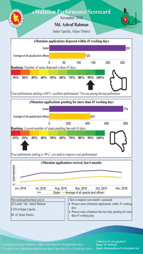
Together with the Government of Bangladesh, I designed a monthly performance scorecard addressed
to the ACL and sent to randomly selected sub-district land offices, as well as to the offices of the UNO
and the DC, the ACL’s two direct superiors. The scorecard is intended to decrease delays in applica-
tion processing for land record changes. Appendix Figure A4 presents an example of a performance
scorecard.
The scorecard evaluates the ACL’s performance using two performance indicators. The first indica-
tor is the number of applications disposed within 45 working days in the past month, where a higher
number indicates a better performance. The second indicator is the number of applications pending
beyond 45 working days at the end of the month, where a lower number indicates a better performance.
The scorecard shows both these numbers as well as the average numbers for all sub-district land offices
in the experiment. The scorecard also provides the office’s percentile ranking for each indicator, with
a short sentence reflecting the performance. Finally, to make the score easily understandable and more
salient, a thumbs-up symbol is put next to percentile rankings between the 60th and the 100th percen-
tile, while a thumbs-down symbol is put next to percentile rankings from the 0th percentile to the 40th
percentile. Two versions of the scorecard, one in English and one in Bengali, were sent out in the first
two weeks of each month with information based on the previous calendar month’s e-governance data.
Offices in the treatment group were not informed that they would receive a scorecard before the start of
the treatment, but the first scorecard was followed by a phone call to the ACL where the indicators were
explained and the ACLs could ask questions about the scorecard. The scorecards are also accompanied
by an explanatory note showing how the numbers in the scorecard are calculated and a phone number
to call to ask questions about the scorecard.
2.3.1 Additional intervention: List of peer performances
To test for peer effects, an addition was made to the scorecards for 77 randomly selected treatment
offices in September 2019, a year after the first scorecards were sent out. The purpose was to test if there
was an additional effect, beyond the effect of the scorecard, stemming from a bureaucrat’s performance
being observable to the bureaucrat’s peers at the same position in the organizational hierarchy. For a
randomly selected group of 77 offices within the offices already receiving the performance scorecards,
a list of the percentile rankings of the two performance indicators for all 77 offices was added to the
scorecard. Appendix Figure A5 shows an example of the first page of such a list. The main difference
10between receiving the typical scorecard and the scorecard with the list of performances was that for the
offices that received the list of performances, their performance was observable not just to them and their
supervisors but also to 76 of their fellow ACLs.
2.4 Randomization
Figure 2 provides a visual overview of the randomized interventions and data sources. The randomiza-
tion was done in two waves. In August 2018, 112 land offices were using the e-governance system. In
the first randomization wave, 56 of these offices were randomly chosen to receive the performance sco-
recards, while 56 were assigned to the control group.7 In April 2019, 199 additional offices had started to
use the e-governance system and a second randomization wave was carried out to increase the experi-
ment’s sample size. The second randomization wave extended the treatment to 99 new offices while 100
new offices were added to the control group.8 The additional list of peer performances was added to the
scorecard for 77 randomly selected offices receiving the scorecards in September of 2019. The scorecards
were sent out until March 2020, when the outbreak of COVID-19 caused an end to the scorecards being
sent out.
Both randomization waves were stratified by the number of applications processed within 45 wor-
king days in the two months preceding the randomization and the number of applications pending for
more than 45 working days at the end of the month preceding the randomization. For the first rand-
omization, another binary variable for being a land office where the e-governance system was fully
implemented, meaning that no applications were conducted using the traditional paper-based method,
was also used for stratification. In the second randomization, the total number of received applications
was used as a stratification variable. The randomization of offices into receiving the peer performance
list was done among the 155 offices receiving the scorecards using the same stratification variables as the
second randomization wave. For more information about the randomizations see Appendix Section B.1.
2.5 Data
I use two main data sources, administrative data from the e-governance system and data from a survey
conducted among applicants in the 112 land offices that were part of the first randomization wave. I
use the administrative data to generate the performance scorecards as well as evaluating the effects of
7 The first randomization was carried out by the author on 14 August 2018.
8 The second randomization was carried out by the author on 10 April 2019.
11the scorecards. Table 1 shows summary statistics for both data sets. This table contains all observations
from both treatment and control offices that are used in the analysis. For a discussion of the balance of
randomization, see Section 2.6.
2.5.1 Administrative data
The observations in the administrative data are at the application level. The data contains information
about in which land office the application was made, the application start date, the date it was pro-
cessed as well as the decision to accept or reject the application. The administrative data also contains
information on how large the land plot for which the change is being made is.9 The administrative data
was downloaded from the e-governance system at the beginning of each month from August 2018 until
October 2020.
For the main analysis, I use administrative data for applications from 13 August 2018, 1 month before
the start of the experiment, until 20 January 2020. From 26 March 2020 and onwards the COVID-19 out-
break in Bangladesh substantially increased processing times for land records changes as measured by
calendar days but also resulted in a large number of general holidays, increasing the difference between
calendar days and working days. At this time, the scorecard intervention was also stopped. Therefore, I
do not include applications made after 20 January 2020, 45 working days before the start of the general
holiday caused by COVID-19, in the analysis. Ending the data at this point precludes the holiday from
affecting one of the main outcomes, if the application was processed within the 45 working day time
limit or not.
I impute the processing times for the 6% of applications that have not yet been processed. The
imputed value is the mean of actual processing times that are larger than the number of working days
the application that I am imputing the processing time for has been pending.10 The data set in the
main analysis contains 1,050,924 applications from all 311 offices. Appendix Section B.2.1 provides more
information about the administrative data.
9 The full administrative data set also contains more information about the applicants, but this data is not available for
research purposes due to privacy concerns.
10 This procedure is conservative in two ways. First, it reduces any effect on processing times generated by the scorecards
since the same mean is used to impute values in both the treatment and control areas. Second, the mean used to impute
processing times in this procedure likely underestimate the time it will take to process these applications on average since it
is the mean of applications that have already been processed, which is likely to be less than the actual average time it will take
to process all applications including those currently pending. Since the point estimate of the scorecards’ effect on the share of
applications being pending is a decrease of 0.9 percentage points, using these imputed values creates a conservative estimate
of the effect of the scorecards on processing times.
122.5.2 Survey data
The survey data was collected in two rounds from applicants who applied in the 112 offices that were
part of the first wave of randomization. The sample of applicants was created by placing surveyors
outside land offices and interviewing all applicants entering the office for the purpose of a land record
change application, regardless of what stage in the application process they were at. The surveyors
stayed outside a specific office for at least two days and until they had completed at least 20 interviews.
The follow-up interview was conducted by phone approximately three months after the initial interview.
Surveyors were not informed about which offices had received the scorecards or if they were calling a
respondent from a treatment or control office.
Out of 3,696 people approached, a total of 3,370 applicants were successfully interviewed in the
first round interview outside of the land offices. Out of those interviewees, 3,018 were successfully re-
interviewed in the follow-up phone interview, resulting in a total attrition rate of 18%. The estimated
effect of the scorecards on the attrition rate was 3 percentage points and marginally statistically signi-
ficant at the 10% level. However, in Appendix Section B.2.3 I show that this differential attrition is not
sufficiently large to substantially affect the main findings from the survey data. More information about
the survey data can be found in Appendix Section B.2.2.
The initial interview focused on the details of the application, the applicant’s expectation for the
application processing time, the applicant’s willingness to pay for faster processing, as well as basic
information about the applicant. The follow-up interview focused on the outcome of the application
and the payments, above the official fee, that the applicant had made in relation to the application.
Data on bribe payments was collected using two different questions. The first question asked what
the typical bribe payment is "for a normal person like yourself." If the respondent were willing to answer
this question, the amount, whether zero or positive, was recorded as the variable typical payment. 63%
of respondents provided an answer to this question and the average response was BTD 6,731 (~USD 80)
or 1.5 months of the sample’s average per capita household expenditure.11 73% of the responses were
non-zero amounts. The second set of questions asked about each actual payment made by the applicant
to any government official or agent assisting with the application. The outcome variable reported payment
is the sum of the bribe amounts reported in each of these questions. This variable takes the value zero
when no payments were reported. Since the most common response for respondents who were not
11 Variables
are winsorized at the 99th percentile and averages are calculated using observations weighted by the inverse of
the number of observations in each office.
13willing to talk about payments that they had made was to report no payment, as opposed to stating that
they did not want to respond to the question, the average reported payment is likely an underestimate of
the actual payments. The average reported payment was BDT 1,456 (~USD 17) and 27% of respondents
provided a non-zero value. Among those reporting a non-zero amount the average amount was BDT
5,283 (~USD 63).
2.6 Balance of randomization
Appendix Table A1 shows a balance of randomization test for the two main outcome variables from the
administrative data, the fraction of applications processed within 45 working days and the average pro-
cessing time. The data used is restricted to applications made at least 45 working days before the start
of the experiment. Applications that were not processed by the start of the experiment were assigned an
imputed processing time, using the imputation procedure described in Section 2.5.1. There are no sta-
tistically significant differences between scorecard and control offices before the start of the experiment.
This is expected given that the random treatment assignment.12
Appendix Table A2 shows that the scorecards did not affect the composition of applicants or appli-
cations in the survey data. This is not a traditional balance of randomization table, since the treatment
may have affected which applicants decided to apply and what type of applications to make. However,
I do not find any evidence for such changes in behavior. I find no statistically significant difference in
the age or income of the applicants, or in the size or value of the land that the applications are for. Furt-
hermore, there are no substantial differences between the stages that the applications are in at the time
of the first interview. When using the regression specification from Equation 1 on this data, the effect of
the scorecards is not significant at the 5% for any of the outcome variables, and significant at the 10%
level only for land value.13
2.7 Additional intervention: Providing information to applicants
Together with the in-person survey, an intervention providing additional information to applicants was
also carried out on randomly selected days in each office where the survey took place. The motivation
12 Using the empirical strategy described in Section 3.1 on the data from before the start of the experiment also generates
statistically insignificant estimates of the effect of the treatment on the outcome variables. Furthermore, an F-test of joint signi-
ficance for the explanatory power of the outcome variables on the treatment variable cannot reject the null of no explanatory
power (p-value: 0.69).
13 F-tests of joint significance for the explanatory power of the outcome variables on the treatment variable cannot reject the
null of no explanatory power (p-value: 0.73).
14behind this intervention was to ensure applicants knew about the improvements in processing times.
While it is likely that this information would eventually have spread, in the short-term, information
about changes to bureaucrat behavior may not yet have disseminated. If the applicants are not aware
of the improvements in processing times, the long-term effects on bribe payments may not yet have
been realized. To speed-up the dissemination process, and potentially reach the long-term effect of the
scorecards faster, the surveyors randomly provided information about increased processing speeds on
half of the days that the in-person survey was conducted. The surveyors used an information pamphlet
to inform applicants that the median processing time for all land offices had been substantially reduced
over the past six months and that a new e-governance system had been installed. The information the
surveyors provided was the same in both treatment and control offices. The scorecard intervention
was not mentioned to applicants. Appendix Figure A6 shows an English translation of the information
pamphlet. I will analyze the results of the intervention when testing the predictions of models connecting
processing times and corruption in Section 5.
3 Empirical Strategy
3.1 Empirical strategy: Overall effects
To estimate the effects of the scorecards, I use the following regression specification:
Outcomeait = α + βTreatmenti + Stratai + Montht + ε ait (1)
Where Outcomeait is an outcome for application a, in land office i, made in calendar month t. Stratai
are randomization strata fixed effects. Since no randomization strata overlap the two randomization
waves, these fixed effects also control for randomization wave fixed effects. Montht are fixed effects for
the month the application was made. In the survey data, all continuous variables are winsorized at the
99th percentile.14 Standard errors are clustered at the land office level resulting in 311 clusters in the
administrative data and 112 clusters in the survey data. Each observation is weighted by the inverse of
the number of observations in land office i. Therefore, the estimated effect is the average effect of the
scorecard on a land office, the level at which the treatment was assigned. The weighting also improves
14 In the survey data, the application month variable is winsorized at November 2018, so that all application dates before
November 2018 take the value of November 2018. A separate dummy variable controls for missing start date values.
15the estimates’ precision by making each cluster have equal weight in the analysis.15
3.2 Empirical strategy: Heterogeneous effects
To better understand the mechanisms behind the overall effects, I separate offices by their baseline per-
formance and estimate the effect of the scorecards separately for offices performing above and below
the median at baseline.16 I calculate each office’s baseline performance based on the average of the two
percentile rankings at the time of the first scorecard. One ranking is based on the number of applications
disposed within 45 working days, while the other is based on the number of applications pending for
more than 45 working days. For offices in the treatment group, these are the actual rankings shown on
the first scorecard, while for the control group, the rankings were not shown to the bureaucrats. I then
separate all offices into over-performers, that were above the median average ranking at baseline, and
under-performers, that were below the median average ranking at baseline.17 Since the classification of
offices only uses data from before the first scorecard was delivered, it is not affected by the treatment.
I use the following regression specification to estimate the effect of the scorecards on the two types
of offices separately:
y ait =α + β 1 Treatmenti × Overper f ormi + β 2 Treatmenti × Underper f ormi +
γOverper f ormi + Stratumi + Montht + ε ait (2)
Where β 1 is the estimated effect of the scorecards for offices over-performing at baseline, β 2 is the effect
for offices under-performing at baseline, and γ is the difference between over-performing and under-
performing offices in the control group.18 As in the estimation of the overall effects, standard errors
15 For a discussion of why weighting observations by the inverse of the number of observations in a cluster improves pre-
cision see: https://blogs.worldbank.org/impactevaluations/different-sized-baskets-fruit-how-unequally-sized-clusters-can-
lead-your-power
16 Heterogeneity in the effects of performance information provision between high and low performers has been recorded
in several settings (e.g., Allcott, 2011; Dodge et al., 2018; Ashraf, 2019; Barrera-Osorio, Gonzalez, Lagos, and Deming, 2020).
This was the only heterogeneity test based on office characteristics specified in the pre-analysis plan. The two other pre-
specified tests for heterogeneity were based on the date of application and the application processing time. The estimates of
heterogeneity in the effects along those dimensions are shown in Figure 4 and Appendix Table A3, respectively.
17 I classify offices in the first randomization wave into over- and under-performers by comparing them to the median perfor-
mance among these 112 offices at the time of their first scorecard (September 2018). For the offices in the second randomization
wave, I compare them to the median performance of all 311 offices in the experiment at the time of their first scorecard (April
2019). This ensures that the over- and under-performer classification corresponds to if the content in the first scorecards was
above or below the median of comparison groups at the time.
18 To test the hypothesis that the treatment had the same effect on offices over-performing and under-performing at baseline,
I use a similar regression but where the first treatment variable is not interacted with the dummy variable for if the office over-
performed at baseline. I then test the hypothesis that the coefficient on the treatment variable interacted with with the dummy
variable for if the office was under-performing at baseline is zero. This test’s p-value is reported as "P-value sub-group diff." in
the regression tables reporting the heterogeneous effects.
16are clustered at the land office level and the regressions are weighted by the inverse of the number of
observations in land office i.
3.3 Analysis of additional experiments and potential interactions
The two additional randomized interventions, the addition of peer performance lists and the information
intervention to applicants, are not included in the main specification as these interventions are not the
main treatments being evaluated. For the two main outcomes, delays and bribe payments, the full
specifications, including the scorecard treatment, the additional randomization, and the interaction, can
be found in Tables 3 and A4. These tables show that neither of the two additional experiments have
substantial interactions with the scorecard treatments, validating the approach to analyze the scorecard
treatment separately as outlined in Equations 1 and 2.
4 Results: Effects on Processing Times, Bribes and Visits by Applicants
This Section shows the estimates of the effects of the scorecards on processing times, visits to land offices
made by applicants, and bribes. Appendix Section C.3 investigates potential unintended consequences
of the scorecards on bureaucrats’ behavior and does not find evidence for any large unintended conse-
quences.
4.1 Effect on processing times
Table 2 shows that the scorecards increased the applications processed within the government time li-
mit and improved processing times overall. Each column presents the result of a regression using the
specification in Equation 1. Column (1) shows the estimated effect of the scorecards on a binary variable
indicating if the application was processed within the 45 working day time limit or not. The scorecards
increased the fraction of applications processed within the 45 working day limit by 6 percentage points
or, equivalently, 11%. Column (2) shows the estimated effect on the Inverse Hyperbolic Sine (IHS) trans-
formation of the number of working days it took to process the application.19 Column (2) estimates
that the scorecards reduced the processing time by 13%.20 In the data, 6% of the applications are not
19 The IHS transformation is used instead of the natural logarithm since 0.3% of the applications were processed on the same
day as they were made and therefore have a processing time of zero working days. The results are virtually identical when
dropping the applications taking zero days to process and using the natural logarithm transformation.
20 The exact effect is 13 IHS points, which are approximately equivalent to log points. A 13 log point decrease is equivalent to
a 12% decrease, but for simplicity, I will describe IHS points changes as percentage changes throughout the paper. Appendix
Table A6 shows that the result is similar when dropping the observations with processing times of zero working days and
17yet processed, and for the analysis in Column (2) I have assigned imputed processing times for these
applications, using the imputation procedure described in Section 2.5.1. Appendix Table A5 shows that
the results are robust to different imputation techniques. In Appendix Table A6 I test the robustness of
the result to using different functional form assumptions for the relationship between the scorecards and
processing times.
For Column (3), I create an Inverse Covariance Weighted (ICW) index of the two outcomes used
in Columns (1) and (2).21 The estimated effect of the scorecards on the ICW index is 0.13 standard
deviations and statistically significant. In Appendix Table A7 I test the robustness of this result with
various alternative specifications. All alternative specification estimates are of the same sign and similar
magnitude as the main estimate, but some of them are not statistically significant. Appendix Table A8
shows the effects, estimated at the office by month level, on the number of applications processed within
45 working days, the number of applications pending beyond 45 working days as well as those figures
corresponding percentile rankings. The point estimates suggest that the scorecards improved all four of
these outcome variables but the effects are not statistically significant.
4.1.1 Effect over time
Figures 3 and 4 show that there is no pattern of the effect declining over time, although the size of the ef-
fect varies between different time periods. Figure 3 shows the fraction of applications processed within
the 45 working day limit over time for the treatment and control group separately. The first dashed
vertical line indicates the date 45 working days before first scorecards. The second dashed vertical line
indicates the date of the first scorecards. Applications made between the first and second vertical lines
may have been affected by the scorecards if they were not processed before the first scorecard was sent
out. Starting for applications made a few days before the first scorecards, we see a divergence between
the treatment and control group. The treatment group increased the fraction of applications that were
processed within the 45 working days time limit, relative to the control group. With a few short excep-
tions, the treatment offices continue to have a higher fraction of applications processed within the time
limit relative to the control offices until the end of the experiment. The data for the offices in the second
using the natural logarithm transformation.
21 The ICW matrix follows the algorithm suggested by Anderson (2008) and is designed to summarize several outcome
variables into one index that, for the control group, has a mean of zero and a standard deviation of one. Since there are only
two outcome variables in Table 2, the ICW index is equivalent to summing the standard deviations away from the control
group mean of the two variables and rescaling the index to have a standard deviation of one in the control group. However, in
tables with more than two outcome variables, the components are weighted differently to maximize information captured by
the ICW index.
18randomization wave ends earlier relative to the start of the experiment. The third vertical dashed line
marks where the data from the second randomization wave ends. To the right of this line, the graph only
contains data from the offices in the first randomization wave. Appendix Figure A7 shows the time lines
for the two randomization waves separately.
Figure 4 shows the results of applying the regression specification from Equation 1 to applications
made in the first, second, and last third of the experiment period. The outcome variable is the ICW Index
from Column (3) of Table 2. When I split up the sample, the estimates lose some precision, but it is clear
from the graph that there is no pattern of a continuous decline of the effect over time.
4.1.2 Effect on the distribution of processing times
Figure 5 shows two overlaid histograms, one for the distribution of processing times in the treatment
group and one for the distribution in the control group. The figure only includes applications that have
already been processed and processing times are top coded at 200 working days. In the treatment offices,
more applications were processed within the 45 working day time limit. The effect is relatively evenly
spread over the whole span from 0 to 45 working days, with only a minor bunching just before the 45
working day limit. This is to be expected given that the process to approve an application is relatively
long and depends on several individuals, as described in Section 2.1. This means that even if the ACL
targets a 45 working day processing time, there will be a considerable spread around this target. Because
of this, the ACLs may target a processing time lower than 45 working days. The figure also shows that
the processing times that are reduced in frequency by the scorecards are in the whole span from 55
working days and up. This is also reasonable given that the scorecards emphasized both processing
applications within the 45 working day limit and reducing the number of applications pending beyond
45 working days. Overall the spread of the effect in the distribution of processing times alleviates the
concern that ACLs are "gaming" the scorecards by only speeding up the processing of applications that
would otherwise have been processed within a few working days outside of the time limit.
4.2 Mechanisms for the effect on processing times
The scorecards increase the information the bureaucrats and the bureaucrats’ supervisors have about
the performance of the bureaucrat. This could improve performance through two main channels. First,
the supervisors may improve the incentive structures the bureaucrat is facing by facilitating better pro-
motions and more attractive postings for those bureaucrats with good scorecards, or more generally,
19bureaucrats with a good overall reputation of which the scorecards are a part. This is an example of
the widely studied mechanism of increased information enabling better contracts that improve output
(Holmström, 1979). It is also possible that bureaucrats care about their supervisors receiving information
about them for other reasons, such as the shaming effect of having a negative performance being shown
to a superior.
Second, bureaucrats may change their behavior due to receiving the scorecards themselves. For bu-
reaucrats, receiving information about their delays each month may increase this information’s salience,
causing it to be more important for their personal sense of shame or pride in their work.22 Since the sco-
recards were sent to both bureaucrats and their supervisors, I cannot separately estimate the importance
of these two mechanisms and I refer to them collectively as reputational concerns.
In addition to the two mechanisms above, it is also possible that information flows between bureau-
crats at the same level in the organizational hierarchy create an additional incentive for improved per-
formance through peer effects (Mas and Moretti, 2009; Bandiera, Barankay, and Rasul, 2010; Cornelissen
et al., 2017).23 I estimate the magnitude of such a peer effect, above and beyond the effect of the score-
card, by sending information about other offices’ performance within a randomly selected sub-group of
the offices receiving scorecards, as described in Section 2.3.1.
Table 3 shows the effect of the peer performance list intervention on processing times. Sharing the
performance information of a bureaucrat with other bureaucrats does not meaningfully improve pro-
cessing times beyond the effect of the performance scorecards. Column (1) of Table 3 shows that the
estimated effect on the fraction of applications processed within the 45 working day time limit is posi-
tive but close to zero. Column (2) shows that the effect on overall processing times is negative but also
close to zero.24
22 Effects from simply being informed of one’s own performance have been found for energy conservation (Allcott, 2011).
On the other hand, the effects of such information provision in private organizations have been mixed, with several papers
showing that even the direction of the effect depends on the specific circumstances (Blader, Gartenberg, and Prat, 2020; Ashraf,
2019).
23 In addition to the context of job performance, effects of sharing information about behavior to others have shown to
improve socially desirable behaviors such as voting (Gerber, Green, and Larimer, 2008) and paying taxes (Bø, Slemrod, and
Thoresen, 2015; Perez-Truglia and Troiano, 2018).
24 Columns (3) and (4) of Table 3 use the full data set and estimate the effect of the scorecard and the peer performance
list simultaneously. This is done using a dummy variable for the peer performance list treatment that takes the value of one
for applications made in offices receiving the peer performance lists, made later than one calendar month before the first
performance list was sent out. When estimating the effects of the scorecards without the effect of the performance list, the
point estimates are similar to the effect in the main estimate but only statistically significant at the 10% level. This shows that
the effect of the scorecards is not driven by the inclusion of the peer performance list.
20You can also read