Integrated Bayesian risk analysis of ecosystem management in the Gulf of Finland, the Baltic Sea - How to do it?
←
→
Page content transcription
If your browser does not render page correctly, please read the page content below
Not to be cited without prior reference to the author                                        ICES CM 2012/I:04

Integrated Bayesian risk analysis of ecosystem management in the Gulf of Finland, the Baltic Sea
– How to do it?
Inari Helle, Jarno Vanhatalo, Mika Rahikainen, Samu Mäntyniemi & Sakari Kuikka

Abstract

Human activities may have devastating effects on marine and freshwater ecosystems. The negative impacts
can develop gradually (e.g. increased nutrient runoff resulting to eutrophication) or they can be abrupt and
catastrophic (e.g. spills of harmful substances). Usually both the frequency and impacts of these events are
difficult to predict and scientific uncertainties are high. In addition, ecosystems are often threatened not
only by a single factor, but instead by multiple stressors at the same time. Due to this complexity it is
difficult e.g. for decision-makers to realistically evaluate the effects of alternative management options. In
this paper we demonstrate how to create a probabilistic decision model to assess the effects of several risk
factors on different components of the ecosystem in the Gulf of Finland, the easternmost part of the Baltic
Sea. The risk elements considered are eutrophication, oil spills and harvesting. With the model one can
estimate the effects of these factors on some example species and water quality variables in the Gulf of
Finland. The general model is a Bayesian network, which uses various inputs, e.g. the results produced with
3D ecosystem models and stochastic population dynamics simulation models. Although we use the Gulf of
Finland as a case study, the methodology is applicable also to other areas facing multiple risks. The model
can also be developed further to encompass the costs and benefits of the alternative management actions.

Keywords: Bayesian networks, Gulf of Finland, environmental management, multiple risks

Contact author: Inari Helle, Fisheries and Environmental Management Group (FEM), Department of
Environmental Sciences, University of Helsinki, P.O. Box 65, FI-00014 University of Helsinki, Finland, tel: +358
50 311 2574, email: inari.helle@helsinki.fi

Jarno Vanhatalo, Fisheries and Environmental Management Group (FEM), Department of Environmental
Sciences, University of Helsinki, P.O. Box 65, FI-00014 University of Helsinki, Finland, tel: +358 50 317 5494,
email: jarno.vanhatalo@helsinki.fi

Mika Rahikainen, Fisheries and Environmental Management Group (FEM), Department of Environmental
Sciences, University of Helsinki, P.O. Box 65, FI-00014 University of Helsinki, Finland, tel: +358 50 311 2472,
email: mika.rahikainen@helsinki.fi

Samu Mäntyniemi, Fisheries and Environmental Management Group (FEM), Department of Environmental
Sciences, University of Helsinki, P.O. Box 65, FI-00014 University of Helsinki, Finland, tel: +358 50 415 1098,
email: samu.mantyniemi@helsinki.fi

Sakari Kuikka, Fisheries and Environmental Management Group (FEM), Department of Environmental
Sciences, University of Helsinki, P.O. Box 65, FI-00014 University of Helsinki, Finland, tel: +358 50 330 9233,
email: sakari.kuikka@helsinki.fi
1. Introduction

Throughout the world, marine and freshwater ecosystems are impacted by human activities that may lead
to severe environmental problems. The negative impacts can develop gradually (e.g. increased nutrient
runoff resulting to eutrophication) or they can be abrupt and catastrophic-like (e.g. spills of harmful
substances). Both of these are probabilistic in nature, as the impacts of stressing factors are not known for
sure, and especially in the case of catastrophes, also the frequency of events is difficult to predict.

The management of these problems is challenging for several reasons. First, ecosystems usually embody
complex interactions and e.g. feedback loops, and spatial and temporal natural variability is usually high.
Both the causalities and natural variability create uncertainties, which should be quantified as a part of any
management process. Second, there is seldom only one potential threat to be considered, which means
that the combined effect of multiple risk factors should be evaluated and the management actions planned
in an integrative manner instead of examining them one by one. Third, major uncertainties are present not
only within ecosystems but also on the human side of the management, and it is difficult to predict the
behavior of people, i.e. their reactions and commitment to management decisions. It is thus evident that to
be able to evaluate beforehand the effects of different management actions there is a need for models that
take into account above-mentioned matters.

The Baltic Sea, a semi-enclosed brackish water sea situating in the northern Europe, is facing multiple
human-induced environmental problems like severe eutrophication (HELCOM 2009), intense maritime
traffic increasing the risk of oil spills (HELCOM 2010a) and overharvesting (HELCOM 2007a). It has been
estimated that none of the open sea areas in the Baltic Sea can be classified as having a “good ecosystem
health status” and the situation with the coastal areas is almost equally severe (HELCOM 2010b). At the
moment, the protection of the Baltic Sea environment is based on the common legislation of the European
Union (e.g. the Water Framework Directive (WFD) for coastal waters), international conventions like the
Helsinki Convention and programs based on the conventions (e.g. the Baltic Sea Action Plan, BSAP) and
national legislations of the coastal states.

In this paper we present a probabilistic decision model that can be used to evaluate the effectiveness of
different management actions directed to improve the status of the Gulf of Finland (GoF), the easternmost
part of the Baltic Sea. The risk elements considered in the model include eutrophication, oil spills and
harvesting. With the model one can review the effects of these factors on two example species and water
quality variables within the GoF. The model is a Bayesian network, which uses various kinds of inputs, e.g.
results produced with 3D ecosystem models as well as Bayesian population dynamics simulation models.

The main aim of the paper is to demonstrate, how to create a decision model that 1) integrates different
risk elements simultaneously, 2) takes uncertainty into account in a coherent manner, and 3) is user-
friendly and whose results are easy to interpret.

2. Methods

2.1. Study area: the Gulf of Finland

The Gulf of Finland (GoF) is a relative shallow, elongated estuary in the northern part of the Baltic Sea
surrounded by Finland, Estonia and Russia (Fig. 1). The average depth of the gulf is only 37 m, and thus its
water volume is small, only 5 % of the volume of the whole Baltic Sea (Alenius et al. 1998). This makes the
GoF sensitive to degrading activities within the drainage area. The salinity is low (0–7 ‰) compared to
oceans, and it is regulated by the intrusion of saline water from the Baltic Sea main basin and the major
inflow of fresh water from the River Neva, the biggest river running into the Baltic Sea. In winter, the GoF
may freeze entirely, and the ice cover period lasts typically 43–135 days (Seinä & Peltola 1991). Due to
northern location, relatively short geological history, and low water salinity, the biota of the GoF is a
mixture of marine and freshwater species capable of coping with low salinities and ice-cover in wintertime.
The GoF is also an important migratory route for arctic birds, and it harbors numerous conservation areas
(Furman et al. 1998, HELCOM 1996).

Today, the GoF is suffering from severe eutrophication as the nutrient loads relative to the surface area
have been 2–3 times the average of the Baltic Sea (Pitkänen et al. 2001). This has had drastic
consequences, e.g. extensive bottom areas are classified hypoxic or anoxic yearly (Hansson et al. 2011). The
GoF is also one of the most densely operated sea areas in the world. Especially oil transportation has
increased during the past 15 years as Russia has constructed new terminals and modernized the old ones.
In 2008, already half of the oil exported from Russia was transported via the GoF (Hietala 2008).

Figure 1. Gulf of Finland

2.2. Bayesian networks

Bayesian networks (BNs) are graphical models, which describe probabilistic relationships between variables
within a system. Formally a BN is a directed acyclic graph (DAG), whose structure expresses the current
understanding of the problem of interest and cause-effect relationships within it.

In a BN, random variables are usually represented by rounded nodes and dependencies between the
variables by arrows. A node that has one or more incoming arrows is called a “child”, whereas a node
having outgoing arrows is called a “parent”. As BNs are based on probabilistic rather than deterministic
approach, each variable has one or more mutually exclusive states, over which a probability distribution is
assigned. If a node has no incoming arrows (i.e. it is not dependent on any other variables), it has a
marginal probability distribution, whereas a node having one or more incoming arrows (i.e. it is dependent
on other variables) has a conditional probability distribution describing the probability of each state of the
child node, conditioned on every possible combination of the states of the parent nodes. A more detailed
description of the methodology related to BNs can be found e.g. from Jensen (2001).

By adding decision and utility nodes to BNs they can be extended to Bayesian influence diagrams (BIDs),
which improves their use as a decision support tool. By choosing one decision option (or combinations of
decisions in case of several decision nodes) at a time one can examine the consequences of planned
management actions, as the information is propagated through the network.

Several quantitative and/or qualitative techniques can be used to quantify marginal and conditional
probability distributions within a network; these include e.g. observed data, simulation results and expert
knowledge (Uusitalo 2007). This feature makes BNs a flexible way to integrate data and knowledge from
different sources and disciplines. As this need is evident in many environmental management problems,
BNs are increasingly used e.g. in fisheries (e.g. Kuikka et al. 1999, Levontin et al. 2011) and water resources
management (e.g. Varis et al. 1990, Bromley et al. 2005, Molina et al. 2010).
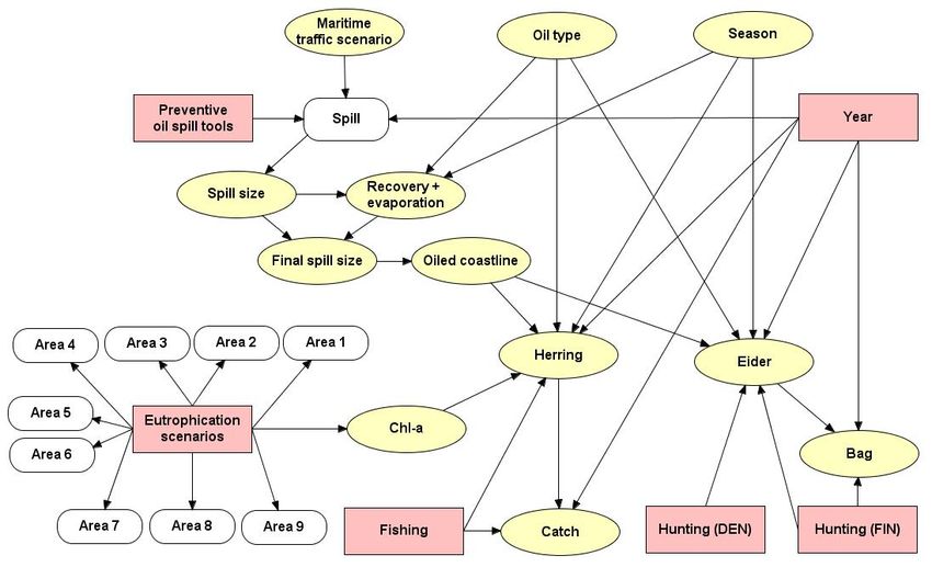
3. Integrative model

The integrative model developed in this study considers three risk factors present in the GoF:
eutrophication, oil spills and harvesting. The structure of the model is presented in Fig. 2. The combined
effects of these factors can be studied on two species: Baltic herring (Clupea harengus membras) and
common eider (Somateria mollissima). Although both species are still abundant in the GoF, their
populations have encountered major changes in recent decades, as e.g. the growth rate of Baltic herring in
the GoF declined dramatically in 1985–2000 (Rönkkönen et al. 2004), and the wintering stock of the
common eiders declined by 40–50 % in the Baltic Sea in 1990–2000 (Desholm et al. 2002). In Finland, the
status of common eider was changed to “Near threatened” from “Least concern” in the recent IUCN
assessment (Rassi et al. 2010).

The model output can be explored in three occasions, i.e. years 2015, 2021 and 2027 (decision variable
“Time period”). These occasions are based on the management cycles of the EU’s Water Framework
Directive (WFD) (European Parliament and Council 2000).

Figure 2. Structure of the intergrative BN. Ellipses = random variables, squares = decision variables, rounded squares =
submodels. See text for more detailed description of the variables.

3.1. Eutrophication

The eutrophication part of the integrative BN model can be used to assess the probability to reach the
water quality targets set by the WFD or the Helsinki Commission (HELCOM). In addition, it provides an
estimate on the average chlorophyll-a concentration within 10 km radius from the coastline. The
parameters of BN model were estimated with the EIA-SYKE 3D ecosystem model (Kiirikki et al. 2001), which
calculates e.g. the chlorophyll-a values given the nutrient loads entering the GoF.

Four water quality variables are assessed with respect to the aims of the WFD and HELCOM Baltic Sea
Action Plan: nitrogen, phosphorus, chlorophyll-a and Secchi depth. However, there are some differences
between the two approaches, as e.g. the WFD considers total nutrients whereas HELCOM is interested in
inorganic nutrients. Further, the WFD is applied in coastal areas, whereas HELCOM operates in open sea
areas. In order to be able to see simultaneously how aims of policies can be achieved in different areas,
the GoF was divided in 9 subareas, each of which has its own submodel in the integrative model (see Fig. 2):
areas 1–4 represent Finnish coastal waters, 5–6 Estonian coastal waters and 7–9 open sea areas. The
Finnish and Estonian coastal waters (1–6) are delineated according to the national implementations of the
WFD, and the open sea areas (7–9) according to the similarity analysis conducted in the (former) Finnish
Institute of Marine Research (see Lindén et al. 2008).

The discretization of the water quality variables is based on the class boundaries set by the WFD and target
values set by HELCOM. According to the WFD, each variable has five classes that correspond states “High”,
“Good”, “Moderate”, “Poor” and “Bad”, whereas HELCOM defines one target value for each variable. The
WFD class boundaries for Finland are reported in Vuori et al. (2009) and for Estonia in Anonymous (2009).

Nutrient reductions scenarios

The decisions related to eutrophication (decision node “Eutrophication scenarios”) represent 6 different
nutrient loading scenarios for Finland, Estonia and Russia: 1) Baseline (BSL) scenario for all countries, 2) the
full implementation of the Baltic Sea Action Plan (BSAP) targets for all countries, 3) the 50 %
implementation of BSAP targets for all countries (BSAP50), and 4–6) different reduction scenarios for
Finland designed according to the national Water Protection Policy Outlines for 2015 (Rekolainen et al.
2006) and BSL for Estonia and Russia (FIN1–FIN3).

For Finland, the BSL was based on monthly mean values of nutrient loading in riverine discharges and
coastal point sources in 2000–2004. For Estonia, BSL was based on the mean monthly values in 2000–2003
(data provided by the Estonian Marine Institute, University of Tartu), and for Russia on the loadings in 2000
(Pitkänen & Tallberg 2007).

The BSAP calls for clear reductions in nutrient loadings within the Baltic Sea. E.g. in the GoF, there should
be a reduction of 2 000 tons on phosphorus load and 6 000 tons on nitrogen load (HELCOM 2007b). In
scenarios 2 and 3 this total reduction, or 50 % of it, was supposed to be implemented evenly within three
coastal countries, i.e. a same percentual cut was carried out for every point source and riverine load.
However, for the city of St. Petersburg (Russia) situating in the easternmost tip of the GoF, the loading
values representing the year 2011 were used, as Russia has already exceeded its BSAP targets due to the
large-scale investments in the wastewater treatment plants of the city.

Modeling of water quality

The modeling of the water quality was done in two phases. The preliminary modeling was carried out with
the EIA-SYKE 3D ecosystem model (Kiirikki et al. 2001), which simulates the weekly averages of dissolved
nutrients (N, P) and algal biomass under different loading scenarios for a grid cells of 5x5 km across the
GoF. The model is calibrated for years 2000–2004 with data from the same time period. The total nutrients
(used in WFD approach) were estimated from the modeled dissolved nutrients, and Secchi depth was
calculated based on modeled chlorophyll-a concentrations.

However, as the EIA-SYKE 3D ecosystem model is deterministic, a statistical correction for simulator
predictions was needed before the simulation results could be used in our probabilistic model. Statistical
correction of a deterministic simulator prediction, based on spatio-temporal or dynamic state-space
models, has previously been used e.g. in weather forecasting and climate models (Fuentas & Raftery 2005,
Berrocal et al. 2009).

We followed Berrocal et al. (2009) and constructed a following statistical correction for the simulator. Let f
represent the unobserved true concentration of a water quality variable and let x be the simulator
prediction of the same variable. The simulator prediction is assumed to be related to the true
concentration as f = a + bx, where a and b are spatially and temporally varying additive and multiplicative
bias terms. The training data are assumed to be independently and identically Gaussian distributed with
mean f. The bias terms are given Gaussian process priors and their posterior distributions are evaluated by
conditioning on the simulator predictions for and calibration data from 2000–2004. After the posterior
distributions of a and b are evaluated the future prediction is conducted. A more detailed description of the
work can be found from Vanhatalo et al. (submitted manuscript).
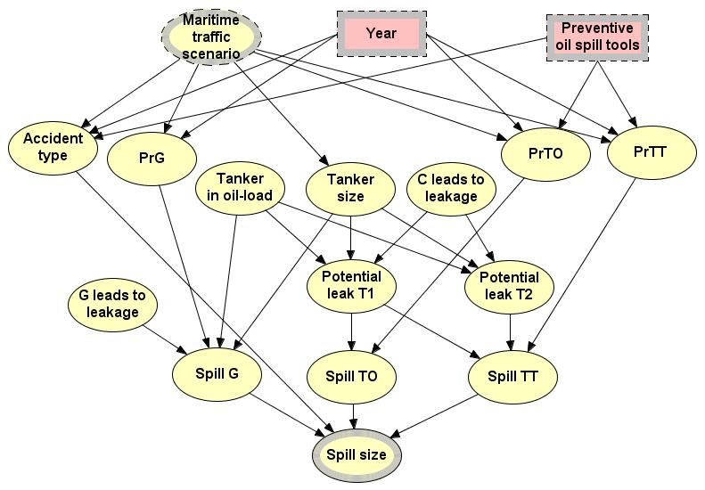
3.2. Oil spills

The oil accident part of the integrative BN describes the probability of tanker accidents and subsequent oil
spills within the GoF.

Decision variables related to oil accidents

The management options (decision node “Preventive oil spill tools”) related to the probability of oil
accidents include VTS (Vessel Traffic Service) alarm system, two revisions concerning pilot regulation and
the combinations of them. The development of these factors has been ranked as the most effective
measures to prevent oil accident in the GoF (Kuronen & Tapaninen 2010). The VTS alarm system would give
an alarm to the traffic controllers at the VTS centers, if two or more ships are on a collision course with
each other. The options related to piloting regulation include extended piloting obligations (local pilot
mandatory in all areas in the GoF), and English as an official piloting language in addition to Finnish and
Swedish. Lehikoinen et al. (manuscript) provide more information about the management options related
to oil spills.

Random variables related to oil accidents

The random variables in the oil spill part of the integrative BN model include variables related to maritime
traffic, tankers as well as timing of the accidents (see also Appendix 1).

The variable “Maritime traffic scenario” describes three maritime traffic scenarios for the future, more
specifically for year 2015. By 2015, Russia should have completed the constructions of the new oil pipeline
system (BPS-2) coming from the Eastern Russia and the new terminal in Ust-Luga, located in the south-
western coast of the GoF. The scenarios are based on economic, industrial and transportation trends in
Finland, Estonia and Russia as well as in the EU and on a global scale (Kuronen et al. 2009). The probabilities
for the scenarios were assigned by four maritime experts (Lehikoinen et al., manuscript), whose separate
judgments were integrated to form a single probability distribution.

The variable “Season” has three states, i.e. spring (March–May), summer (June–August) and autumn
(September–November). The winter months were excluded from the study, as it is extremely challenging to
predict the movement of oil in ice conditions. “Oil type” describes the type of oil transported in the GoF.
The variable has three states, i.e. light, medium and heavy oil.

The size of the spill is calculated within a separate sub-model “Spill” (Fig. 3), which estimates the probability
of tanker accidents and the volume of subsequent spills.

Three types of accidents are considered in the sub-model: groundings of tankers, collisions between two
tankers (TT) and collisions between a tanker and other vessel (TO). The probabilities of a certain number of
groundings and collisions (“PrG”, “PrTT” and “PrTO”) within a fixed time interval (i.e. from 2005 to 2015,
2021 and 2027) were estimated with Poisson distribution after having calculated the expected number of
accidents per season given different maritime traffic densities. With collisions, the calculation was
performed by using a method based on geometrical collision probability and a separate BN model
describing collision causation (Hänninen et al. 2011). The expected number of groundings (“PrG”) was
based on the HELCOM statistics for years 2004–2009 (http://maps.helcom.fi/), as there are no reliable
models describing the number of groundings in the GoF for the time being. The accident probabilities were
also used to calculate the probability distribution for the type of the accident (“Accident type”).

The variable “Tanker size” describes the size distribution of tankers in the GoF, which is dependent on
maritime traffic scenario. “Tanker in oil-load” describes the probability of a tanker to be loaded with oil.
The probability distribution was created by expert judgment. As it is not evident that groundings or
collisions of tankers result in an oil spill, the uncertainty related to this is described with variables “G leads
to leakage” and “C leads to leakage”, respectively. For groundings, the distribution was based on IMO
(2002). In respect of collisions, the probability distribution was derived from Lehikoinen et al. (manuscript),
who used eight different models to estimate the probability of leakage. In this study, the results of these
separate models were integrated to produce a single probability distribution.

All four variables presented above affect the size of the subsequent oil spill. With regard the collisions, the
spill can result from one or two tankers (“Potential leak: TO” and “Potential leak: TT”). The probability
distribution of the final spill size is expressed with the variable “Spill size”, which takes into account both
groundings and collisions.

Figure 3. Submodel “Spill” describing oil accidents in the GoF. Ellipses = random variables, squares = decision variables.
The grey border in the variables indicates inputs/outputs. See text for more detailed description of the variables.

After an oil spill, oil combating plays a major role in minimizing ecological impacts of the spill. In the Baltic
Sea, oil combating is based on mechanical recovery. In Finland, there are 15 oil combating vessels capable
of recovering oil independently. Also evaporation of oil diminishes the amount of oil in the ecosystem. The
effect of these two factors is presented with the variable “Recovery + evaporation”, the probability
distribution of which is based on the work presented in Luoma (2010). As mechanical recovery as well as
evaporation is affected e.g. by weather conditions like wind and wave height as well as the type of oil
spilled, the variable is dependent on “Season” and “Oil type”. The final amount of oil after recovery and
evaporation is presented with the variable “Final spill size”.

Random variables related to the spreading of oil and subsequent ecological effects

In the integrative BN model, the estimation of ecological effects of oil spills is based on the length of the
polluted coastline (variable “Oiled coastline”). In order to produce probability distributions for the variable,
we constructed a linear model that describes the relationship between the length of polluted coastal line
and oil spill volume and distance to shore. We conducted a Bayesian analysis by giving a zero mean
Gaussian prior for the weights of the linear model and solving their posterior, after which we were able to
evaluate the posterior predictive distribution of the length of the polluted coastal line conditional to the oil
spill volume and distance to shore. We evaluated the probability that the length of the oiled coastline falls
on a certain interval (0–10, 10–50, 50–100, 100–300, 300–600 and 600–1000 km) for 6 spill size intervals
(0–500, 500–1000, 1000–5000, 5000–15000, 15000–30000, 30000–200000 t). The data used in the analysis
comprise of 74 oil accidents on open sea (accidents on areas with ice cover were excluded from the study)
collected from literature.

The information about the length of the polluted shoreline, season and the type of spilled oil was used to
include the negative effects of spills, i.e. oil-induced mortality, in the simulation models describing the
population dynamics of the Baltic herring and common eider. The effects were derived from Lecklin et al.
(2011), who modeled the effects of oil spills on common species living in the GoF. As Lecklin et al. (2011)
used species groups instead of single species, the groups “Pelagic fish” and “Ducks” were used when
estimating the effects on juvenile and adult herring and common eider, respectively. However, as male
common eiders start their migration away from the breeding sites in the GoF already in June, and females
and juveniles usually leave the GoF in early autumn, the oil-induced mortality of eiders in autumn was set
to the lowest class.

3.3. Harvesting

The harvesting part of the model comprises the harvest decisions related to Baltic herring and common
eider. The decisions were alternative harvest mortality rates.

For Baltic herring, the harvest decisions represent fishing efforts that can be considerably lower or higher
than the estimated harvest rate in 2004, be on the same level, or match the harvest rate which is estimated
to produce the long term maximum sustainable yield (Fmsy) for the Baltic Sea Main Basin (subdivisions 25–
29 and 32 (excluding Gulf of Riga) herring stock (ICES Advice 2011). The alternative harvest efforts are
presented in Table 1.

As common eiders breeding in the GoF are harvested in their breeding grounds as well as in their wintering
areas in the Danish sea area, three harvesting options for both country, i.e. Finland and Denmark, were
included in the model: 1) the total closure of hunting, 2) Business-as-usual (BAU) harvesting, and 3) the
maximum harvesting rate of recent years (2000–2004).

Table 1. The herring fishery management options and their impact on the harvest rate.

Multiplier for fishing mortality rate     Interpretation
0.01                                      No fishing
0.5                                       Half of the harvest rate in the reference year 2004 (F 0.068).
1                                         Business-as-usual, i.e. the harvest rate in 2004 (F 0.137).
1.171728                                  Fmsy = 0.16 of the Baltic Sea herring stock.
2                                         Double harvest rate (F 0.273) compared to 2004.
3                                         Triple harvest rate (F 0.410) compared to 2004.

3.4. Species-specific models

The fates of species were estimated with species-specific population dynamics simulation models. In order
to describe the population dynamics of Baltic herring and common eider in a realistic way, we constructed
models that include the relevant population dynamics variables and their dependencies in a probabilistic
form. The models take into account the effects of oil spills on juveniles and adults, different harvest
mortalities, and in the case of the Baltic herring, also the effect of eutrophication on the recruitment of the
herring. The models are state-space models, i.e. they use a process model to predict the future state of the
population from current state, and an observation model to link the state of the population to the
observations.

In Bayesian approach, population dynamics and variables relevant to it are described with the aid of prior
knowledge, after which the parameter values are updated with data in order to produce posterior
probability distributions for the relevant parameters. Posterior distributions include all the information
about the parameter values conveyed from the data and priors by the model. As the calculation of the
posterior distributions is analytically unfeasible, the parameter estimation was done by applying the
Markov chain Monte Carlo (MCMC) techniques (Gilks et al. 1996). The simulation models were constructed
and run with software JAGS (Plummer 2010), and the results were read into the integrative BN by using EM
learning algorithm (Lauritzen 1995). More detailed descriptions of the herring and eider models can be
found from Rahikainen et al. (manuscript) and Helle et al. (manuscript), respectively.
4. Results

With the BN decision model described in this paper one can examine the effects of altogether 378 different
combinations of management decisions related to eutrophication, oil accidents and harvesting in the GoF.
As the main aim of this paper is to describe the structure of the model as well as the techniques used to
create input for the variables in the network, on the following we present a few results that demonstrate
the functioning of the different parts of the model.

4.1. Eutrophication

It seems that there are distinct differences in the probability to reach the status of “Good” or “High”
between the water quality variables. It is also evident that if the water quality targets are to be reached,
drastic measures may have to be taken.

The probability to reach “Good” or “High” status in the Finnish and the Estonian coastal waters varies
between water quality variables, and there are clear differences also between areas. The nutrient
reductions of BSAP and BSAP50 scenarios seem to be effective especially with regard to phosphorus; the
effects are visible notably in the eastern areas in both Finland and Estonia (Table 2). With nitrogen, the
reaching of target states is less probable. At open sea areas the reaching of the targets is even further than
in the coastal waters. As in coastal waters, the BSAP scenarios seem to have an effect on phosphorus in the
east.

Table 2. The probability of reaching the target states of nitrogen and phosphorus set by the WFD (Areas 1–6) or
HELCOM (areas 7–9).

Area         Variable         BSL       BSAP        BSAP50        FIN1      FIN2       FIN3
Area 1       N                  0         0            0            0         0          0
             P                17.6      24.1         24.4         18.3      18.9       23.6
Area 2       N                  0         0            0            0         0          0
             P                52.6      76.2         78.8         53.7      56.7       58.3
Area 3       N                  0         0            0            0         0         0.3
             P                12.9      16.1         17.7         14.6      14.8       15.9
Area 4       N                  0         0            0           0.1       0.3        2.2
             P                22.6      39.6         39.7         21.2      21.8       21.5
Area 5       N                 1.4       2.5          1.9          0.7       1.9        1.6
             P                 5.6       9.2          9.8          8.1       8.1        7.6
Area 6       N                 9.4      16.9         15.3         12.1       9.7       10.9
             P                25.3      43.0         41.2         24.4      24.2       24.1
Area 7       N                  0         0            0            0         0          0
             P                 3.0       3.0          5.0          3.0       3.5        4.1
Area 8       N                  0         0            0            0         0          0
             P                 1.2       1.3          1.2          0.3       0.2        0.3
Area 9       N                  0         0            0            0         0          0
             P                  0        8.6          8.9           0        0.2        0.1

4.2. Oil spills

It seems that it is more probable that the GoF will witness a grounding than a collision of an oil tanker by
year 2015 (Table 3). However, the former probability is based on statistics and the latter on detailed
modeling, which may affect the result. The preventive oil spill tools decrease the probability of tanker
collisions in the GoF by 0.3–13 %, the combination of VTS alarm system and obligatory piloting being the
most effective measure.
Table 3. The probability that there will occur (at least one) oil accident by 2015 when different preventive oil spill tools
are applied.
Oil spill tools BAU VTS alarm Obligatory VTS + oblig. Extended VTS + Ext.
piloting piloting piloting piloting
PrG 99.99 99.99 99.99 99.99 99.99 99.99
PrTO 68.18 66.54 62.88 62.43 67.91 66.30
PrTT 10.23 9.80 8.97 8.88 10.16 9.77
However, as accidents do not necessarily result in oil spills and the relationship between spill size and the
length of the polluted coastline is highly uncertain, the probability that there is no polluted coastline by
2015 is fairly high, i.e. over 84 %, even with the BAU scenario. The best option of preventive measures (i.e.
VTS alarm + obligatory piloting) increases the probability only slightly (0.54 %).
4.3. Species-specific models: Baltic herring
We demonstrate the integrated effect of different risks with Baltic herring, which may potentially be
affected by eutrophication, oil spills and harvesting at the same time. With the BAU scenario (F = BAU and
eutrophication = BSL), the probability that the population size is below 20 000 tons by 2027 is fairly high,
over 40 % (Table 4). However, the probability distribution is wide, and there is still almost 14 % probability
that the population size is at least tenfold, i.e. over 200 000 tons.
The effects of nutrient reductions seem to have only a very small effect on the Baltic herring population in
the GoF, as even the most effective nutrient reduction scenario BSAP shifts the probability mass only very
slightly to higher classes (Table 4). The same applies to oil spills, as in practice the preventive oil spill tools
do not have any effects on the population size of Baltic herring. However, fisheries management, expressed
via different fishing mortalities, contrast with eutrophication and oil spill management. The closure of
fishing increases population size, whereas doubling the fishing mortality will reduce it greatly. It thus
appears that the society’s ability to manage the herring population in the GoF is somewhat limited, and the
strongest opportunities lie in those actions that control the survival/mortality directly.
Table 4. The population size of Baltic herring with different management scenarios in 2027. It is assumed that in oil
spill management the scenario is set for BAU. E = Eutrophication, F = Fisheries. See text for more detailed description of
the scenarios.
Management scenarios
Population E: BSL E: BSAP E: BSL E: BSL
size (x 1000 t) F: 1 F: 1 F: 0.01 F: 2
0–20 40.72 37.01 23.00 55.04
20–40 10.81 10.04 10.00 9.62
40–60 7.49 7.10 7.83 6.09
60–80 6.19 6.23 6.72 5.02
80–100 4.95 5.39 6.13 3.88
100–120 4.13 4.71 5.51 3.25
120–140 3.74 3.92 4.93 2.72
140–160 3.15 3.42 4.57 2.28
160–180 2.60 2.87 3.75 1.84
180–200 2.24 2.60 3.36 1.56
> 200 13.98 16.69 24.20 8.70
5. Discussion
In this paper, we have demonstrated how to create a model that can be used to assess the effects of
several risk elements, i.e. eutrophication, oil spills and harvesting on two species living in the GoF. In
addition, one can assess e.g. the effects of nutrient reductions on water quality. As the model is based on
probabilistic approach, it can answer to questions like “What is the probability that the population of Balticherring is below a certain level” or “What is the probability that we will achieve the water quality targets set by the WFD”. Answers to such questions are relevant and needed by the managers and other decision makers within the Baltic Sea. Our chances to manage the risks related to two example populations by oil spill prevention policy and water quality management seem to be weak (results for common eider are still preliminary). The probability to achieve such changes in water quality and in the likelihood of oil spills that would markedly impact populations is low, and thus these management actions are not meaningful compared to direct management of the species. However, the results do not mean that the management actions related to water quality or oil spills would not make sense. We have studied only two example species, and the overall state of the ecosystem may be more sensitive on these management actions than the two species that were taken as examples. The basic idea of the integrative model is to combine information from several other models and experts. Some of the models are probabilistic by construction and their results are thus easy to use in the main model, but we use also a deterministic model, i.e. the SYKE-EIA 3D model, to produce input to the integrative model. Using deterministic simulation results in probabilistic models is not trivial. Such models have been applied e.g. in weather forecasting and climate research (Fuentas & Raftery 2005, Berrocal et al. 2009), but applications in marine and environmental sciences are scarce. As the GoF is the most stressed sea area of the Baltic Sea, it may be regarded as a test laboratory where observing influences of anthropogenic stressors on aquatic ecosystem should be possible. Although our model focuses on the GoF, the methodology is applicable also to other sea areas facing multiple risks within and outside the Baltic Sea area. However, we want to point out some possible shortcomings that should be taken into account when developing the model further. One clear improvement would be the inclusion of implementation uncertainty, i.e. the uncertainty related to the behaviour of people. With the present model, one can assess the effects of different management options, but they are assumed to become realized with 100 % certainty. However, people will not necessarily react to the management actions as anticipated, which weakens the effectiveness of management actions. The importance of implementation uncertainty has been demonstrated e.g. in the case of the Baltic salmon fisheries management (Haapasaari & Karjalainen 2010). If the uncertainty related to the implementation of management actions is not taken into account, the society’s capability to manage environmental risks can be overestimated. Furthermore, as the model deals with the near future, it does not cover the effects of climate change. Within the Baltic Sea, climate change is predicted, e.g., to increase temperatures and precipitation (BACC Author Team 2008). Increased temperature may affect e.g. the population dynamics of Baltic herring as the growth rate of herring larvae is shown to be positively correlated with water temperature (Hakala et al. 2003). In addition, increased precipitation is predicted to result in decreased salinity and increased runoff. As salinity is a major factor affecting the biota within the Baltic Sea, there may be changes in species’ distributions as well in their growth and reproduction (BACC Author Team 2008). E.g. blue mussel (Mytilus edulis), the main prey item of common eider, is a marine species and will thus suffer from low salinity. This may affect also the common eider population in the GoF. Furthermore, as increased runoff is expected to increase nutrient leakage from the catchment of the Baltic Sea, climate change will likely intensify eutrophication. Meier et al. (2011) suggest that climate change may counteract the planned reductions in nutrient loads; however, the BSAP will probably reduce e.g. phytoplankton concentrations also under future climate. To conclude, our model is a promising starting point for a tool with which the effects of different management options to the ecosystem can easily be examined. Such tools are needed by people working
with the management of the Gulf of Finland and the Baltic Sea in general. By including the costs of
management actions, the model can be modified to provide cost benefit analysis for alternative ways to
decrease the risks. It is common that, e.g., the decision makers in ministries need to allocate resources
between very different types of management actions, including oil spill combating and nutrient
management. We argue that in order to be scientifically based, such decisions require similar modelling
approaches as ours.

Acknowledgements

The research leading to these results has been conducted in the IBAM project, which received funding from
the European Community’s Seventh Framework Programme (FP/2007–2013) under grant agreement n°
217246 made with the joint Baltic Sea research and development programme BONUS, and from the
Academy of Finland. The authors wish to thank the following people for their valuable help during the
work: Kirsi Hoviniemi and Emilia Luoma (Fisheries and Environmental Management Group, University of
Helsinki), Maria Hänninen (Aalto University), Heikki Pitkänen and Laura Uusitalo (Finnish Environmental
Institute) and Jenni Storgård (University of Turku).

References
Alenius, P., Myrberg, K. & Nekrasov, A. 1998. Physical oceanography of the Gulf of Finland: a review. — Boreal Environment
Research 3: 97–125.
Anonymous 2009. Pinnaveekogumite moodustamise kord ja nende pinnaveekogumite nimestik, mille seisundiklass tuleb määrata,
pinnaveekogumite seisundiklassid ja seisundiklassidele vastavad kvaliteedinäitajate väärtused ning seisundiklasside määramise
kord. Available online at: https://www.riigiteataja.ee/akt/125112010015
BACC Author Team 2008. Assessment of Climate Change for the Baltic Sea Basin. Regional Climate Studies. — Springer-Verlag,
Berlin Heidelberg. 473 pp.
Berrocal, V., Gelfand, A.E. & Holland, D.M. 2009. A Spatio-temporal Downscaler for output from Numerical Models. Journal of
Agricultural 15: 176–197.
Bromley, J., Jackson, N.A., Clymer, O.J., Giacomello, A.M. & Jensen, F.V. 2005. The use of Hugin((R)) to develop Bayesian networks
as an aid to integrated water resource planning. — Environmental Modelling & Software 20(2): 231–242.
Desholm, M., Christensen, T. K., Scheiffarth, G., Hario, M., Andersson, Å., Ens, B., Camphuisen, C. J., Nilsson, L., Waltho, C. M.,
Lorentsen, S.-H., Kuresoo, A., Kats, R. K. H., Fleet, D. M. &Fox, A. D. 2002: Status of the Baltic/Wadden Sea population of the
Common Eider Somateria m. mollissima.—Wildfowl 53: 167–203.
European Parliament and Council 2000. Directive 2000/60/EC of the European Parliament and of the Council of 23 October 2000
establishing a framework for Community action in the field of water policy. — Official Journal L 327, 22/12/2000: 0001–0073.
Fernandes, J.A., Kauppila, P., Uusitalo, L., Fleming-Lehtinen, V., Kuikka, S. & Pitkänen, H. Evaluation of reaching the targets of the
Water Framework Directive in the Gulf of Finland. Submitted manuscript.
Fuentes, M. & Raftery, A.E. 2005. Model evaluation and spatial interpolation by Bayesian combination of observations with outputs
from numerical models. Biometrics 66: 36–45.
Furman, E., Hamari, R. & Dahlström, H. 1998. Baltic – Man and Nature. Otava, Keuruu. 159 pp.
Gilks, W.R., Richardson, S. & Spiegelhalter, D. (eds.) 1996. Markov Chain Monte Carlo in Practice. — Chapman & Hall, London. 486
pp.
Haapasaari, P. & Karjalainen, T.P. 2010. Formalizing expert knowledge to compare alternative management plans: Sociological
perspective to the future management of Baltic salmon stocks. — Marine Policy 34(3): 477–486.
Hakala, T., Viitasalo, M., Rita, H., Aro, E., Flinkman, J. & Vuorinen, I. 2003. Temporal and spatial variation in the growth rates of
Baltic herring (Clupea harengus membras L.) larvae during summer. — Marine Biology 142(1): 25–33.
Hansson, M., Andersson, L. & Axe, P. 2011. Areal Extent and Volume of Anoxia and Hypoxia in the Baltic Sea, 1960–2011. — Report
Oceanography 42, Swedish Meteorological and Hydrological Institute. 66 pp.
HELCOM 1996. Coastal and Marine Protected Areas in the Baltic Sea Region. — Baltic Sea Environment Proceedings 63. 104 pp.
HELCOM 2007a. HELCOM Red list of threatened and declining species of lampreys and fish of the Baltic Sea. — Baltic Sea
Environmental Proceedings 109, 40 pp.
HELCOM 2007b. HELCOM Baltic Sea Action Plan. — Helsinki Commission, Helsinki, Finland. 103 pp.
HELCOM 2009. Eutrophication in the Baltic Sea – An integrated thematic assessment of the effects of nutrient enrichment and
eutrophication in the Baltic Sea region. — Baltic Sea Environment Proceedings 115B. 148 pp.
HELCOM 2010a. Maritime Activities in the Baltic Sea – An integrated thematic assessment on maritime activities and response to
pollution at sea in the Baltic Sea Region. — Baltic Sea Environment Proceedings 123. 65 pp.
HELCOM 2010b. Ecosystem Health of the Baltic Sea 2003–2007. HELCOM Initial Holistic Assessment. — Baltic Sea Environment
Proceedings 122. 63 pp.
Helle, I., Mäntyniemi, S. & Hario, M. From population modeling to management: Integrating different risk factors affecting a seabird
living in the Gulf of Finland, the Baltic Sea. Manuscript.
Hietala, M. 2008. Neljännes Venäjän öljyntuotannosta kuljetetaan Suomenlahden kautta. — Ympäristö-lehti 7/2008. In Finnish.
Hänninen, M., Kujala, P., Ylitalo, J. & Kuronen, J. 2011. Estimating the Number of Tanker Collisions in the Gulf of Finland in 2015. 9th
International Symposium on Marine Navigation and Safety of Sea Transportation TransNav 2011, 15–17 June 2011, Gdynia, Poland.
ICES Advice 2011. Report of the ICES Advisory Committee 2011. Book 8. Herring in Subdivisions 25–29 and 32 (excluding Gulf of
Riga herring).
IMO 2002. MARPOL 73/78 consolidated edition 2002. — London, IMO. 511 pp.
Jensen, F.V. 1996. An introduction to Bayesian networks. — UCL Press, London. 178 pp.
Kiirikki, M., Inkala, A., Kuosa, H., Pitkänen, H., Kuusisto, M. & Sarkkula, J. 2001. Evaluating the effects of nutrient load reductions on
the biomass of toxic nitrogen-fixing cyanobacteria in the Gulf of Finland, Baltic Sea. — Boreal Environment Research 6(2): 131–146.
Kuikka, S., Hilden, M., Gislason, H., Hansson, S., Sparholt, H. & Varis, O. 1999. Modeling environmentally driven uncertainties in
Baltic cod (Gadus morhua) management by Bayesian influence diagrams. —Canadian Journal of Fisheries and Aquatic Sciences
56(4): 629–641.
Kuronen, J., Lehikoinen, A. & Tapaninen, U. 2009. Maritime transportation in the Gulf of Finland in 2007 and three alternative
scenarios for 2015. International Association of Maritime Economists Conference IAME 2009 Conference, 24–26 June 2009,
Copenhagen Denmark.
Kuronen, J. & Tapaninen, U. 2010. Views of Finnish maritime experts on the effectiveness of maritime safety policy instruments. —
Publications from the Centre for Maritime Studies, University of Turku A54/2010. 80 pp.
Lauritzen, S.L. 1995. The EM algorithm for graphical association models with missing data. Computational Statistics & Data Analysis
19(2): 191–201.
Lecklin, T., Ryömä, R. & Kuikka, S. 2011. A Bayesian network for analyzing biological acute and long-term impacts of an oil spill in
the Gulf of Finland. — Marine Pollution Bulletin 62: 2822–2835.
Lehikoinen, A., Luoma, E., Hänninen, M. & Storgård. J. A multidisciplinary modeling approach to minimize the ecological risks of
maritime oil transportation. Manuscript.
Levontin, P., Kulmala, S., Haapasaari, P. & Kuikka, S. 2011. Integration of biological, economic, and sociological knowledge by
Bayesian belief networks: the interdisciplinary evaluation of potential management plans for Baltic salmon. — ICES Journal of
Marine Science 68(3): 632–638.
Lindén, E., Lehikoinen, A., Kuikka, S., Aps, R., Kotta, J., Pitkänen, H., Korpinen, P., Räike, A., Stipa, T., Kaitala, S., Niiranen, S. & Jolma,
A. 2008. EVAGULF – Protection of aquatic communities in the Gulf of Finland: risk-based policymaking. Final report. 63 pp.
Luoma, E. 2010. Suomen öljyntorjunta-alusten keruutehokkuuden mallintaminen Suomenlahdella (Modeling the effectiveness of
Finnish oil recovery vessels in the Gulf of Finland). — MSc thesis, Department of Geography and Geology, Faculty of Mathematics
and Natural Sciences, University of Turku. 77 pp. In Finnish.
Meier, H.E.M., Döscher, R. & Halkka, A. 2004. Simulated Distributions of Baltic Sea-ice in Warming Climate and Consequences for
the Winter Habitat of the Baltic Ringed Seal. — Ambio 33(4–5): 249–256.
Meier, H.E.M., Eilola, K. & Almroth, A. 2011. Climate-related changes in marine ecosystems simulated with a 3-demensional
coupled physical-biochemical mode of the Baltic Sea. — Climate Research 48: 31–55.
Molina, J. L., Bromley, J., Garcia-Arostegui, J. L., Sullivan, C. & Benavente, J. 2010. Integrated water resources management of
overexploited hydrogeological systems using Object-Oriented Bayesian Networks. — Environmental Modelling & Software 25(4):
383–397.
Pitkänen, H., Lehtoranta, J. & Räike, A. 2001. Internal Nutrient Fluxes Counteract Decreasing in External Load: The Case of Estuarial
Eastern Gulf of Finland, Baltic Sea. — Ambio 30(4–5): 195–201.
Pitkänen, H. & Tallberg, P. 2007. Searching efficient protection strategies for the eutrophied Gulf of Finland: The integrated use of
experimental and modelling tools (SEGUE). Final Report. — Finnish Environment 15/2007. 90 pp.
Plummer, M. 2010. JAGS Version 2.2.0 user manual, November 7, 2010. 39 pp.
Rahikainen, M., Hoviniemi, K., Mäntyniemi, S., Vanhatalo, J., Helle, I., Kuikka, S. & Pönni, J. Probabilistic integrative analysis of risks
of eutrophication and oil spills – a case study on the Gulf of Finland herring fishery. Manuscript.
Rassi, P., Hyvärinen, E., Juslén, A. & Mannerkoski, I. 2010. The 2010 Red List of Finnish Species. – Ministry of the Environment,
Helsinki. 685 pp.
Rekolainen, S., Vuoristo, H., Kauppi, L., Bäck, S., Eerola, M., Jouttijärvi, T., Kaukoranta, E., Kenttämies, K., Mitikka, S., Pitkänen, H.,
Polso, A., Puustinen, M., Rautio, L.M., Räike, A., Räsänen, J., Santala, E., Silvo, K. & Tattari, S. 2006. Rehevöittävän kuormituksen
vähentäminen: Taustaselvitys osa I, Vesiensuojelun suuntaviivat vuoteen 2015 (Reducing nutrient loads to the surface waters:
Background study part I, Guidelines for Water Protection to 2015). — Suomen ympäristökeskuksen raportteja 22/2006 (Reports of
Finnish Environment Institute 22/2006). 39 pp. In Finnish, abstract in English.
Rönkkönen, S., Ojaveer, E., Raid, T. & Viitasalo, M. 2004. Long-term changes in Baltic herring (Clupea harengus membras) growth in
the Gulf of Finland. — Canadian Journal of Fisheries and Aquatic Sciences 61: 219–229.
Seinä, A. & Peltola J. 1991. Duration of the ice season and statistics of fast ice thickness along the Finnish coast 1961–1990. Finnish
Marine Research 258.
Uusitalo, L. 2007. Advantages and challenges of Bayesian networks in environmental modelling. — Ecological Modelling 203: 31–
318.
Vanhatalo, J., Inkala, A., Tuomi, L., Helle, I. & Pitkänen, H. Probabilistic ecosystem model for predicting the nutrient concentration in
the Gulf of Finland under diverse management actions. Submitted manuscript.
Varis, O., Kettunen, J. & Sirviö, H. 1990. Bayesian influence diagram approach to complex environmental management including
observational design. — Computational Statistics & Data Analysis 9(1): 77–91.
Vuori K.-M., Mitikka, S. & Vuoristo, H. (eds.) 2009. Pintavesien ekologisen tilan luokittelu – Osa I: Vertailuolot ja luokan
määrittäminen, Osa II: Ihmistoiminnan ympäristövaikutusten arviointi (Guidance on ecological classification of surface waters in
Finland – Part 1: Reference conditions and classification criteria, Part 2: Environmental impact assessment). — Ympäristöhallinnon
ohjeita 3/2009 (Environmental Administration Guidelines 3/2009). 120 pp. In Finnish, abstract in English.
Appendix 1. The variables in the BN. D= Decision variable, R= Random variable.
Variable                Description                                    Type   States                                  Source
Time period             Year to be assessed                              D    2015, 2021, 2027
Eutrophication
Eutrophication          Nutrient reduction scenarios                    D     BSL, BSAP, BSAP50, FIN1, FIN2, FIN3
scenarios
Chl-a                  Average chlorophyll-a ( g/l): Jul-Sep (1.        R     0-6, 6-7, 7-8, 8-9, > 9                 EIA-SYKE 3D model
                       wk) (within 10 km from the coastline)
Area 1: Western inner archipelago (FIN)
N                      Total nitrogen ( g/l): Jan-Mar                   R     4.6, 4.6-3.1, 3.1-1.1, 1.1-0.6, 4.5, 4.5-3, 3-1.1, 1.1-0.5, 7.4, 7.4-4.9, 4.9-1.8, 1.8-0.9, 5.6, 5.6-3.7, 3.7-1.3, 1.3-0.7, 5.2, 5.2-4.5, 4.5-2.8, 2.8-2.1, 4.2, 4.2-3.6, 3.6-2.4, 2.4-1.6, 1.8, 30000              Lehikoinen et al., manuscript
Recovery +              Percentage of spill removed by oil              R     0-20, 20-40, 40-60, 60-80, 80-100       This study, updated from
evaporation             response vessels and evaporation (%)                                                          Luoma (2012)
Final spill size        Size of the spill after recovery and            R     0, 0-500, 500-1000, 1000-5000, 5000-    This study
                        evaporation (t)                                       15000, 15000-30000, >30000
Oiled coastline         Length of coastline polluted by oil (km)        R     0, 0-50, 50-100, 100-300, 300-600,      This study
                                                                              600-1000
Submodel Spill
PrTO                    Probability of collision of tanker and other    R     Yes, No                                 This study
vessel
PrTT Prob. of collision of two tankers R Yes, No This study
PrG Prob. of grounding of a tanker R Yes, No This study
Accident type Type of the accident R G, TO, TT This study
Tanker in oil-load Prob. of tanker to be in oil load R Yes, No Expert judgment (see
Lehikoinen et al, manuscript)
Tanker size Size distribution of tankers in the GoF R 0-10 10-35, 35-50, 50-75, 75-115, This study, updated from
115-150 Lehikoinen et al., manuscript
C leads to leakage Prob. that collision leads to leakage R Yes, No This study, updated from
Lehikoinen et al., manuscript
G leads to leakage Prob. that grounding leads to leakage R Yes, No This study
Potential leak T1 / Amount of spilled oil from a colliding R 0, 0-500, 500-1000, 1000-5000, 5000- This study, updated from
Potential leak T2 tanker (t) 15000, 15000-30000, >30000 Lehikoinen et al., manuscript
Spill G Amount of spilled oil from a grounding (t) R 0, 0-500, 500-1000, 1000-5000, 5000- This study
15000, 15000-30000, >30000
Spill TO Amount of spilled oil from TO collision (t) R 0, 0-500, 500-1000, 1000-5000, 5000- This study
15000, 15000-30000, >30000
Spill TT Amount of spilled oil from TT collision R 0, 0-500, 500-1000, 1000-5000, 5000- This study
15000, 15000-30000, >30000
Harvesting
Fishing Multiplier for fishing mortality rate (F) for D 0.01, 0.5, 1 (BAU), 1.17, 2, 3
Baltic herring
Hunting (FIN) Finnish hunting mortalities of eider D Total closure, BAU, historical
common maximum
Hunting (DEN) Danish hunting mortalities of eider D Total closure, BAU, historical
common maximum
Species
Eider Number of breeding pairs in GoF R 0-5000, 5000-10000, 10000- Helle et al., manuscript
15000,15000-20000, 20000-25000,
>25000
BagF Finnish bag of common eiders in GoF R 0-2000, 2000-4000, … , 8000-10000, Helle et al., manuscript
>10000
Herring Biomass of Baltic herring population in R 0-20, 20-40, 40-60, … , 180-200, > 200 Rahikainen et al., manuscript
GoF (x 1000 t)
Catch Total catch (t) R 0-10, 10-20, 20-30, 30-40, >40 Rahikainen et al., manuscriptYou can also read