Role of wetlands in reducing structural loss is highly dependent on characteristics of storms and local wetland and structure conditions - Nature
←
→
Page content transcription
If your browser does not render page correctly, please read the page content below
www.nature.com/scientificreports
OPEN Role of wetlands in reducing
structural loss is highly dependent
on characteristics of storms
and local wetland and structure
conditions
Y. Peter Sheng*, Adail A. Rivera‑Nieves, Ruizhi Zou & Vladimir A. Paramygin
Coastal communities in New Jersey (NJ), New York (NY), and Connecticut (CT) sustained huge
structural loss during Sandy in 2012. We present a comprehensive science-based study to assess
the role of coastal wetlands in buffering surge and wave in the tri-state by considering Sandy,
a hypothetical Black Swan (BS) storm, and the 1% annual chance flood and wave event. Model
simulations were conducted with and without existing coastal wetlands, using a dynamically coupled
surge-wave model with two types of coastal wetlands. Simulated surge and wave for Sandy were
verified with data at numerous stations. Structural loss estimated using real property data and latest
damage functions agreed well with loss payout data. Results show that, on zip-code scale, the relative
structural loss varies significantly with the percent wetland cover, the at-risk structural value, and the
average wave crest height. Reduction in structural loss by coastal wetlands was low in Sandy, modest
in the BS storm, and significant in the 1% annual chance flood and wave event. NJ wetlands helped to
avoid 8%, 26%, 52% loss during Sandy, BS storm, and 1% event, respectively. This regression model
can be used for wetland restoration planning to further reduce structural loss in coastal communities.
On October 29 of 2012, Superstorm Sandy made landfall near Brigantine, NJ with 36 m/s maximum sustained
wind and minimum pressure of 945 mbar. It caused widespread flooding in the US mid-Atlantic coast, specifi-
cally in the states of New Jersey (NJ), New York (NY), and Connecticut (CT), due to its massive size, and the
coincidence of the surge with the astronomical spring high t ide1. New water level records were set at National
Oceanic and Atmospheric Administration (NOAA) stations along the tri-state coasts. According to the Federal
Emergency Management Agency (FEMA) Modeling Task Force Hurricane Sandy Impact Analysis, the tristate
coasts were the most impacted coasts during Sandy. We focus on this large region due to its large population
(~ 20 million) and Gross Metropolitan Product (GMP) of ~ $2 t rillion2.
A large amount of data was obtained during Sandy, including the storm tide and wave data at NOAA and the
National Data Buoy Center (NDBC) stations, water level and barometric pressure data at the 224 United States
Geological Survey (USGS) sensors for continuous monitoring along the U.S. Atlantic coast, and an extensive
survey of High Water Marks (HWMs) following Sandy’s landfall3. This large dataset provides a unique oppor-
tunity for scientific understanding and model verification of the coastal surge-wave-tide dynamics and the role
of wetlands in buffering flood and wave during extreme storm events in this large region.
Previous observational and numerical assessment studies show that coastal wetlands can reduce coastal
flooding4–7. Wamsley et al.8 showed measured surge reduction rates across marsh transects in the range of 1.7 cm/
km to 25 cm/km and numerically simulated reduction rates of about 2 cm/km to 17 cm/km on the Louisiana
coast. By using a 2D model and observed data, they concluded that wetlands have the capacity of reducing surge
but is very dependent on the bathymetry, wetland structure, and storm characteristics8–10. Sheng et al.11, using a
3D vegetation-resolving surge model, showed the reduction of total inundation volume in a coastal area during
hurricanes as a function of hurricane characteristics and marsh distribution and structure. Sheng and Zou12,
using the vegetation-resolving surge-wave model, Curvilinear Hydrodynamic in 3D Storm Surge Modeling
Coastal and Oceanographic Engineering Program, Engineering School of Sustainable Infrastructure and
Environment, University of Florida, Gainesville, FL 32607, USA. *email: pete@coastal.ufl.edu
Scientific Reports | (2021) 11:5237 | https://doi.org/10.1038/s41598-021-84701-z 1
Vol.:(0123456789)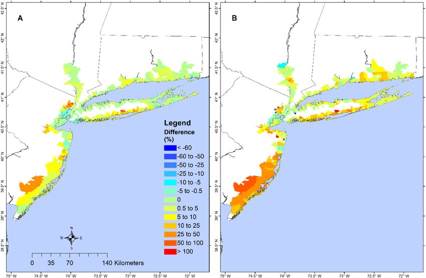
www.nature.com/scientificreports/
System (CH3D-SSMS), showed a significant reduction of total inundation volume by mangroves in Miami-Dade
County, Florida during Hurricane Andrew in 1992.
Recent studies showed contradictory findings on the value of coastal wetlands in reducing structure loss
along the New Jersey coast during Superstorm Sandy. Narayan et al.13 (hereafter referred to as NAR17), using a
2D hydrodynamic model and an industry-based flood and loss model to quantify the wetland value in terms of
structure losses, found that, on the zip-code level, wetlands helped to significantly avoid an average of 27% of
structure loss in NJ and up to 139% in south N J14. Paradoxically, their estimated avoided loss is only 3% over the
entire NJ, suggesting wetland had little impact. The percent avoided loss was calculated as the ratio of the avoided
loss (difference between the loss without wetland and the loss with wetland) divided by the loss with wetland. In
zip-code with low loss, however, the percent avoided loss became misleadingly high. Moreover, their assessed
loss was not verified with FEMA National Flood Insurance Program (NFIP) payout data, making it impossible
to validate their assessment. Their south NJ analysis was based on idealized (instead of actual) structure data
and the effect of wetland on reducing wave and wave-induced loss, which can be comparable to the flood loss,
was not explicitly addressed. Lathrop et al.15 (hereafter referred to as LAT19), on the other hand, used NFIP loss
payout data with actual structure and wetland data for south NJ constructed a regression model to relate the
structure losses to several factors and found that wetland had little effect on structure loss. Neither study was able
to convincingly relate the actual loss to the various contributing factors including wetland type and coverage,
wave and surge, and actual structural data. To resolve the conundrum created by these two studies, we present
a comprehensive study to elucidate the role of wetlands in affecting flood, wave, and structure loss during three
very different flood and wave events.
A typical “dynamics-based” assessment (as opposed to the “regression-based” assessment of LAT19) on the
value of wetland for flood reduction is done by simulating the flooding and wave caused by a hurricane, first
with and then without the w etland11–13,15–17. Loss associated with the flood and wave is then calculated with
and without the w etland13,16–18. However, there are large uncertainties associated with many aspects of this
“dynamics-based” assessment: accuracy of the simulated hurricane wind fields used for the surge-wave model,
model parameterization of surge-wave dynamics and vegetation processes, availability of wind-surge-wave data
during hurricanes for verification, accurate representation of the coastal wetland and properties, inclusion of
flood and wave losses, and parameterization of loss processes in the loss model, e tc19–21. Importantly, flood and
wave both contribute to structure loss, and wave-induced loss can exceed flood-induced loss for some storms.
Therefore, unless the assessment includes detailed verification of the simulated wind and surge-wave, as well as
estimated structure loss, the assessed loss reduction by wetland, could be highly uncertain and may be useless
for local resilience planning efforts.
The 2D approach using Manning coefficients to include the bottom friction and vegetation-induced friction
is the go-to methodology in most hurricane loss assessment studies, as in NAR17, although it has been shown
that the Manning coefficient is a function of vegetation structure and flow, thus making its parameterization very
complex and u ncertain22,23. Extensive water level and flow data are needed to tune the Manning coefficient which
is a function of space and time. Nevertheless, while the 3D model is preferred over the 2D model, we used the
2D version of CH3D-SSMS for this study due to lack of detailed coastal wetland structure data along the tristate
coasts. The simulated surge and wave during Sandy were verified with extensive field data, while the estimated
residential structure losses were verified with FEMA NFIP loss p ayouts24. Additionally, we assessed the role of
coastal wetlands in reducing loss during an extreme “Black Swan” storm (see “Methods” section for the rationale
behind the Black Swan storm) which made landfall near Staten Island, NY, and an ensemble of storms along the
tristate coasts. Real structure data, as opposed to idealized structural d ata13, were used in the loss analysis for
Sandy, the Black Swan storm, and ensemble of storms. Importantly, this study explicitly simulated the surge and
wave as dynamically coupled processes and calculated the loss by both flood and wave, while NAR17 simulated
the surge only and considered the wave effect “implicitly”13. While flood and wave analyses were done for the
tristate region, the loss analysis was done for NJ and parcel-specific loss analysis results were aggregated into
zip-code scale and state scale for in-depth analysis. Loss analysis for NY and CT could not be conducted due to
unavailability of structural data.
Results
Extensive hydrodynamic model validation. To provide a comprehensive validation of the modeled
surge-tide-wave dynamics during Sandy, this study made use of all available field data from an extensive network
of coastal water level gauges and wave buoys in the study region, as well as hundreds of HWMs and many rapid
deployment surge sensors (SI Fig. S1). The good agreements between simulated and observed water levels and
waves were quantified in terms of the root-mean-square error (RMSE) and correlation coefficient (CORR).
Storm tide. Available data included those from hundreds of permanent and temporary surge sensors from
NOAA (SI Fig. S2), Hudson River Environmental Conditions Observing System (HRECOS), and USGS. Sta-
tistics (SI Table S1) showed excellent agreement between the time series of simulated and measured storm tide
data. The averaged RMSE at USGS temporary sites was 0.20 m and the averaged CORR was 0.94. CH3D-SSMS
successfully reproduced the surge and tides with high confidence in not only the open ocean but also the com-
plex estuarine system during Sandy (SI Fig. S3) with a maximum coastal storm tide at NY Bight of 3.36 m and
NJ coast of 3.27 m.
High water marks and inundation. A total of 526 out of 653 independent HWM locations were located within
the study region, most of which clustered in NJ and NY coastal areas. 83.7% (440 out of 526) of HWMs were
captured by the CH3D-SSMS model grid and compared with the surveyed values. The model results had 0.33 m
Scientific Reports | (2021) 11:5237 | https://doi.org/10.1038/s41598-021-84701-z 2
Vol:.(1234567890)
www.nature.com/scientificreports/
RMSE and 0.87 CORR (SI Fig. S4). When only “good” and “excellent” HWMs (rated by USGS) were used, the
RMSE dropped to 0.30 m, and CORR increased to 0.90. The noticeable data disagreements (Fig. SI 4) were
caused by the inconsistency of surveyed data.
Wave. During Sandy, four wave-buoys within the domain recorded the wave data: two at the apex of NY Bight,
and another two in Long Island Sound (LIS). The significant wave height Hsig and peak wave period Tp simulated
by the Simulating Waves Nearshore (SWAN) model in the CH3D-SSMS were compared with measured data and
Wave Watch III (WW3) operational run results (SI Fig. S5)25,26. SWAN more accurately captured the evolution
of Hsig in NY Bight and LIS. Maximum significant wave height over land was as high as 2.17 m at NY Bight and
2.60 m along NJ coast.
Impact of wetland on surge and wave during super storm sandy. To estimate the value of the
coastal wetlands in reducing flood, we calculated the following four metrics for inundation: the Average Inunda-
tion Height ( AIH ), the Maximum Inundation Height ( MIH ), the Total Inundation Area (TIA), and the Total
Inundation Volume (TIV ) with and without wetlands. The TIA and TIV are defined as
TIA = dxdy, (1)
Landward area
(2)
TIV = [Hmax x, y − H0 x, y ]dxdy,
Landward area
where Hmax x, y and H0 x, y are the maximum water level and the land elevation at land cells x, y ,
respectively11,12. The wave analysis was carried out by calculating the average wave height ( AWH ), the maximum
wave height ( MWH ), and the total wave energy (TWE ) which is defined as
1
TWE = [ ρw g(Hrms max )2 ]dxdy, (3)
Landward area 8
where Hrmsmax is the maximum root-mean-square wave height over the flooded land. The wave energy, instead
of wave height, is more directly related to the wave-induced structure loss.
We define the relative inundation reduction ( RIR ) as the difference in TIV (value without wetland minus
value with wetland), divided by the TIV with wetland. The relative wave reduction ( RWR ) is defined accord-
ingly using the TWE . The inundation and wave analysis were carried out at the regional level (SI Table S2) and
zip-code resolution (Figs. 1, S6, S7).
If the wetlands were absent during Sandy, the RIR of the entire model domain would have been 4% and the
RWR would have been 19%. Breaking the entire model domain into 6 regions (Table S2): South NJ (SNJ), Central
NJ (CNJ), North NJ (NNJ), CT, Long Island (LI), and Mainland NY (MNY), it was found that the RIR during
sandy was low (< 10%) for all regions, while the RWR was moderate for CNJ and SNJ (10–25%) where the wet-
land cover was high, and low for the other regions. Although CT ranked 3rd in wetland cover, its RWR ranked
4th during Sandy due to Sandy’s landfall location and the sheltering of waves provided by LI which ranked 3rd.
Model simulations show that, during Sandy, if the wetland in the entire region were completely made up
of woody wetland, TIV and TWE would decrease by 9.1% and 12.4%, respectively, while increase by 1.2% and
2.2%, respectively, if the wetland were composed of marsh only. RIR and RWR for the all-marsh wetland are
6.5% and 19.1%, respectively, while those for the all-woody-wetland are 17.6% and 36.8%, respectively. These
results demonstrate that the woody wetland is much more effective than the marsh in buffering flood and wave.
Benefit of wetland on surge and wave during a Black Swan (BS) storm. We consider a rare “Black
Swan” (BS) storm (with a 0.0034 annual frequency vs. 0.0014 for S andy27) which made landfall in Staten Island
with a storm surge that surpassed the maximum surge during Sandy with maximum coastal values of 7.17 m at
NY Bight and 4.51 m at NJ coast of (Fig. S8). On the other hand, maximum significant wave heights over land
were not greater than those of Sandy: 1.99 m at the NY Bight and 2.12 m on the NJ coast, but average wave height
was higher than during Sandy (Fig. S8). During the Black Swan storm, wetlands created the biggest RIR and
RWR. MNY and NNJ experienced significant RIR, while the remaining regions experienced low RIR. In contrast
to Sandy, in which CT, MNY, and NNJ had less RWR, for the Black Swan storm these regions experienced high
(> 50%) RWR, while LI. CNJ and SNJ had significant (~ 25–50%) RWR. The regions with the highest RIR and
RWR were closest to the storm landfall location.
Benefit of wetland on surge and wave for the 1% annual chance flood. The maximum 1% annual
chance maximum flood elevation (Fig. S9) was 5.15 m for NY Bight while 5.34 m for the NJ coast. The 1% annual
chance maximum wave height (Fig. S9) overland is 2.24 m at NY Bight and 1.90 m at NJ coast. All the regions
had moderate RIR except for SNJ which had a significant RIR due to highest (25.4%) wetland cover (see Table S2)
and NNJ experienced significant RWR while the remaining regions had moderate values. CT ranked 2nd in RIR
although it has less wetland cover than CNJ because the mostly woody wetlands in CT are more effective in buff-
ering storm surge than the marshes in NJ and NY. On the other hand, CT ranked 3rd in RWR due to the blocking
of offshore wave energy by LI. RIR and RWR are found to be functions of storm characteristics, wetland type, and
cover, and local conditions. Fig. S10 shows the percent wetland cover, RIR (relative TIV reduction), and RWR
(relative wave energy reduction) in six regions (New York, North New Jersey, Long Island, Connecticut, Central
Scientific Reports | (2021) 11:5237 | https://doi.org/10.1038/s41598-021-84701-z 3
Vol.:(0123456789)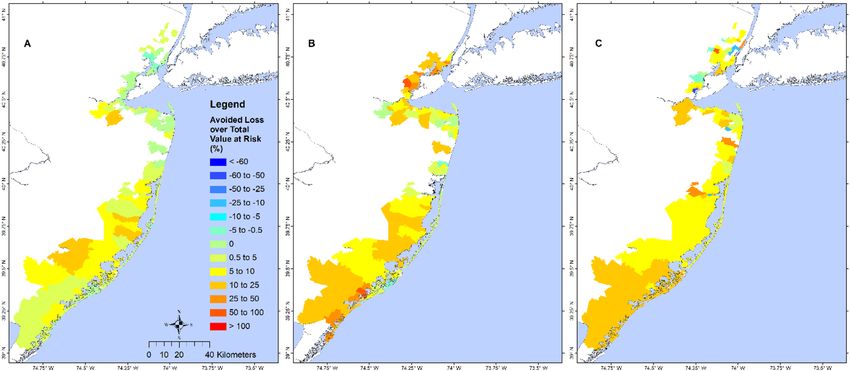
www.nature.com/scientificreports/
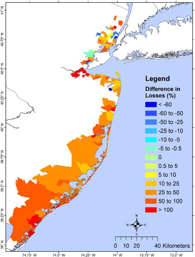
Figure 1. Zip-code resolution wetland’s effect on TIV and TWE during Sandy in 2012. Map showing zip-code
resolution avoidance in (A) TIV and (B) TWE during Sandy without wetlands, as a percentage of those for the
with-wetland scenario. Dark red values show zip-code with the most wetland benefit while dark blue areas have
the least wetland benefit. Negative values indicate that the presence of wetland would increase TIV /TWE and
positive values indicate that wetland would lower TIV /TWE . The map is produced using ESRI ArcGIS Pro 2.7
(https://www.esri.com/en-us/arcgis/products/arcgis-pro/overview).
New Jersey, and South New Jersey) during 1% annual chance events. As the wetland cover increases from less
than 5% (NY, NNJ, and LI) to more than 10% in CNJ and SNJ, RIR and RWR generally increase, showing the
increasing role of wetland in reducing inundation and wave. Relative reduction in inundation and wave energy
are modest, between 10 and 30%. NNJ has properties behind the relatively sparse marsh, followed by woody
wetland which protects properties behind them. Connecticut has less wetland than Central Jersey, but the mostly
woody wetland is more effective in reducing flood and wave.
Benefit of wetlands on reducing residential structure loss. The monetary loss of residential struc-
tures was estimated using the simulated inundation and wave results while employing damage functions from
the United States Army Corps of Engineer (USACE) North Atlantic Comprehensive Coastal Study (NACCS)
and was validated using the NFIP building loss payouts aggregated by zip-code21,24. Direct simulation of wave-
induced damage requires understanding and calculation of wave loads on structures using a depth- and phase-
resolving model, which is beyond the capability of the models used in this study. Therefore, in this paper, we
did not directly simulate wave-induced damage, but are accounting for wave-induced change in total water level
which results in increase in estimated damage based on depth-damage functions. Overall, 96 coastal zip-codes in
the state of NJ were used to validate the estimated loss. The model showed a correlation coefficient (CORR = 0.69)
between simulated structure losses and NFIP payouts (Fig. 2). In NJ, as of 2019, the total NFIP payout was $3.9
billion USD, in comparison to the estimated total structure loss of $3.6 billion USD (SI Table S3), with an abso-
lute error of 7.7%. This good agreement, plus the good agreement between the simulated and observed surge and
wave reported earlier, confirms the validity of our “dynamics-based” loss assessment.
We define the structural loss reduction (SLR ) as the structural loss without wetland minus the structural
loss with wetland, and the relative structural loss reduction ( RSLR ) as the ratio between SLR and the loss with
wetland. A state-level analysis of structure loss in NJ showed a RSLR of 8.5%, 26.0%, and 52.3% for Sandy, BS
storm, and 1% chance flood/wave, respectively (Table S3). Analysis of losses due to flood and wave indicated
that for Sandy and the 1% event, most of the loss came from flood, while most of the loss in the BS storm came
from waves. Avoided wave-induced loss was comparable to the avoided flood-induced loss during the BS storm
and the 1% event, but much higher during Sandy, suggesting that NJ wetlands are more effective in reducing
wave-induced loss vs. flood-induced loss. Results from the zip-code scale analysis during Sandy (Fig. 3) showed
Scientific Reports | (2021) 11:5237 | https://doi.org/10.1038/s41598-021-84701-z 4
Vol:.(1234567890)
www.nature.com/scientificreports/
Figure 2. Economic model validation at zip-code resolution. Simulated losses during Sandy in NJ using
the USACE damage functions versus FEMA NFIP payouts. Results were aggregated by zip-code and the
corresponding correlation coefficient is 0.69 (R2 = 0.47). Validation use transformed structure loss (PLT ) instead
of the structure loss (PL). The figure is produced using MATLAB R2020 (https://www.mathworks.com/).
less variability: for most north NJ, RSLR ranged from 10 to 100% except for those along the Hudson River that
had small increased loss (negative avoided loss). Most zip-codes in SNJ had RSLR between 5% and more than
100%. RSLR during the BS storm (Fig. S11) was more notable: ~ 50–100% for north NJ, 0–100% for central NJ.
The 1% flood event (Fig. 4) showed an average RSLR > 25% for NJ.
The above results showed that the value of coastal wetlands for flood/wave protection varies significantly with
the storm. While wetlands may be more effective in reducing wave loss in some storms but flood loss in other
storms, they may be ineffective in extreme storms. The 1% annual chance flood and wave event, which resulted
from an ensemble of many less extreme but more frequent s torms28, provides a more reasonable integrated
scenario for the loss analysis. This is similar to the preferred use of the 1% flood map, instead of the flood map
associated with a single design storm, for assessing the flood risk in any coastal region.
As shown in Fig. 5, in zip-codes with larger wetland coverage area in SNJ, wetlands could only pre-
vent < $25,000 annual loss (loss in the 1% event divided by 100), while wetlands in zip-codes with medium
wetland coverage area in central NJ could prevent > $60,000 annual loss. On the other hand, wetlands in north
NJ zip-codes with smaller wetland coverage area would increase the loss. The annual loss in most of the zip-codes
is < $10,000 except in one zip-code where the annual loss is ~ $50,000.
To explain the significant spatial variation in SLR by wetlands, we developed a generalized linear regression
model using the normal distribution with the logit link function, which was fitted with data for all coastal zip-
codes during three flood events and with and without wetlands. Percent wetland cover, percent at-risk structural
value, and average wave crest height in the zip-code were used as predictors to estimate the percent structural
loss (PSL = structural loss value divided by at-risk structural value) in the zip-code (Table 1). For Sandy, the
regression model had a significant correlation ( R2 = 0.75, p < 0.001). For the BS storm and the 1% annual chance
flood, there was a strong correlation with R2 = 0.87 and R2 = 0.84, respectively, both with p < 0.001. Using the
three storm scenarios, each with and without wetland, the regression fit (Fig. 6) had a significant correlation
with R2 = 0.75 and p < 0.001.
Discussion
In this paper, we presented the benefits of wetlands for reducing storm surge, waves, and structural losses during
Hurricane Sandy. Recent papers on this topic, such as NAR17 and LAT19, focused on the effects of wetlands on
reducing structure loss due to storm surge but did not include the effect of wetlands on reducing wave-induced
structural loss13,15. Estimated loss in NAR17 was not compared to NFIP payouts. LAT19 pointed out that veg-
etation has a dampening effect on wave energy, but waves were not included in their empirical NFIP pay-out
model due to lack of data15. NAR17 did not include the wave in their hydrodynamic model explicitly13, although
it is known that wave setup could contribute up to 20% of the peak s urge29 and wave can introduce additional
loss. Here, we showed how valuable these wetlands are in terms of reducing wave energy which could damage
structures and even cause deaths. Wetland effect on attenuating storm surge has been widely studied and the
attenuation effect increases with the wetland thickness, density, and height11. Our results showed that regions
with thicker, denser, and taller wetland cover reduced more TIV and TWE during Superstorm Sandy. Regions
Scientific Reports | (2021) 11:5237 | https://doi.org/10.1038/s41598-021-84701-z 5
Vol.:(0123456789)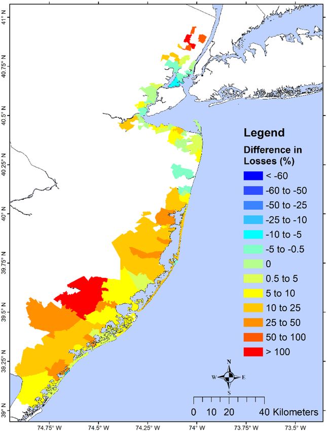
www.nature.com/scientificreports/
Figure 3. Percent structural loss reduction during Sandy. Map showing zip-code resolution avoided loss
(difference in loss without wetlands and loss with wetlands) during Sandy, as a percentage of the loss of the
with-wetland scenario. Dark red values show zip-code with the highest wetland benefit, while dark blue areas
have the least benefit. Negative values indicate that the presence of wetland would increase structural losses
and positive values indicate that wetland would lower the structural losses. The results are shown for the NJ
coastal zip-codes affected by Sandy. This study shows that the percent avoided loss in this figure does not always
represent the actual wetland value for loss reduction because areas with few structures and losses could give
misleadingly high values of percent avoided loss, as shown in south NJ. The primary purpose is for comparison
with a similar figure in NAR17. The map is produced using ESRI ArcGIS Pro 2.7 (https://www.esri.com/en-us/
arcgis/products/arcgis-pro/overview).
with highest wetland cover, hence more TIV and TWE reduction, were found in SNJ, CT, LI, CNJ, NNJ and
MNY, in descending order.
LAT19 observed that the extent of wetland on Barnegat-Great Bay did not have enough spatial extent and
height to dissipate the Superstorm Sandy s urge15. This is consistent with our finding that wetland dissipated
TIV by − 0.5% to 0.5%. Like NAR17, we found that landward zip-codes benefited from the surge attenuation at
coastal zip-codes13. Moreover, we found that wave attenuation at coastal zip-codes helped to reduce wave energy
at landward zip-codes. Our study showed notable TWE dissipation in SNJ where the landward zip-codes experi-
enced a cumulative reduction in surge and wave which translated into less structural loss (Fig. 3). For example,
in zip-code 08330 (Hamilton Township), wetland helped to avoid 41% of structural loss, far less than the 139%
AR1713. In contrast, we found that zip-code 08226 (Ocean City) had only a ~ 3% loss avoidance. The
reported in N
annual avoided losses for zip-code 08330 and 08226 were ~ $11,000 and ~ $3.6 million, respectively. This showed
that percent avoided loss is not a good index for characterizing the wetland value for protection against storm
surge and waves. Zip-code with low total structural value and low avoided loss, such as 08330, was estimated by
NAR17 to have a misleadingly high value of percent avoided losses.
Our estimated loss compared reasonably well with the NFIP loss payouts. The squared correlation coefficient
of 0.47 is much higher than the value of 0.184 of LAT19 who found no evidence that increasing marsh buffer
distance would reduce the amount of NFIP payouts for the nine south NJ t ownships15. LAT19’s suggestion that
NFIP payouts will increase by $4.05 per foot of marsh width was not supported by our dynamics-based economic
analysis15.
Our economic analysis slightly under-estimated the total NFIP payouts, probably because of some conserva-
tive assumptions. Our hydrodynamic model did not consider major rivers in NJ and did not include precipitation.
For simplicity, we used the 2D version of CH3D-SSMS with the Manning’s n coefficient representing the friction
by vegetation, land, and structures, which likely overestimated the friction effect and reduced the loss. During
Sandy, marsh stem height—usually lower than 30 cm in south NJ according to the 2012 land cover database of
Scientific Reports | (2021) 11:5237 | https://doi.org/10.1038/s41598-021-84701-z 6
Vol:.(1234567890)www.nature.com/scientificreports/
Figure 4. Effect of wetlands on structural losses over zip code scale during the 1% annual event. Map showing
zip code resolution difference in losses if the wetlands were absent, as a percentage of the wetland present
scenario. Dark red values show zip code with the highest benefit of having wetlands while dark blue areas show
the least benefited area. Negative values indicate that the presence of wetland would increase structural losses
and positive values indicate that wetland would lower the structural losses. The map is produced using ESRI
ArcGIS Pro 2.7 (https://www.esri.com/en-us/arcgis/products/arcgis-pro/overview).
the NJ Department of Environmental Protection (NJDEP)—was much lower than the storm surge, therefore
the actual marsh benefits were probably somewhat lower than that represented by the 2D m odel30. The effect of
wetland structure, as well as marsh distribution, on flood and wave dissipation, could be better represented by
using a 3D vegetation resolving model, e.g., Sheng et al.11, if detailed wetland data were available. Our structural
loss model did not include unavailable basement data which could have increased the losses. The Manning’s n
used in our simulation was 0.045 which is smaller than the value of 0.068 for rigid vegetation31 but very close
to the value of 0.049 for flexible vegetation when the empirical findings of Chapman et al.32 were used to adjust
the bulk drag coefficient in Luhar and Nepf31. If the Spartina-dominant marsh were replaced by a tall and
dense Phragmites-dominant marsh, Manning’s n would increase and result in less structural loss.
During the BS storm, NJ coast experienced a slightly higher surge but much higher wave, both significantly
buffered by the wetlands. Hence, the removal of wetlands would significantly increase the flood, wave, and loss
along the NJ coast than during Sandy. This showed that wetlands’ buffering capacity depends significantly on the
wetland structure/distribution, the characteristics of the hurricane, and the specific location of interest. To assess
the overall buffering capacity of tidal wetlands over a large region, an ensemble of storms should be considered
instead of 1–2 specific storms. To generate the 1% flood and wave event, 300+ “optimal storms” were generated
with the JPM-OS method and the CH3D-SWAN model based on the ensemble of storms generated by a statisti-
cal hurricane m odel26. Flood and wave associated with these optimal storms are being used to develop a Rapid
Forecast and Mapping System (RFMS)33 for NJ/NY/CT region, which can be used to predict real-time surge and
wave including wetland effects during any hypothetical storm.
The regression analysis shows that wetlands are more effective in reducing losses when the average wave
crest height is lower, which confirms that wetlands’ buffering capacity is more effective for low-intensity and
more frequent s torms16. Loss in a zip-code increased with the at-risk structural value and the average wave crest
height but decreased with percent wetland cover. Zip-codes with higher structural value benefited more from
wetland protection. Without any structure behind a wetland, the ecosystem service value of the wetland for flood
protection is zero. The regression model developed in this study can be used to estimate the impact of changing
wetland coverage on loss, e.g., doubling the wetland coverage in every NJ zip-code would decrease the average
loss in Sandy from 4 to 3%.
Although coastal wetlands were found to reduce structural loss during Sandy, their percent loss reduction
was found to be very modest (− 10% to + 50% for most except one zip-code) compared to 22–139%, reported
Scientific Reports | (2021) 11:5237 | https://doi.org/10.1038/s41598-021-84701-z 7
Vol.:(0123456789)www.nature.com/scientificreports/
Figure 5. Wetland annual avoided losses for all NJ zip-codes. Map showing zip-code resolution avoided losses.
Annual avoided loss is calculated as the difference in losses for the without wetland and with wetland scenarios
using the 1% annual chance flood and wave map and then dividing it by 100 years. Dark blue values show zip-
code with the lowest wetland value/benefit, while red areas have the highest wetland value/benefit. Negative
values indicate that the presence of wetlands would increase structural loss and positive values indicate that
wetlands would lower structural loss. Negative values are relatively small while only increasing losses by ~ $10
thousand per year. The map is produced using ESRI ArcGIS Pro 2.7 (https://www.esri.com/en-us/arcgis/produ
cts/arcgis-pro/overview).
Sandy Black Swan 1% annual chance All
Estimated coefficients
− 4.5960 − 4.5626 − 4.6232 − 5.3659
Intercept
(0.1663, 6.14E−68) (0.2007, 2.16E−54) (0.1330, 5.29E−90) (0.1295, 2.83E−176)
− 0.3750 − 0.4936 − 0.3759 − 0.5553
Wetland cover
(0.17477, 0.0332) (0.2440, 0.0446) (0.1627, 0.0218) (0.1487, 0.0002)
3.1588 4.7737 3.5424 4.0563
Total structure value at risk
(0.1526, 2.93E−50) (0.1813, 3.94E−63) (0.1206, 4.94E−77) (0.1182, 2.15E−142)
0.5809 0.5226 0.31778 0.83418
Average wave crest height
(0.0845, 9.02E−11) (0.0673, 6.27E−13) (0.0623, 7.46E−07) (0.0431, 7.58E−65)
N 191 181 218 590
R-squared 0.7487 0.8726 0.8359 0.7505
p-value 7.82E−56 6.36E−79 1.11E−83 3.52E−176
Table 1. Zip-code damage regression model estimates. The first value inside parenthesis represents the
standard error and the second value in parenthesis represents p-values.
by NAR17 in South NJ. At Himilton Township, NAR17 reported a dramatic 139% but LAT19 reported a slight
increase. The over-estimation of wetlands’ buffering capacity by NAR17 possibly resulted from the uncertain-
ties and lack of verification of their flood and loss analysis, not explicitly accounting for waves which contribute
significantly to loss, and the use of percent avoided loss as the sole indicator for wetland value. No attempt was
made to explain the effect of various contributing factors on the estimated losses.
Scientific Reports | (2021) 11:5237 | https://doi.org/10.1038/s41598-021-84701-z 8
Vol:.(1234567890)www.nature.com/scientificreports/
Figure 6. Zip-code structural loss regression model. A generalized regression model using a normal
distribution with a logit link function. Constructed using the Structure Value at Risk, Wetland Cover, and
Average Wave Crest Height as predictors to estimate structural losses in zip-codes ( R2 = 0.75, p < 0.001). Coupled
with a Rapid Forecast and Mapping S ystem33 being developed for the region, this regression model can be used
to forecast potential structural loss during an approaching hurricane. It can also be used to predict the potential
loss in any hypothetical hurricane, or to plan wetland restoration to reduce loss in any specific zip code. The
figure is produced using MATLAB R2020 (https://www.mathworks.com/).
Figure 7. Wetland value at zip-code level. Map showing zip-code resolution avoided losses during (A) Sandy,
(B) BS storm, and (C) 1% annual flood and wave, as a percentage of the total at-risk property value of the
without wetlands scenario. Dark red values show zip-code with the highest wetland value while dark blue areas
show the least wetland value. Negative values indicate that the presence of wetland would increase structural
losses and positive values indicate that wetland would lower the structural losses. These maps show that wetland
values for NJ are mostly between low (< 10%) and modest (10–25%). These maps, along with the wetland value
regression model developed in this study, can be used by local planners to develop resiliency and restoration
plans to increase the wetland coverage area and enhance the wetland value. Maps for NY and CT are unavailable
due to unavailability of structural data there. The map is produced using ESRI ArcGIS Pro 2.7 (https://www.esri.
com/en-us/arcgis/products/arcgis-pro/overview).
Scientific Reports | (2021) 11:5237 | https://doi.org/10.1038/s41598-021-84701-z 9
Vol.:(0123456789)www.nature.com/scientificreports/
This study showed that the percent structural loss (PSL) varies significantly across a coastal region depending
on percent wetland cover, at-risk structural value, and storm characteristics11 (represented by average wave crest
height). As shown in Fig. 7, the PSL for NJ is between low (< 10%) and moderate (< 25%). These maps, together
with the regression model can be used to develop wetland restoration plans (e.g., increasing wetland coverage
area) to reduce structural loss in the future. Adding the regression model to the RFMS will enable forecasting
of structural loss during a hurricane.
Strong winds during storms can directly damage coastal wetlands, resulting in reduced buffering capacity of
wetlands for coastal protection. Further studies are needed to fully understand the complex interactions among
wetlands (with different type, structure, density, and coverage area, etc.), storm surge and wave, erosion, wind,
and sea-level rise (SLR). With 1–2 m of SLR projected by 2100, tristate tidal marshes (with a height of 0.3–1 m)
can be easily overwhelmed and lose their buffering c apacity34. The approach presented in this study can be
expanded to develop and assess wetland restoration plans to mitigate future flood risk in the twenty-first century.
Methods
The role of coastal wetland in reducing coastal flood is analyzed by determining (a) the surge peak and extent, (b)
the significant wave height and peak wave energy, and (c) the resulting structural losses at all flooded locations
during three flooding events (Sandy, “Black Swan” storm, and the 1% annual chance flood and wave event). The
surge and significant wave height were estimated using a coupled surge-wave modeling system CH3D-SSMS
and the structural loss was estimated using the USACE depth damage f unctions19.
Hydrodynamic modeling. The coupled surge-wave model is based on CH3D-SSMS29,35,36. CH3D-SSMS
couples 2D/3D storm surge and wave models of coastal and basin scales using a non-orthogonal curvilinear grid
for the horizontal directions and a terrain-following sigma coordinate in the vertical direction for an accurate
representation of estuaries and coastal waters. In the coastal region, the surge model CH3D is dynamically cou-
pled to the wave model SWAN25,37,38. The governing modeling equations and surge-wave coupling mechanisms
of CH3D-SSMS were well documented in Sheng et al.29.
The study domain is represented by a high-resolution curvilinear grid which consist of 1461 by 2182 cells with
40–50 m resolution in NYC and about 20 m in the low-lying land area, such as lower-Manhattan, to resolve the
local complex geographic features. The grid domain covers the coasts of New Jersey, New York, and Connecti-
cut. It also includes the Hudson River from the New York Harbor to the Federal Dam at Troy. It extends from
the continental shelf to elevations that are higher than the possible extent of flooding by storm surge. The grid
in CT and NY reach elevations that are greater than 200 m and in NJ it is expanded 40+ km inland or reaching
elevations that are greater than 10 m. The model’s bathymetry and topography were generated using NOAA’s
National Centers for Environmental Information (NCEI) bathymetric and topographic telescoping digital eleva-
tion models (DEMs) of the U.S. Atlantic Coast impacted by Hurricane Sandy. This DEM resolution varies from
1/9 arc-sec (3.4 m) in the coastal zone to 3 arc-sec (90 m) in the offshore. For the locations where NCEI’s DEM
was not available, the 1/9 arc-sec DEMs from the U.S. Geological Survey (USGS) National Elevation Dataset
(NED) was used for land elevations, while NCEI’s Coastal Relief Model (CRM) was used for the water cells.
The Estuary Bathymetry data from the New York State Department of Environmental Conservation (NYSDEC)
was used in the Hudson River between Newburgh and Troy. These elevations were interpolated to the grid cells.
For this study, a 2D version of CH3D-SSMS was implemented with the use of Manning’s friction coefficient
(n) to account for the friction produced by vegetation and other land cover types. Higher values of Manning’s n
imply greater resistance to flow due to higher horizontal shear stress throughout the water column. Land Cover
types were obtained from the USGS 2011 National Land Cover Database (NLCD) which have a resolution of 30
m39. Manning’s n values were obtained from the land cover classes of the USGS NLCD based on the conversion
table from Mattocks and F orbes40. According to this, the coastal wetlands represented by emergent herbaceous
and woody wetlands have Manning’s n values of 0.045 and 0.1, respectively (Fig. S12).
Superstorm Sandy. The southern and eastern open ocean boundaries of the model are forced with linearly
added predicted tides and storm surge elevation. The tidal constituents used in the model are M2, N2, K1,
S2, O1, K2, and Q1 and they are obtained through the Advanced Circulation Model (ADCIRC) Tidal Dataset
(version ec2001)41. The surge boundary conditions for CH3D-SSMS were provided by an ADCIRC large-scale
model to incorporate the remote effects of storm surges9,10. Offshore wave conditions came from NOAA’s WW3
and river discharge data from the USGS. Two major rivers were included: the Hudson River at Green Island, NY
(USGS 01358000), and Connecticut River at Thompsonville, CT (USGS 01184000). Two high-resolution wind
fields, computed by the Regional Atmospheric Modeling System (RAMS), were applied as the meteorological
forcing. A wind field that covers a smaller spatial area with a spatial resolution of 6 km and a temporal resolution
of 15 min from Weatherflow, Inc. was merged with a larger spatial area wind field with a spatial resolution of
4 km and a temporal resolution of 1 h. These wind fields were also used by Wang et al.42 successfully to simulate
storm surge during Sandy.
A “Black Swan” storm. The Black Swan (BS) storm was designed as an extreme scenario of a Cat-3+ hurricane
such that winds of Category 1 hurricane intensity would be felt at the Village of Piermont, approximately 40 km
upstream of NYC along the Hudson River, after the landfall at Staten Island (Fig. S13). This storm would create
an extreme event in NJ because it moved northward very near the NJ shoreline. The wind field was generated
using the Holland wind model43 with a pressure deficit of 45 mbar, a radius to the maximum wind of 20 miles,
a forward speed of 5 mph, and a storm heading of -18 degrees from the north. Following Hall and S obel27,
this would create a storm with a 55° angle from perpendicular to the coastline with an annual frequency of
Scientific Reports | (2021) 11:5237 | https://doi.org/10.1038/s41598-021-84701-z 10
Vol:.(1234567890)www.nature.com/scientificreports/
0.0034 with a return period of 294 years. Along the NJ coast, extreme Black Swan winds would generate much
stronger surge and wave, and result in much higher structural loss and different wetland effects. At the Village
of Piermont, the peak wind speed during the Black Swan storm would be stronger than the peak wind speed
during Sandy, and the wind direction would be from the southeast instead of the east. This Black Swan wind
in the Piermont region was used in a separate study to investigate the role of the Piermont marsh in protecting
residential structures during storms.
Storm ensemble. Here, we consider a storm ensemble generated by Hall using the North Atlantic Stochastic
Hurricane Model (NASHM)44,45. Then, we used JPM-OS to generate a set of optimal storms to represent all the
possible storms described by Hall’s original storm ensemble28,46. Finally, we simulated the 1% annual chance
flood and significant wave height with and without the wetlands and produced the corresponding maps accord-
ing to the next equations:
P[ηmax > η] = ∫ · · · ∫ fx (x)P[η(x) > η]dx. (4)
Here, is the mean annual rate for all storms on the site, fx (x) is the joint probability density function of
the storm characteristics, and the conditional probability that a storm with certain characteristics x will cause a
water level height or significant wave height above η. This integral is evaluated for all possible combinations of
storm characteristics. The integral in Eq. (4) is not easily determined and is usually approximated as a weighted
summation of discrete storm parameters v alue28,46,47.
n
P[ηmax > η] = i P[η(xi ) > η]. (5)
i=1
Economic analysis. Following the procedure described in Loerzel et al.17, the economic analysis focused
on the state of NJ for simplicity. To quantify the value of the coastal wetland for flood and wave protection, two
simulations were performed, one with wetland and another without wetland. The without-wetland scenario
was done by replacing Manning’s n values of the wetlands with 0.02, which represents the open w ater13. For the
economic analysis, we identified the residential parcels that were flooded, as well as the inundation levels and
significant wave heights of each parcel. The structure value and the number of stories at every parcel are needed
to use the depth damage functions from USACE21.
The structural data used in this study included the residential parcels in the ‘Parcels and MOD-IV Composite
of New Jersey’ shapefile from the New Jersey Office of Information Technology, Office of GIS (NJOGIS)48. Base-
ments were unaccounted for due to lack of information. The value of the structure was assumed to be uniform
on any single parcel. Following Kousky and Walls49, a partially inundated parcel was included in the economic
analysis if and only if the parcel’s centroid is inside the inundation layer. The monetary value used in the analysis
for each parcel was the “improvement value” reported in 2018 USD. The loss percent was calculated using the
interpolated flood depth at each parcel centroid. Residential parcels without “improvement value” or building
description in terms of the number of stories were removed from the analysis. The numbers of stories were
rounded to the closest integer.
We combined flood and wave for economic analysis. First, the depth-limited controlling wave height is
calculated as Hc = min 0.78d, 1.6Hsig where d is the flood, and Hsig is the significant wave height. The next
step is to determine if the structure is in A zone, Coastal A zone, or V zone, according to FEMA. A zone is
defined as where Hc is lower than 1.5 ft, Coastal A zone is where waves are between 1.5 ft and 3.0 ft, and V
zone is where Hc is higher than 3.0 ft 50. Next, the total water depth above the first-floor elevation is calculated
as D = d + 0.7Hc − FFE for Coastal A and V zones and D = d − FFE for A zone, where FFE is the first-floor
elevation. Then we used this newly updated flood elevation which accounted for the wave crest for the USACE
NACCS damage functions. The wave damage functions were applied to structures in the V zone, and the flood
damage functions were applied to structures in Coastal A and A zones. The structural loss of each parcel ( PL) was
calculated by multiplying the structure damaged by the parcel “improvement value”. Finally, for validations pur-
pose only, we incorporated the maximum NFIP coverage for small structures by setting the transformed structure
loss PLT = min(PL, $250, 000). The total residential structural loss was then computed by adding together the
structural losses of each parcel ( PL) in the same zip-code. Avoided losses for every zip-code were calculated by
subtracting the structural losses of the wetland-absent case from that of the wetland-present case. We normal-
ized the NFIP payouts to 2018 USD using the county housing units51–53 and data reported in Weinkle et al.53.
It should be noted that the surge and wave were calculated by process-based dynamically coupled surge-
wave models and hence the simulated surge and wave contain nonlinear surge-wave interactions. On the other
hand, the damage assessment was based on empirical engineering understanding of flood and wave impact on
structures and used empirical formulations including empirically determined damage functions. In this study,
we followed the approach of USACE and FEMA without reinventing their empirical methods and formulas,
by using the 1% flood elevation and 1% wave height simulated by the coupled CH3D-SWAN model to better
represent the wave effect on total flood depth and damage. While this may not be the perfect approach for dam-
age assessment, our analysis provided a conservative damage estimation which probably slightly over-estimated
the total damage by using the sum of maximum flood and maximum wave as the total maximum flood depth
during each storm. Nevertheless, the good agreement between our assessed damage during Sandy and the NFIP
payouts confirmed the robustness of our method. Further improvement of the empirical damage assessment
may require additional data, model simulation, and parameter tuning which could be the topic of a future study.
Scientific Reports | (2021) 11:5237 | https://doi.org/10.1038/s41598-021-84701-z 11
Vol.:(0123456789)www.nature.com/scientificreports/
Data availability
The topography, bathymetry, and land-use datasets used in the regional and local studies are available via the
sources described above. The data on New Jersey structure value is available from https://njogis-newjersey.
opendata.arcgis.com/datasets/406cf6860390467d9f328ed19daa359d.The NFIP payout data is available from
https://www.fema.gov/media-librar y/assets/documents/180374. Damage functions are available from the U.S.
Army Corps of Engineers (Physical Depth Damage Function Summary Report, North Atlantic Comprehensive
Coastal Study: Resilient Adaptation to Increasing Risk). All derived data such as differences in losses and flood
and wave heights between the two scenarios for the regional study, are available from the corresponding author
on reasonable request and may be subject to a suitable Non-Disclosure Agreement.
Code availability
CH3D and SWAN have both been described in detail in the literature cited. Any inquiry about these models
should be directed to the corresponding author and TU-Delft, respectively. Wetland coverage data are available
from the corresponding author upon reasonable request.
Received: 3 November 2020; Accepted: 18 February 2021
References
1. Blake, E. S., Kimberlain, T. B., Berg, R. J., Cangialosi, J. P. & Beven, J. L. Tropical Cyclone Report Hurricane Sandy (AL182012) 22–29
October 2012. (2013).
2. Wikipedia. New York Metropolitan Area. https://en.wikipedia.org/wiki/New_York_metropolitan_area#cite_note-CombinedEs
t2016-14. Accessed 6 July 2017.
3. McCallum, B. E. et al. Monitoring storm tide and flooding from Hurricane Sandy along the Atlantic coast of the United States,
October 2012. Open-File Rep. https://doi.org/10.3133/OFR20131043 (2013).
4. Krauss, K. W. et al. Water level observations in mangrove swamps during two hurricanes in Florida. Wetlands 29, 142–149 (2009).
5. Shepard, C. C., Crain, C. M. & Beck, M. W. The protective role of coastal marshes: A systematic review and meta-analysis. PLoS
ONE 6, e27374 (2011).
6. Duarte, C. M., Losada, I. J., Hendriks, I. E., Mazarrasa, I. & Marbà, N. The role of coastal plant communities for climate change
mitigation and adaptation. Nat. Clim. Change 3, 961–968 (2013).
7. Möller, I. et al. Addendum: Wave attenuation over coastal salt marshes under storm surge conditions. Nat. Geosci. 7, 848–848
(2014).
8. Wamsley, T. V., Cialone, M. A., Smith, J. M., Atkinson, J. H. & Rosati, J. D. The potential of wetlands in reducing storm surge. Ocean
Eng. 37, 59–68 (2010).
9. Luettich, R. A., Westerink, J. J. & Scheffner, N. W. ADCIRC: An Advanced Three-Dimensional Circulation Model for Shelves Coasts
and Estuaries, Report 1: Theory and Methodology of ADCIRC-2DDI and ADCIRC-3DL, Dredging Research Program Technical Report
DRP-92–6. Dredging Research Program Technical Report DRP-92–6, U.S. Army Engineers Waterways Experiment Station, Vicksburg,
MS (1992).
10. Luettich, R. A. & Westerink, J. J. Formulation and Numerical Implementation of the 2D/3D ADCIRC Finite Element Model Version
44.XX (2004). https://adcirc.org/files/2018/11/adcirc_theory_2004_12_08.pdf. Accessed 15 July 2018.
11. Sheng, Y. P., Lapetina, A. & Ma, G. The reduction of storm surge by vegetation canopies: Three-dimensional simulations. Geophys.
Res. Lett. 39, 053577 (2012).
12. Sheng, Y. P. & Zou, R. Assessing the role of mangrove forest in reducing coastal inundation during major hurricanes. Hydrobiologia
803, 87–103 (2017).
13. Narayan, S. et al. The value of coastal wetlands for flood damage reduction in the northeastern USA. Sci. Rep. https://doi.
org/10.1038/s41598-017-09269-z (2017).
14. Danish Hydraulic Institute. MIKE 21 & MIKE 3 Flow Model FM Hydrodynamic Module: Short Description (2016).
15. Lathrop, R. G., Irving, W., Seneca, J. J., Trimble, J. & Sacatelli, R. M. The limited role salt marshes may have in buffering extreme
storm surge events: Case study on the New Jersey shore. Ocean Coast. Manage 178, 104803 (2019).
16. Rezaie, A. M., Loerzel, J. & Ferreira, C. M. Valuing natural habitats for enhancing coastal resilience: Wetlands reduce property
damage from storm surge and sea level rise. PLoS ONE 15, e0226275 (2020).
17. Loerzel, J. et al. Economic valuation of shoreline protection within the Jacques Cousteau National Estuarine Research Reserve (2017)
https://doi.org/10.7289/V5/TM-NOS-NCCOS-234.
18. Narayan, S. et al. Valuing the Flood Risk Reduction Benefits of Florida’s Mangroves (The Nature Conservancy, 2019). Accessed 10
October 2019.
19. U.S. Army Corps of Engineers (USACE). Economic Guidance Memorandum (EGM) 04–01, Generic Depth-Damage Relationships
for Residential Structures with Basements. (2003). https://planning.erdc.dren.mil/toolbox/librar y/EGMs/egm04-01.pdf. Accessed
10 October 2019.
20. Federal Emergency Management (FEMA). Multi-hazard Loss Estimation Methodology. Flood Model. HAZUS\Textregistered-MH
MR5. Technical Manual (2006). https://www.fema.gov/media-librar y-data/20130726-1820-25045-8292/hzmh2_1_fl_tm.pdf.
Accessed 3 August 2019.
21. U.S. Army Corps of Engineers (USACE). Physical Depth Damage Function Summary Report, North Atlantic Comprehensive Coastal
Study: Resilient Adaptation to Increasing Risk (2015). http://www.nad.usace.army.mil/Portals/40/docs/NACCS/10A_PhysicalDe
pthDmgFxSummary_26Jan2015.pdf. Accessed 4 November 2017.
22. Lapetina, A. & Sheng, Y. P. Three-dimensional modeling of storm surge and inundation including the effects of coastal vegetation.
Estuaries Coasts 37, 1028–1040 (2014).
23. Lapetina, A. & Sheng, Y. P. Simulating complex storm surge dynamics: Three-dimensionality, vegetation effect, and onshore sedi-
ment transport. J. Geophys. Res. Ocean. 120, 7363–7380 (2015).
24. National Flood Insurance Program (NFIP). FEMA NFIP Redacted Claims Data Set (2019). https://www.fema.gov/media-librar y/
assets/documents/180374. Accessed 1 December 2019.
25. Booij, N., Ris, R. C. & Holthuijsen, L. H. A third-generation wave model for coastal regions: 1. Model description and validation.
J. Geophys. Res. Ocean. 104, 7649–7666 (1999).
26. The WAVEWATCH III Development Group (WW3DG). User manual and system documentation of WAVEWATCH III version
6.07 Tech. Note 333, NOAA/NWS/NCEP/MMAB (2019).
27. Hall, T. M. & Sobel, A. H. On the impact angle of Hurricane Sandy’s New Jersey landfall. Geophys. Res. Lett. 40, 2312–2315 (2013).
28. Yang, K., Paramygin, V. A. & Sheng, Y. P. An objective and efficient method for estimating probabilistic coastal inundation hazards.
Nat. Hazards 99, 1105–1130 (2019).
Scientific Reports | (2021) 11:5237 | https://doi.org/10.1038/s41598-021-84701-z 12
Vol:.(1234567890)www.nature.com/scientificreports/
29. Sheng, Y. P., Alymov, V. & Paramygin, V. A. Simulation of storm surge, wave, currents, and inundation in the outer banks and
Chesapeake bay during Hurricane Isabel in 2003: The importance of waves. J. Geophys. Res. Ocean. 115, C04008 (2010).
30. New Jersey Department of Enviromental Propetction (NJDEP). New Jersey Land Use/Land Cover (LU/LC) (2015). https://www.
state.nj.us/dep/gis/lulc12.html.
31. Luhar, M. & Nepf, H. M. From the blade scale to the reach scale: A characterization of aquatic vegetative drag. Adv. Water Resour.
51, 305–316 (2013).
32. Chapman, J. A., Wilson, B. N. & Gulliver, J. S. Drag force parameters of rigid and flexible vegetal elements. Water Resour. Res. 51,
3292–3302 (2015).
33. Yang, K., Paramygin, V. A. & Sheng, Y. P. A rapid forecasting and mapping system of storm surge and coastal flooding. Weather
Forecast. 35, 1663–1681 (2020).
34. Sweet, W. V. et al. Global and Regional Sea Level Rise Scenarios for the United States (2017). https: //tidesa ndcur rents .noaa.gov/publi
cations/techrpt83_Global_and_Regional_SLR_Scenarios_for_the_US_final.pdf. Accessed 8 December 2017.
35. Sheng, Y. P., Zhang, Y. & Paramygin, V. A. Simulation of storm surge, wave, and coastal inundation in the Northeastern Gulf of
Mexico region during Hurricane Ivan in 2004. Ocean Model. 35, 314–331 (2010).
36. Paramygin, V. A., Sheng, Y. P. & Davis, J. Towards the development of an operational forecast system for the Florida coast. J. Mar.
Sci. Eng. 5, 8 (2017).
37. Sheng, Y. P. A Three-Dimensional Mathematical Model of Coastal, Estuarine and Lake Currents Using Boundary-fitted Grid. Techni-
cal Report No. 585 (1986).
38. Sheng, Y. P. Evolution of a three-dimensional curvilinear-grid hydrodynamic model for estuaries, lakes and coastal waters: CH3D.
In Estuarine and Coastal Modeling, 40–49 (1989).
39. Homer, C. G. et al. Completion of the 2011 National Land Cover Database for the conterminous United States—Representing a
decade of land cover change information. Photogramm. Eng. Remote Sensing 81, 345–354 (2015).
40. Mattocks, C. & Forbes, C. A real-time, event-triggered storm surge forecasting system for the state of North Carolina. Ocean Model.
25, 95–119 (2008).
41. Mukai, A. Y., Westerink, J. J., Luettich, R. A. J. & Mark, D. Eastcoast 2001, A Tidal Constituent Database for Western North Atlantic,
Gulf of Mexico, and Caribbean Sea (2002).
42. Wang, H., Loftis, J., Liu, Z., Forrest, D. & Zhang, J. The Storm Surge and Sub-Grid Inundation Modeling in New York City during
Hurricane Sandy. J. Mar. Sci. Eng. 2, 226–246 (2014).
43. Holland, G. J. An analytic model of the wind and pressure profiles in hurricanes. Mon. Weather Rev. 108, 1212–1218 (1980).
44. Hall, T. M. & Jewson, S. Statistical modelling of North Atlantic tropical cyclone tracks. Tellus Ser. A Dyn. Meteorol. Oceanogr. 59,
486–498 (2007).
45. Hall, T. & Yonekura, E. North American tropical cyclone landfall and SST: A statistical model study. J. Clim. 26, 8422–8439 (2013).
46. Condon, A. J. & Sheng, Y. P. Optimal storm generation for evaluation of the storm surge inundation threat. Ocean Eng. 43, 13–22
(2012).
47. Niedoroda, A. W. et al. Analysis of the coastal Mississippi storm surge hazard. Ocean Eng. 37, 82–90 (2010).
48. NJ Office of Information Technology-Office of GIS (NJOGIS). Parcels and MOD-IV Composite of New Jersey (2019). https://njogi
s-newjersey.opendata.arcgis.com/datasets/406cf6860390467d9f328ed19daa359d. Accessed 15 January 2020.
49. Kousky, C. & Walls, M. Floodplain conservation as a flood mitigation strategy: Examining costs and benefits. Ecol. Econ. 104,
119–128 (2014).
50. Federal Emergency Management (FEMA). Coastal Mapping Basics | FEMA Region II. http://www.region2coastal.com/resources/
coastal-mapping-basics/. Accessed 16 January 2020.
51. Collins, D. J. & Lowe, S. P. A Macro Validation Dataset for U.S. Hurricane Models. Casualty Actuarial Society Forum (Casualty
Actuarial Society, Arlington, 2001).
52. Pielke, R. A. et al. Normalized hurricane damage in the United States: 1900–2005. Nat. Hazards Rev. 9, 29–42 (2008).
53. Weinkle, J. et al. Normalized hurricane damage in the continental United States 1900–2017. Nat. Sustain. 1, 808–813 (2018).
Acknowledgements
This work was sponsored by the National Estuarine Research Reserve System Science Collaborative, which sup-
ports collaborative research that addresses coastal management problems important to the reserves. The Science
Collaborative is funded by the National Oceanic and Atmospheric Administration and managed by the University
of Michigan Water Center (NAI4NOS4190145). We also appreciate the support from the NOAA Climate Program
Office Grant NA11OAR4310105. We thank Harry Wang for providing the wind field data for Sandy simulation,
Timothy Hall for providing the storm ensemble data from NASHM model prediction, and Richard Lathrop for
providing marsh data in the Jacques Cousteau National Estuarine Research Reserve in South New Jersey.
Author contributions
Y.P.S. designed the study, supervised the model simulations and analysis, and wrote the main manuscript text.
A.R.N. and R.Z. conducted the model simulations of laboratory and field data. A.R.N. and V.A.P. conducted
the economic analysis and contributed to the writing of the manuscript text. R.Z. conducted the original Sandy
simulation in the large and small domains. A.R.N. developed the regression model. V.A.P. simulated the 1%
flood and wave event.
Competing interests
The authors declare no competing interests.
Additional information
Supplementary Information The online version contains supplementary material available at https://doi.
org/10.1038/s41598-021-84701-z.
Correspondence and requests for materials should be addressed to Y.P.S.
Reprints and permissions information is available at www.nature.com/reprints.
Publisher’s note Springer Nature remains neutral with regard to jurisdictional claims in published maps and
institutional affiliations.
Scientific Reports | (2021) 11:5237 | https://doi.org/10.1038/s41598-021-84701-z 13
Vol.:(0123456789)You can also read