Environmentally Extended Input-Output Analysis - SOCIAL ECOLOGY WORKING PAPER 154 - BOKU
←
→
Page content transcription
If your browser does not render page correctly, please read the page content below
S O C I A L       E C O L O G Y     W O R K I N G     P A P E R     1 5 4

                                    Anke Schaffartzik • Magdalena Sachs •
                                  Dominik Wiedenhofer • Nina Eisenmenger

   Environmentally Extended Input-Output Analysis

 ISSN 1726-3816                                             September 2014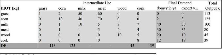
Anke Schaffartzik, Magdalena Sachs, Dominik Wiedenhofer,
Nina Eisenmenger (2014):

Environmentally Extended Input-Output Analysis

Social Ecology Working Paper 154
Vienna, September 2014

ISSN 1726-3816

Institute of Social Ecology
IFF - Faculty for Interdisciplinary Studies (Klagenfurt, Graz, Vienna)
Alpen-Adria-Universitaet
Schottenfeldgasse 29
A-1070 Vienna

www.aau.at/socec
workingpaper@aau.at

© 2014 by IFF – Social Ecology

Environmentally Extended Input-Output
                    Analysis

Authors:
Anke Schaffartzik
Magdalena Sachs
Dominik Wiedenhofer
Nina Eisenmenger
Table of Contents 1. Introduction ............................................................................................................................ 1 2. The Basics of Input-Output Analysis ..................................................................................... 2 2.1 Introduction to Input-Output Tables.............................................................................................. 2 2.2 Input-Output Analysis and the Leontief Inverse ........................................................................... 4 3. Environmentally Extended Input-Output Analysis (EEIOA) ................................................ 8 3.1 Leontief’s Example ....................................................................................................................... 8 3.2 EEIOA Example for a Hypothetical Economy ........................................................................... 11 4. Call for Caution .................................................................................................................... 14 5. References ............................................................................................................................ 17 Figures and Tables Table 1: Simplified Input-Output Table for a Hypothetical Three-Product............................... 3 Table 2: Overview of Typical Element Notation within an Input-Output Table ....................... 3 Table 3: Matrix A of Technical Coefficients for a Hypothetical Three-Product Economy ....... 6 Info-Box: Power Series Approximation..................................................................................... 7 Table 4: Leontief Inverse for a Hypothetical Three-Product Economy ..................................... 8 Figure 1: Environmental extension of the IO framework based on the physical input-output table (PIOT) as originally presented by Leontief ..................................................................... 10 Figure 2: PIOT, MIOT, and Leontief inverses for six-activity hypothetical economy............ 12 Figure 3: Material requirements associated with domestic and exported final demand (yd and yex) in the hypothetical economy ............................................................................................ 13
1. Introduction
Social ecology research centers on the understanding that in order to contribute to meaningful
analysis of current sustainability challenges, it is necessary to consider both sociocultural and
biophysical interrelations (Fischer-Kowalski and Weisz, 1999). It may seem self-evident that
economies indispensably require energy and material inputs as well as the discharge of wastes
in order to function. Yet, a dominant paradigm maintains that boundless economic growth is
possible. Such an approach to development does not take into account the biophysical
limitations of society’s metabolism and thus ignores given “limits to growth” (Ayres and
Kneese, 1969; Daly, 1973; Meadows et al., 1972). Nonetheless, important advances have been
made in considering human societies not only in terms of their economic but also their
biophysical dimensions in acknowledging that societies do have a “metabolism” (Fischer-
Kowalski and Haberl, 1998). Alongside the concept of social metabolism, a corresponding tool
was developed which, instead of regarding an economy purely in monetary terms, accounts for
society’s biophysical inputs and outputs. Economy-wide material flow accounts document
material use in mass units, most commonly metric tons. The considered material flows include
all materials an economy extracts from its domestic environment, imports from other and
exports to other economies as well as discharges to the environment (Fischer Kowalski et al.,
2011; Weisz et al., 2007). From its beginnings in academia, this approach continuously gained
wider acceptance together with the notion that growth in a physically finite world must be
limited. Indicators derived from material flow accounts have become an integral part of
environmental accounting (European Commission, 2011).
As the underlying methodology matured, so did the interest in applying it to new research
questions. As we potentially face planetary boundaries (Rockström et al., 2009), these
increasingly relate to understanding what drives (and has the potential to curb) our global
resource use. The latter requires a more in-depth understanding of the structures and dynamics
of resource use than can be gained from material flow accounts. The ‘black box’ as which MFA
treats society must be opened. In this Working Paper, we will examine the application of
economic input-output modelling in social ecology as a means to open up this black box. Input-
output models are used in economics to represent the structure of production and final
consumption within an economy (single-region input-output SRIO model) or amongst multiple
economies (multi-region input-output MRIO model). These models depict by economic activity
(e.g. agriculture, food production, restaurant services) the inputs required from other economic
activities (e.g. food production would buy inputs from agriculture and restaurant services would
buy inputs from food production) and the output provided either to other activities or to final
consumption (including public as well as private spending as well as exports). Although this
type of structure could also be depicted in physical units of mass or energy, data is typically
only collected in monetary units (see Weisz and Duchin, 2006) and serves as the basis for
calculating the gross domestic product (GDP) as the market value of all goods and services
produced within an economy during a specific year. Input-output data can be used to trace the
impact of changes in final consumption on production structures. Such an application also
allows for the calculation of the inputs required to produce goods and services for export.
Input-output analysis can be “environmentally extended” (environmentally extended input-
output analysis (EEIOA)) by integrating information from physical accounting, for example,
on energy or material use or pollution, into the input-output model. Because the input-output
model is in monetary units and the environmental extension is in physical units (e.g. in joules
of energy, tons of material, or kilograms of pollutant), this integration is non-trivial. A number
of assumptions have to be made, the validity of which has a significant impact on how we can

                                                1
interpret the results (see section 4). EEIOA is increasingly being used as a tool to understand
the material or energy requirements or the environmental burden associated with specific
sectors or with the components of final demand, e.g., for domestic final demand and exports.
Where the input-output table is extended by material flows, material inputs are allocated to
production sectors and can then be linked to the final demand which they ultimately satisfy.
With regard to exports, EEIOA allows for an approximation of the upstream material
requirements of the production of traded goods. Resource extraction, not matter where in the
world it occurs, is linked to the final demand for goods and services in the country under
investigation. This type of consumption-based approach to material flow accounting
complements the production-based approach (oriented towards the material use in national
economies).
In order to be able to interpret these types of accounts, it is important that the social ecologist
have a working knowledge of the fundamentals of environmentally extended input-output
analysis and be familiar with applications and limitations of the method. In this Working Paper,
we will provide an introduction to input-output analysis and its environmental extension
including step-by-step calculations based on the model of a hypothetical economy. We follow
up with a discussion of the assumptions which go into this type of approach. The aim of this
Working Paper is to make the important EEIOA tool accessible to students and researchers of
social ecology.
2. The Basics of Input-Output Analysis
In the following section, we will provide a very basic introduction to the general structure of
and calculations behind environmentally extended input-output analysis. Readers wishing to
study the method in greater detail and variation will find a wealth of useful information in the
standard textbook by Miller and Blair (2009) and the manual provided by Eurostat (2008). We
will begin with an introduction to the structure and elements of input-output tables and then
move on to the logic and the calculations behind their environmental extension.
2.1 Introduction to Input-Output Tables
Input-output tables (IOTs) depict the structure of an economy and include both the inter-
industry relations in its productive and service sectors and the composition of final demand.
The inputs required by each economic activity (or sector) to produce that activity’s output to
both other activities and to final demand are recorded. Although it is possible to construct IOTs
in physical units (tons, for example), sufficiently robust data for such tables is hardly available
in practice (see Weisz and Duchin, 2006). In monetary units, IOTs are compiled routinely by
the national statistical offices1 and, since they record the value of all goods and services
produced for final consumption in an economy within a given year, serve as the basis for
calculating the gross domestic product (GDP).
1
For example, the Austrian supply, use, and input-output tables are available here:
http://www.statistik.at/web_en/statistics/national_accounts/input_output_statistics/index.html. Eurostat publishes
the input-output tables of all EU member states here:
http://epp.eurostat.ec.europa.eu/portal/page/portal/esa95_supply_use_input_tables/data/workbooks.
2Table 1: Simplified Input-Output Table for a Hypothetical Three-Product
Wood Paper Books Final Demand Total Output
Wood 85 90 0 20 195
Paper 10 10 90 200 310
Books 5 5 20 500 530
Value Added 95 205 420 720
Total 195 310 530 720 1755
Table 1 depicts a simplified IOT of a hypothetical economy which only produces three goods
(and these goods are produced by three corresponding economic activities): wood, paper, and
books. The values in the columns show which inputs are required for the production of all the
wood, paper, and books in this economy. For example, 90 units worth of wood, 10 of paper,
and 5 of books are needed to produce the total amount of paper. While the top left 3x3 section
of the table depicts the inter-industry flows, the fourth column shows the final demand. Final
demand is shown as an aggregate value in this example. In ‘real-life’ input-output tables,
domestic and foreign final demand (exports) are typically differentiated. Domestic final
demand usually consists of the final demand of households and government and NGOs.
Changes in inventories and capital formation (gross fixed capital formation GFCF) are also
commonly reported as categories of final demand. For the latter category the argument might
be made that capital formation corresponds to inputs into (future) production. The total output
of each of the products corresponds to the sum of inter-industry use and final demand and is
represented in the column on the very right. In monetary terms, value is added to a product
during the production process. This happens because labor, taxes, interest, rent, and profit have
to be paid for. The value added is shown in the fourth row. Only as many units of a product can
be consumed within the economy as are generated. Therefore, the totals by column and by row
have to match.
Table 2: Overview of Typical Element Notation within an Input-Output Table
1 2 … j y x matrix Z with elements zij: interindustry flows
1 z11 z12 … z1j y1 x1
vector y with elements yi: final demand
2 z21 z22 … z2j y2 x2
… … … … … … … vector x with elements xi: total output
i zi1 zi2 … zij yi xi
v vector v with elements vi: value added
v1 v2 … vi
x' x1 x2 … xi Y X vector x’ with elements xi: total outlays
In order to facilitate our communication about input-output tables, we can use typical matrix
notation. The input-output table can be divided into several sections or matrices and vectors:
The interindustry relations, i.e. the 3x3 matrix with wood, paper, and books heading the
columns and the rows in Table 1, is often denoted by the capital letter Z. Its elements can
accordingly be represented by z11, z12, …, zij where the first index (i) represents the row number
and the second index (j) represents the column number corresponding to the element (see Table
32). In Table 1, for example, the flow of books into paper production would be represented by
element z32. The input-output table also contains a vector y of final demand (represented by a
single vector in Table 1 and 2 but often disaggregated by household and government
consumption as well as exports in ‘real’ IOTs). Vector x contains the total output (whether for
interindustry use or final demand) by each economic activity. Transposed into a row vector (x’),
it is usually referred to as total outlays. The elements in both vectors are identical because total
outlays must equal total output for each activity or product. The vector v represents the value
added.
Within the input-output table, total inputs equal total outputs: This is the mass balance principle
in economic terms. In simplified terms, the economic value of the all the flows into one activity
equal the value of all of the flows from that activity to other activities or final demand, for
example:
z11 + z12 + … + z1j + y1 = z11 + z21 + … +zi1 +v1 = x1 (Table 2)
and
85 + 90 + 0 + 20 = 85 + 10 + 5 + 95 = 195 (Table 1)
For the sake of simplicity, all of the following calculations refer to square (n x n) matrices, i.e.
to matrices with the same number of rows and columns (n). Input-output tables may, however,
be asymmetrical (i.e., non-square) and depict more than one type of output from each industry,
for example.
2.2 Input-Output Analysis and the Leontief Inverse
The term “input-output analysis” is often used to indicate that input-output structures are being
investigated on the basis of input-output tables. We will deal here with only one very central
aspect of this analysis which will be decisive for our environmental extensions: The Leontief
inverse. This calculation is named in honor of the Russian economist Wassily Leontief who
laid the methodological groundwork on which present-day EEIOA is based (Leontief, 1970,
1986).
Before we delve into the calculations: Why do we even need to calculate anything further? The
input-output table for our hypothetical economy (Table 1) informs us on how much wood,
paper, and books were needed to produce the 20 units worth of wood, 200 units of paper, and
500 units of books required by final demand. Often, however, we will be interested in
understanding the intermediate inputs associated with one unit of final demand rather than with
the total final demand. We might ask questions like: How much wood must be bought in order
to produce one unit of books for final demand? How much wood could be ‘saved’ if we reduced
final demand by one unit? If final demand for books increases by one unit, what would be the
effect on the wood and paper producing activities? We cannot answer these questions directly
based on Table 1 but a few simple mathematical equivalence operations will get us there.
The first transformation we will perform yields the matrix of direct intermediate input
requirements (also called technical coefficients) which is denoted by the capital letter A. Each
element in aij in A will represent the amount of inter-industry inputs directly required to produce
one unit of output. The calculation in itself is very simply: Each element of the matrix of
interindustry flows Z is divided by the total output (x) of that activity to which it contributes.
In matrix notation this calculation reads:
4= × (F1)
In order to divide each element of Z by the corresponding total output, we multiply Z with
diagonalized (indicated by the hat symbol) inverse (indicated by -1) of x. Multiplying with the
inverse is equivalent to dividing and the diagonalization (into an nxn matrix with the values of
x-1 along the diagonal) allows us to use matrix multiplication. For our example (Table 1) both
the inverse of x (x-1) and the diagonalization of that inverse ( ) are shown below:
0.005 (F2)
= 0.003
0.002
0.005 0 0 (F3)
= 0 0.003 0
0 0 0.002
By multiplying the matrix Z of interindustry flows (from Table 1) with the diagonalized inverse
of total production (F3), we obtain the matrix of technical coefficients A:
85 90 0 0.005 0 0 . . (F4)
= 10 10 90 × 0 0.003 0 = . . .
5 5 20 0 0 0.002 . . .
Please note that the vector in F2 and the matrix F3 have been rounded to the third decimal place.
Therefore, the calculation in F4 will render a slightly different result if the rounded values are
copied; the result presented in F4 stems from matrix multiplication using spreadsheet software
and is not based on rounded values. The value “0” (with no decimal places reported) represents
a true (and not a rounded) zero. Since all we have done is transform matrix Z, we can also easily
‘reverse’ our calculations: If we have calculated A correctly, then multiplying it with the
diagonalized vector of total output ( ) will yield matrix Z.
This matrix A of technical coefficients allows us to easily assess the amount of inter-industry
inputs required to produce one unit’s worth of output to final demand. For example, in order to
supply one unit of paper to final demand, 0.29 units of wood were directly required (element
a12 in Table 3). Please note that in spreadsheet software the symbol “-” (a13 in Table 3) is
sometimes used to represent a ‘true’ (as opposed to a rounded) zero. If the value in a13 in this
case were “0.00”, this would mean that the cell contains a value larger than zero rounded to the
nearest hundredth.
5Table 3: Matrix A of Technical Coefficients for a Hypothetical Three-Product Economy
Wood Paper Books
Wood 0.44 0.29 -
Paper 0.05 0.03 0.17
Books 0.03 0.02 0.04
Rather than assessing only the direct inputs required to produce a specific amount of output, we
may be much more interested in finding out something about the indirect input requirements as
well. For example, if, in order to provide one additional unit of books for final consumption,
matrix A indicates that no wood was required. But we may assume that wood had to be
purchased to make the paper to make the books. 0.02 units of books were directly required
(element a32 in Table 3) to produce one unit of paper: We may wish to find out how much paper
would be required to produce those books. Then, if the paper industry has to provide more units
of paper to produce the 0.02 additional units of books, it will also require other additional inputs
of wood and books. The wood and book industries in turn will then need additional inputs to
produce for the higher demand in the paper industry and so and so forth. If we wanted to
calculate the indirect requirements associated with any change in final consumption, we would
essentially need to reiterate the same calculation procedure over and over again until we arrived
at a result that was satisfactorily fitting. The fact that Leontief developed a calculation (centered
on the so-called Leontief inverse) which can be used instead of this approximation via re-
iteration makes our lives much easier.
In order to derive the so-called Leontief inverse which will allow us to account for both direct
and indirect inputs, we will first briefly return to our matrix A (F4).If we multiply A with the
vector of total output x, we obtain a vector the elements of which correspond to the difference
between total output x and final demand y, i.e. to total inter-industry flows such that:
× = - (F5)
Based on this equation, we can perform a series of equivalence operations to arrive at the
Leontief inverse:
= - (F5.1)
= ( - ) (F5.2)
=( - ) × (F6)
Note that the capital letter I denotes to so-called identity matrix which is matrix notation for 1
and consists of a matrix with ones along the diagonal and zeroes in all other places. The
following example is a 3x3 identity matrix as we would need it for all calculations for our
hypothetical economy (Table 1):
1 0 0 (F7)
= 0 1 0
0 0 1
6The elements in the Leontief inverse ( - ) reflect both the inputs required directly and
indirectly to produce one (additional) unit of final demand. The matrix in parentheses is taken
to the power of negative 1: This is the inverse of the matrix. The inverse of a matrix C is defined
such that × = where I is the identify matrix (see F7). Not all matrices are invertible: A
matrix for which the determinant (det(C)) is equal to 0 is a singular, non-invertible matrix. The
determinant of a matrix
=
is calculated as det( ) = ( + + )-( + +
).
Info-Box: Power Series Approximation
How the simple-looking equation ( - ) can reflect both the inputs required directly and indirectly to
produce one (additional) unit of final becomes clearer when we consider how we would calculate the
approximation of direct and indirect inputs in a re-iterative procedure. Such a procedure exists because the
inversion of large matrices requires quite some computational power which was not always available: Miller
and Blair (2009) report that in 1939, it took 52 hours to invert a 42x42 matrix and even in 1970, Leontief warned
his readers that computing the inverse for larger matrices would require a computer, indicating that he did not
use one for the examples with which he illustrated his approach (Leontief, 1970). The procedure by which the
Leontief inverse can be approximated without requiring the calculation of an actual inverse is known as the
power series approximation.
If we take a power series L such that
= + + + + + (F8)
and we multiply this series by A, we obtain
× = + + + + (F9)
For elements of the technical coefficient matrix aij for all of which 1 > |a| holds true, as n approaches infinity,
the an value approaches 0. Therefore,
- × = and × ( - ) = . If we multiply both sides of the latter equation with ( - ) , we obtain
= ( - ) × . Since I is the identity matrix and multiplication with I corresponds to multiplication with 1
in matrix terms, this can simply be expressed as = ( - ) . The power series is a fairly good approximation
of the Leontief inverse and giving us some sense of the calculation process that would be necessary if we didn’t
have the tool of the Leontief inverse and the necessary computational power at our disposal.
In our hypothetical economy of wood, paper, and books, we left off with the A matrix of technical coefficients
(Table 3) and are now ready to apply Leontief’s calculation to it. In order to calculate (I-A), we need a 3x3
identity matrix (F7):
1 0 0 0.44 0.29 0 0.56 -0.29 0 (F10)
( - ) = 0 1 0 - 0.05 0.03 0.17 = -0.05 0.97 -0.17
0 0 1 0.03 0.02 0.04 -0.03 -0.02 0.96
When we invert this matrix (I-A) we obtain the Leontief inverse the elements of which inform us about the
direct and indirect inputs required so that one (additional) unit of final demand can be met.
Including indirect input requirements changes the matrix quite a bit as compared to the matrix
technical coefficients. We can now see, for example, that while no purchases of wood were
made directly to satisfy final demand for books, 0.1 units of wood were required as an indirect
input (Table 4).
7Table 4: Leontief Inverse for a Hypothetical Three-Product Economy
Wood Paper Books
Wood 1.83 0.55 0.10
Paper 0.11 1.07 0.19
Books 0.05 0.03 1.04
Keeping mind our equation F6, we know that multiplying the Leontief inverse with final
demand y should yield total output x:
1.83 0.55 0.10 20 195 (F11)
= 0.11 1.07 0.19 × 200 = 310
0.05 0.03 1.04 500 530
In a more detailed input-output model in which final demand is disaggregated by different
categories (household and government spending and exports), we could substitute any of these
vectors for the vector y of total final demand in F11 and thus calculate the input requirements
associated only with household spending or with exports.
3. Environmentally Extended Input-Output Analysis (EEIOA)
Until now, we have been dealing with abstract monetary ‘units’ of spending in our input-output
tables. In this section, we will explore how environmental extensions introduce physical units
into the input-output model. In doing so, we will initially reconstruct the example that Leontief
used to set forth his approach which was based on a physical rather than a monetary input-
output table. We will then offer insights from another hypothetical economy (this one based on
biomass rather than books) in the following section.
3.1 Leontief’s Example
In 1970, economist Wassily Leontief published an article in which he proposed using what is
now commonly referred to as environmentally extended input-output analysis (EEIOA) to
assess the amount of pollution associated with given levels of production and/or consumption
(Leontief, 1970). To illustrate his proposal, Leontief used a highly simplified hypothetical
economy represented by two economic activities (Agriculture and Manufacture) and one type
of final demand (Households). This means that the hypothetical economy is assumed to consist
of these activities only (and not that the representation in the input-output table is incomplete).
For this example, he constructed an input-output table in physical units (bushels of wheat for
the outputs of Agriculture and yards of cloth for the outputs of Manufacture). In order to assess
the amount of pollution associated with the total output of each of the activities as well as with
the final demand for this output, he constructed the by now well-known (and known under his
name) Leontief inverse (also see Section 2.2 and equations F5 and F6). In this section, we will
first present the basic structure of Leontief’s example which serves as a further illustration of
8the principles of input-output calculations as we introduced them in Section 2. Building on our
knowledge of these structures, we will then explain how Leontief proposed to ‘environmentally
extend’ them with data on (in this particular case) pollution.
Using the data from Leontief’s original example, we have reconstructed the Leontief inverse
based both on the given physical input-output table (PIOT) as well as on the monetary input-
output table (MIOT) which can easily be calculated via prices (see Figure 1). The monetary
input-output table is a transformation of the PIOT based on price information as provided by
Leontief where p1 = 2$/bushel for wheat (output of Agriculture) and p2 = 5 $/yard for cloth
(output of Manufacture). AP is the matrix of technical coefficients based on the PIOT. AM is the
matrix of technical coefficients based on the MIOT. (I- AP)-1 and (I- AM)-1 are their respective
Leontief inverses.
The top four cells in the Leontief inverses in Figure 1 show the direct and indirect inputs
required for the delivery of one bushel of wheat or one yard of cloth. For example, for one
bushel of wheat, 1.46 bushels of wheat and 0.23 yards of cloth are required. We went on to
construct a monetary input-output table (MIOT) from the PIOT by using the prices for bushels
of wheat and yards of cloth that can be calculated from the information on intermediate
requirements and value added (labor costs) as presented in Leontief’s article and correspond to
the calculated prices he includes. For the MIOT, it is also possible to construct a Leontief
inverse (Figure 1). In contrast to the PIOT-based Leontief inverse, this one is in monetary units
($/$), so that the total multipliers could be calculated by simple addition: For example, in order
to produce one unit of agricultural output to final demand, 1.46 $/$ + 0.58 $/$ = 2.04 $/$ of
input from agriculture and manufacture are required. The MIOT is, in this case, nothing but a
mathematical reformulation of the PIOT so that the environmental extension to which we are
now getting will yield the exact same result for both the physical and the monetary Leontief
inverse.
The A matrices in Figure 1 which include not only the interindustry flows but also the air
pollution extension are 3 x 2 matrices because they consist of 3 rows and 2 columns. Recall that
at the end of section 2.1 we stated that the calculations leading to the Leontief inverse in the
manner described here could only be performed for square matrices. In order to turn what is
now a 3 x 2 matrix into a 3 x 3 matrix, we expand the (I-A) matrix by a third column which
contains zeros in rows 1 and 2 and the value -1 in row 3. This is also where the value -1 in
column 3, row 3 of the Leontief inverses in Figure 1 stems from.
9Figure 1: Environmental extension of the IO framework based on the physical input-output
table (PIOT) as originally presented by Leontief
PIOT Agriculture Manufacture Final demand y Total output x unit
Agriculture 25 20 55 100 bushels of wheat
Manufacture 14 6 30 50 yards of cloth
Air pollution M 50 10 - 60 grams of pollutant
MIOT Agriculture Manufacture Final demand y Total output x unit
Agriculture 50 40 110 200 $
Manufacture 70 30 150 250 $
Air pollution M 50 10 - 60 grams of pollutant
AP Agriculture unit Manufacture unit
Agriculture 0.25 bushels/bushel 0.4 bushels/yard
Manufacture 0.14 yards/bushel 0.12 yards/yard
Air pollution 0.5 grams/bushel 0.2 yards/bushel
AM Agriculture unit Manufacture unit
Agriculture 0.25 $/$ 0.16 $/$
Manufacture 0.35 $/$ 0.12 $/$
Air pollution 0.25 grams/$ 0.04 grams/$
(I-AP)^-1 Agriculture Manufacture
Agriculture 1.46 0.66 -
Manufacture 0.23 1.24 -
Air pollution 0.77 0.58 - 1.00
Total Pollutants in Final
42.62 17.38 grams
Demand F(x)
(I-AM)^-1 Agriculture Manufacture
Agriculture 1.46 0.26 -
Manufacture 0.58 1.24 -
Air pollution 0.39 0.12 - 1.00
Total Pollutants in Final
42.62 17.38 grams
Demand F(x)
Leontief proposed that pollution “is related in a measurable way to some particular consumption
or production process” and that these “undesirable outputs can be described in terms of
structural coefficients similar to those used to trace structural interdependence between all the
regular branches of production and consumption”. “The total amount of that particular type of
pollution generated by the economic system as a whole, equals the sum total of the amounts
produced by all its separate sectors” (Leontief 1970, 264). In Leontief’s example, a row vector
M2 containing information on the grams of pollutants emitted by each of the economic activities
is used to extend the PIOT or the MIOT system. From this vector, we can immediately gather
that Agriculture emits 50 grams (g) of pollutant while Manufacture emits 10 g so that a total of
60 g are emitted. Based on this information, we can calculate the pollution emitted per unit of
(physical or monetary) total output (x in Figure 1) by each of the activities:
2
The notation in this case is a bit unfortunate: Often, the capital letter M is used in input-output analysis to denote
a matrix of imports. We ask that the reader keep this in mind in reading other publications on the subject.
10Agriculture = 0.5
(L1)
Manufacture = 0.2
Each bushel of wheat directly causes 0.5 g of pollution, each yard of cloth cause 0.2 g. Using
the MIOT, we can calculate the same type of pollution intensities related to total output in
monetary (dollars $) rather than physical units:
Agriculture = 0.25 $
$
(L2)
Manufacture = 0.04 $
$
From these results, we know how much pollution is directly linked to each dollar spent on wheat
or cloth.
If, for example, we want to understand the impact of wheat consumption on pollution no matter
where the latter occurs within the industry, then we will also need to know how much pollution
is indirectly caused by the production of one unit of wheat for final consumption. To this end,
we will use the Leontief inverse (see F5 and F6). Expanding our A matrices to a 3x3 form, we
can include the technical coefficients for pollution in the calculation of the Leontief inverse. By
multiplying this result with final demand y, we can determine that 42.6 g of pollutant are
associated with final demand for Agriculture products and 17.4 g are associated with
Manufacture final demand.
The calculation of the grams of pollutants emitted during the respective production processes
and associated with the given levels of final demand can be performed both based on the
physical data in the PIOT and on the monetary data in the derived MIOT, using the
methodology described above. Both calculations yield the same results which is expected
because the only difference lies in the construction of a MIOT that is mathematically equivalent
to the given PIOT. Because prices are constant and independent of the receiving sector, the
physical and the monetary account yield the same results; identical results are ensured due to
the direct proportionality between physical and monetary flows.
3.2 EEIOA Example for a Hypothetical Economy
In order to delve more deeply into some of the intricacies of EEIOA calculations, we have
developed another example for a hypothetical economy. We have included a few more products
and activities than Leontief used in his example in order to illustrate issues arising from their
differing characteristics. Two types of final demand (domestic and exports) are included in
order to illustrate how EEIOA can be used to specifically allocate inputs to the production of
goods for export. The PIOT and MIOT for this hypothetical economy and the calculated
Leontief inverses can be found in Figure 2.
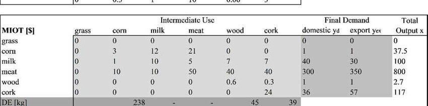
11Figure 2: PIOT, MIOT, and Leontief inverses for six-activity hypothetical economy
The hypothetical economy is represented by physical input-output table (PIOT) in kilograms (kg)
with corresponding Leontief inverse (I- AP)^-1 in kg/kg, vector of homogenous prices per product
in dollars per kilogram ($/kg), and monetary input-output table (MIOT) in dollars ($) with
corresponding Leontief inverse (I- AM)^-1 in $/$. Domestic extraction (DE) is the environmental
extension.
This hypothetical economy produces six commodities: grass, corn, milk, meat, wood, and cork.
Of these, four are extracted: Grass is grazed by the animals, corn is harvested in agriculture and
then used as animal feed, wood and cork are extracted in forestry operations. Milk and meat are
secondary products. In the PIOT, the total domestic extraction of grass, corn, wood, and cork
corresponds to the total output of these materials. Using a vector of homogenous prices, the
PIOT can be transformed into a MIOT. Note that grass has no direct market value. In material
12flow accounting (MFA) from which the indicator of domestic extraction (DE) stems, the
inclusion of materials as DE is not dependent on their market value and flows such as biomass
grazed by animals, used crop residues, and the surrounding rock in mined metal ores are also
accounted for. According to MFA conventions, animals, along with humans and artefacts, are
considered part of the socio-economic (rather than the natural) system so that their feed intake
from the natural system through grazing constitutes a form of domestic extraction (Fischer
Kowalski et al., 2011; OECD, 2007; Weisz et al., 2007).
For both the PIOT and the MIOT, we can construct the A matrices and calculate the Leontief
inverses following the procedure outlined in section 2. Because grass does not have a price, the
grass-producing sector is represented with zeroes in the MIOT and deleting this sector would
not change the subsequent calculations. In order to ensure that the grass DE is allocated in the
input-output system, it is necessary to allocate grass to another sector or to assign a (miniscule)
price to grass in constructing the MIOT, thereby creating a grass sector. The latter ensures that
the results based on the PIOT and MIOT calculations are identical (as we have seen in
Leontief’s example). Since PIOTs on which such a transformation could be based are hardly
available for real-world applications (see Weisz and Duchin, 2006), we present the former
alternative in Figure 2 and allocate grass in the same manner as corn as the only other vegetal
agricultural production represented.
Based on the Leontief inverses and our knowledge of final demand structure by domestic and
foreign final demand, we can calculate the direct and indirect material requirements associated
with final demand by type.
Figure 3: Material requirements associated with domestic and exported final demand (yd and
yex) in the hypothetical economy
Material requirements for each of the six commodities, as total, and as related to total final demand
(y), all units are kilograms (kg). The left two columns show the results as based on the physical input-
output table (PIOT) while the right two columns show the results based on the monetary input-output
model (MIOT).
Figure 3 shows the results of the environmental extension of our IO model both based on the
physical and the monetary IOT. In the PIOT-based model, the final demand for all six
commodities is associated with 162.53 kg of material requirements for domestic final demand
and 159.47 kg for exports, resulting in a total of 322 kg which corresponds to the total DE
included in our environmental extension (i.e. the total mass of grass, corn, wood, and cork). On
the other hand, the MIOT-based model yields different results: 161.18 kg of material
13requirements for domestic final demand and 160.82 kg for exports (322 kg in total
corresponding to total DE). If we had allocated grass by using a miniscule price, the results for
both the PIOT- and the MIOT-based approach would be identical. Assuming that grass can be
allocated like corn introduces a discrepancy between the PIOT- and the MIOT-based results.
The sum of all distributed materials is identical for both approaches (322 kg). If all goods have
market value and thus a (miniscule) price, the question is not if but how materials are allocated
using a material extension.
4. Call for Caution
EEIOA opens a wealth of economic data up to use within social ecology and constitutes an
attempt to specifically analyze structures of production and consumption and their material
requirements rather than assuming that materials flow through a societal black box. However,
some caveats in the application of this method unfortunately remain, as the issue of grass as a
non-market flow in our third example of a hypothetical economy (see section 3.2) already
suggests. Most of them circle around the fact that we do not (and probably will not) have reliable
physical input-output tables at our disposal so that we are forced to make some assumptions as
to how the flows recorded in the monetary input-output tables relate to the physical flows.
Input-output analysis is based on the assumption that product groups are homogenous, e.g. in
our hypothetical economy (Figure 2), we would have to assume that all corn is the same even
though different types of corn are used for food and feed. The IOT in our example covers flows
of fairly distinct products. In the real-life Austrian IOT, for example, all agricultural products
are reported in the same category (see Schaffartzik et al., 2014a). The more aggregated (i.e.,
lacking in detail) the product groups are, the greater their tendency to be homogenous. For many
economies, however, the available input-output tables aggregate very different products into
the same category (e.g. products of agriculture and forestry or of mining in the case of Austria
(Schaffartzik et al., 2014a)). Depending on how diverse the economic activities and the
associated material extraction in any one of these aggregate categories is for a given country,
the monetary data alone could lead to a contestable allocation of material flows within the IO
framework (Hubacek and Giljum, 2003; Suh, 2004; Weisz and Duchin, 2006; Wiedmann et al.,
2007). For example, if metal and fossil fuel mining are grouped into the same category,
domestic extraction of waste rock associated with metals mining would also find its way into
the fossil energy carrier supply chain. Because differences in level of sectoral aggregation lead
to differences in results (Miller and Blair, 2009), greater uncertainties are attached to the
material footprints of countries with a highly aggregated IOT as well as to the exports from
these countries.
The violation of homogenous prices as the second central assumption in input-output analysis
means that even results based on highly disaggregated tables are prone to bias. Different
economic activities may pay different prices for one and the same product; in terms of the IO
model this means that we have a matrix of prices rather than a vector (Merciai and Heijungs,
2014; Weisz and Duchin, 2006). In early energy analyses, it was already noted that energy is
not sold at the same price to all users. Primary industries, for example, generally pays less for
electricity than do service sectors or private households. This makes it preferable to use data in
physical units, i.e. in Joules (Bullard and Herendeen, 1975). Prices are the central mechanism
via which the integration of physical extension data into the input-output model can be
achieved. While Leontief illustrated his approach based on a physical input-output table (PIOT)
which he transformed into a MIOT using a vector of homogenous prices, reliable PIOTs are
14hardly available for modern-day IO applications (Weisz and Duchin, 2006). In the analysis of
material requirements, the differences in price of equivalent products will lead to errors in the
estimation. Whether a kg of bread costs 1 Euro or is of higher quality and costs 5 Euros, the
amount of crops required in the production of each will be roughly the same and certainly not
differ by a factor 5 as the price differences suggest (Kastner et al., 2013).
Monetary accounts do not include non-market flows which are used by society but have no
direct market value (grass in our example in Figure 2). Globally, the three most prominent flows
in material flow accounts in this category are grazed biomass and used crop residues as well as
waste rock extracted during mining activities. In 2010, these material flows accounted for 21%
of global domestic extraction (DE). In countries where mining and/or animal husbandry play
an important role, non-market flows make up more than half of material extraction (Giljum,
2004; Krausmann et al., 2008; Schaffartzik et al., 2014b). No standardized procedure exists for
the allocation of such non-market flows in the input-output model. For EEIOA-based accounts
of land embodied in trade flows (see, for example, Giljum et al., 2013; Lugschitz et al., 2011;
Steen-Olsen et al., 2012; Weinzettel et al., 2013; Wilting and Vringer, 2009; Yu et al., 2013),
non-market flows are crucial in assessing embodied pasture. Part of the difference in the results
generated by the aforementioned studies is due to the fact that they allocate grazing to different
economic activities (e.g. to cattle, raw milk, other animal products, or a combination of these).
How these assumptions are made strongly impacts the distribution of material flows that
currently account for 1/5 of global material extraction, affecting individual economies in a
disproportional manner.
Another long-standing issue in input-output applications pertains to the treatment of capital
stocks. Under the United Nations Systems of National Accounts on which input-output statistics
are based, gross capital formation, household consumption, and expenditures by government
and civic organizations are reported as categories of final demand (United Nations, 2003).
Capital can also be considered an input into (e.g. invested in machinery or factories) and
government spending (e.g. on infrastructure education) constitutes an indispensable basis for
production processes (Herendeen and Tanaka, 1976; Tukker and Jansen, 2006). National capital
accounts can be used to internalize investments into the intermediate use of each sector
(Hertwich, 2011; Lenzen, 2001; Lenzen and Treloar, 2004; Schoer et al., 2012). If this is done,
the results differ significantly from those of accounts in which investments are not internalized
(Minx et al., 2011; Schoer et al., 2012). Methodological decisions must then be made on their
depreciation: Allocating one year’s investments to that same year’s production ignores both
their role for future production and the role of past investments for current production. In a
study of global material consumption associated with final demand in the European Union,
Schoer and colleagues (2012) treat monetary depreciation of capital as sectoral inputs and
allocate net capital investments to the following years, with significant impacts on the results.
In the material extension of input-output models which is the focus of this article, the question
additionally arises whether depreciation rates applied to monetary capital are equally applicable
to physical stocks (e.g., buildings or machinery) (Pauliuk et al., 2014). These issues are decisive
in the interpretation of material footprints: The material inputs into production in mature
economies, using stocks accumulated over the past decades, is systematically lower than that
of emerging economies massively expanding their infrastructure and capital stocks (Müller et
al., 2013). For example, in-use stocks of steel in mature industrial economies are up to 5-10
times larger than in emerging and developing economies (Pauliuk et al., 2013).
Environmentally extended input-output analysis is undoubtedly a valuable tool not only within
social ecology but for sustainability science at large. As the EEIOA approach currently stands,
15however, we must exercise caution in interpreting results. Currently several research groups are
working on developing solutions to the remaining challenges. This will not only be helpful in
the interpretation and further analysis of EEIOA results but also in aiding us to better understand
the relationships between physical and monetary flows. For social ecology as the study of the
interrelations between the biophysical and the cultural, this corresponds to an important item
on the research agenda.
165. References
Ayres, R.U., Kneese, A.V., 1969. Production, consumption, and externalities. The American
Economic Review 59, 282–297.
Bullard, C.W., Herendeen, R.A., 1975. The energy cost of goods and services. Energy policy 3, 268–
278.
Daly, H.E., 1973. Towards a Steady-State Economics. WH Freeman, San Francisco, CA.
European Commission, 2011. A resource-efficient Europe–Flagship initiative under the Europe 2020
Strategy. COM (2011) 21.
Eurostat, 2008. Eurostat Manual of Supply, Use and Input-Output Tables, Methodologies and working
papers. Office for Official Publications of the European Communities, Luxembourg.
Fischer-Kowalski, M., Haberl, H., 1998. Sustainable development: socio economic metabolism and
colonization of nature. International Social Science Journal 50, 573–587.
Fischer Kowalski, M., Krausmann, F., Giljum, S., Lutter, S., Mayer, A., Bringezu, S., Moriguchi, Y.,
Schütz, H., Schandl, H., Weisz, H., 2011. Methodology and Indicators of Economy wide
Material Flow Accounting. Journal of Industrial Ecology 15, 855–876.
Fischer-Kowalski, M., Weisz, H., 1999. Society as hybrid between material and symbolic realms:
Toward a theoretical framework of society-nature interaction. Advances in Human Ecology 8,
215–252.
Giljum, S., 2004. Trade, Materials Flows, and Economic Development in the South: The Example of
Chile. Journal of Industrial Ecology 8, 241–261. doi:10.1162/1088198041269418
Giljum, S., Wieland, H., Bruckner, M., de Schutter, L., Giesecke, K., 2013. Land Footprint Scenarios:
A discussion paper including a literature review and scenario analysis on the land use related
to changes in Europe’s consumption patterns. Sustainable Europe Research Institute (SERI),
Vienna, Austria.
Herendeen, R., Tanaka, J., 1976. Energy cost of living. Energy 1, 165–178. doi:10.1016/0360-
5442(76)90015-3
Hertwich, E., 2011. The Life Cycle Environmental Impacts of Consumption. Economic Systems
Research 23, 27–47.
Hubacek, K., Giljum, S., 2003. Applying physical input–output analysis to estimate land appropriation
(ecological footprints) of international trade activities. Ecological Economics 44, 137–151.
Kastner, T., Schaffartzik, A., Eisenmenger, N., Erb, K.-H., Haberl, H., Krausmann, F., 2013. Cropland
area embodied in international trade: Contradictory results from different approaches.
Ecological Economics In Press. doi:10.1016/j.ecoloecon.2013.12.003
Krausmann, F., Erb, K.-H., Gingrich, S., Lauk, C., Haberl, H., 2008. Global patterns of socioeconomic
biomass flows in the year 2000: A comprehensive assessment of supply, consumption and
constraints. Ecological Economics 65, 471–487.
Lenzen, M., 2001. A Generalized Input–Output Multiplier Calculus for Australia. Economic Systems
Research 13, 65–92.
Lenzen, M., Treloar, G.J., 2004. Endogenising Capital: A comparison of Two Methods. Journal of
Applied Input-Output Analysis Vol. 10, 1–11.
Leontief, W., 1970. Environmental repercussions and the economic structure: an input-output
approach. The review of economics and statistics 52, 262–271.
Leontief, W.W., 1986. Input-output Economics. Oxford University Press.
Lugschitz, B., Bruckner, M., Giljum, S., 2011. Europe’s Global Land Demand: A study on the actual
land embodied in European imports and exports of agricultural and forestry products.
Sustainable Europe Research Institute (SERI), Vienna, Austria.
Meadows, D.H., Meadows, D.H., Randers, J., Behrens III, W.W., 1972. The Limits to Growth: A
Report to The Club of Rome (1972). Universe Books, New York.
Merciai, S., Heijungs, R., 2014. Balance issues in monetary input–output tables. Ecological
Economics 102, 69–74. doi:10.1016/j.ecolecon.2014.03.016
17Miller, R.E., Blair, P.D., 2009. Input-output analysis: foundations and extensions. Cambridge
University Press.
Minx, J.C., Baiocchi, G., Peters, G.P., Weber, C.L., Guan, D., Hubacek, K., 2011. A “Carbonizing
Dragon”: China’s Fast Growing CO2 Emissions Revisited. Environ. Sci. Technol. 45, 9144–
9153. doi:10.1021/es201497m
Müller, D.B., Liu, G., Løvik, A.N., Modaresi, R., Pauliuk, S., Steinhoff, F.S., Brattebø, H., 2013.
Carbon Emissions of Infrastructure Development. Environ. Sci. Technol. 47, 11739–11746.
doi:10.1021/es402618m
OECD, 2007. Measuring Material Flows and Resource productivity – OECD guidance manual.
Volume II: A theoretical framework for material flow accounts and their applications at
national level. Working Group on Environmental Information and Outlooks, Organisation for
Economic Co-operation and Development (OECD), Paris.
Pauliuk, S., Wang, T., Müller, D.B., 2013. Steel all over the world: Estimating in-use stocks of iron for
200 countries. Resources, Conservation and Recycling 71, 22–30.
doi:10.1016/j.resconrec.2012.11.008
Pauliuk, S., Wood, R., Hertwich, E.G., 2014. Dynamic Models of Fixed Capital Stocks and Their
Application in Industrial Ecology. Journal of Industrial Ecology n/a–n/a.
doi:10.1111/jiec.12149
Rockström, J., Steffen, W., Noone, K., Persson, Å., Chapin, F.S., Lambin, E.F., Lenton, T.M.,
Scheffer, M., Folke, C., Schellnhuber, H.J., Nykvist, B., de Wit, C.A., Hughes, T., van der
Leeuw, S., Rodhe, H., Sörlin, S., Snyder, P.K., Costanza, R., Svedin, U., Falkenmark, M.,
Karlberg, L., Corell, R.W., Fabry, V.J., Hansen, J., Walker, B., Liverman, D., Richardson, K.,
Crutzen, P., Foley, J.A., 2009. A safe operating space for humanity. Nature 461, 472–475.
doi:10.1038/461472a
Schaffartzik, A., Eisenmenger, N., Krausmann, F., Weisz, H., 2014a. Consumption-based Material
Flow Accounting: Austrian trade and consumption in raw material equivalents 1995-2007.
Journal of Industrial Ecology 18, 102–112. doi:10.1111/jiec.12055
Schaffartzik, A., Mayer, A., Gingrich, S., Eisenmenger, N., Loy, C., Krausmann, F., 2014b. The
global metabolic transition: Regional patterns and trends of global material flows, 1950–2010.
Global Environmental Change 26, 87–97. doi:10.1016/j.gloenvcha.2014.03.013
Schoer, K., Weinzettel, J., Kovanda, J., Giegrich, J., Lauwigi, C., 2012. Raw Material Consumption of
the European Union – Concept, Calculation Method, and Results. Environ. Sci. Technol. 46,
8903–8909. doi:10.1021/es300434c
Steen-Olsen, K., Weinzettel, J., Cranston, G., Ercin, A.E., Hertwich, E.G., 2012. Carbon, Land, and
Water Footprint Accounts for the European Union: Consumption, Production, and
Displacements through International Trade. Environ. Sci. Technol. 46, 10883–10891.
doi:10.1021/es301949t
Suh, S., 2004. A note on the calculus for physical input–output analysis and its application to land
appropriation of international trade activities. Ecological Economics 48, 9–17.
Tukker, A., Jansen, B., 2006. Environmental impacts of products: A detailed review of studies. Journal
of Industrial Ecology 10, 159–182.
United Nations, 2003. National Accounts: A Practical Introduction, Studies in Methods: Handbook of
National Accounting. UN Department of Economic and Social Affairs, Statistics Division,
United Nations, New York.
Weinzettel, J., Hertwich, E.G., Peters, G.P., Steen-Olsen, K., Galli, A., 2013. Affluence drives the
global displacement of land use. Global Environmental Change.
Weisz, H., Duchin, F., 2006. Physical and monetary input–output analysis: What makes the
difference? Ecological Economics 57, 534–541.
Weisz, H., Krausmann, F., Eisenmenger, N., Schütz, H., Haas, W., Schaffartzik, A., 2007. Economy-
wide material flow accounting. A compilation guide. Eurostat and the European Commission.
Wiedmann, T., Lenzen, M., Turner, K., Barrett, J., 2007. Examining the global environmental impact
of regional consumption activities—Part 2: Review of input–output models for the assessment
of environmental impacts embodied in trade. Ecological Economics 61, 15–26.
18Wilting, H.C., Vringer, K., 2009. Carbon and land use accounting from a producer’s and a consumer’s
perspective - an empirical examination covering the world. Economic Systems Research 21,
291–310. doi:10.1080/09535310903541736
Yu, Y., Feng, K., Hubacek, K., 2013. Tele-connecting local consumption to global land use. Global
Environmental Change 23, 1178–1186. doi:10.1016/j.gloenvcha.2013.04.006
19WORKING PAPERS SOCIAL ECOLOGY
Band 1 Band 13
Umweltbelastungen in Österreich als Folge mensch- Transportintensität und Emissionen. Beschreibung
lichen Handelns. Forschungsbericht gem. m. dem Öster- österr. Wirtschaftssektoren mittels Input-Output-Mo-
reichischen Ökologie-Institut. Fischer-Kowalski, M., Hg. dellierung. Forschungsbericht gem. m. dem Österr.
(1987) Ökologie-Institut. Dell'Mour, R.; Fleissner, P.; Hofkirchner,
W.; Steurer, A. (1991)
Band 2
Environmental Policy as an Interplay of Professionals Band 14
and Movements - the Case of Austria. Paper to the ISA Indikatoren für die Materialintensität der öster-
Conference on Environmental Constraints and Opportu- reichischen Wirtschaft. Forschungsbericht gem. m. dem
nities in the Social Organisation of Space, Udine 1989. Österreichischen Ökologie-Institut. Payer, H. unter Mitar-
Fischer-Kowalski, M. (1989) beit von K. Turetschek (1991)
Band 3 Band 15
Umwelt &Öffentlichkeit. Dokumentation der gleichnami- Die Emissionen der österreichischen Wirtschaft. Syste-
gen Tagung, veranstaltet vom IFF und dem Österreichi- matik und Ermittelbarkeit. Forschungsbericht gem. m.
schen Ökologie-Institut in Wien, (1990) dem Österr. Ökologie-Institut. Payer, H.; Zangerl-Weisz,
H. unter Mitarbeit von R.Fellinger (1991)
Band 4
Umweltpolitik auf Gemeindeebene. Politikbezogene Band 16
Weiterbildung für Umweltgemeinderäte. Lackner, C. Umwelt als Thema der allgemeinen und politischen
(1990) Erwachsenenbildung in Österreich. Fischer-Kowalski M.,
Fröhlich, U.; Harauer, R.; Vymazal, R. (1991)
Band 5
Verursacher von Umweltbelastungen. Grundsätzliche Band 17
Überlegungen zu einem mit der VGR verknüpfbaren Causer related environmental indicators - A contribution
Emittenteninformationssystem. Fischer-Kowalski, M., to the environmental satellite-system of the Austrian
Kisser, M., Payer, H., Steurer A. (1990) SNA. Paper for the Special IARIW Conference on Envi-
ronmental Accounting, Baden 1991. Fischer-Kowalski, M.,
Band 6 Haberl, H., Payer, H., Steurer, A. (1991)
Umweltbildung in Österreich, Teil I: Volkshochschulen.
Fischer-Kowalski, M., Fröhlich, U.; Harauer, R., Vymazal R. Band 18
(1990) Emissions and Purposive Interventions into Life Pro-
cesses - Indicators for the Austrian Environmental Ac-
Band 7 counting System. Paper to the ÖGBPT Workshop on
Amtliche Umweltberichterstattung in Österreich. Fischer- Ecologic Bioprocessing, Graz 1991. Fischer-Kowalski M.,
Kowalski, M., Lackner, C., Steurer, A. (1990) Haberl, H., Wenzl, P., Zangerl-Weisz, H. (1991)
Band 8 Band 19
Verursacherbezogene Umweltinformationen. Bausteine Defensivkosten zugunsten des Waldes in Österreich.
für ein Satellitensystem zur österr. VGR. Dokumentation Forschungsbericht gem. m. dem Österreichischen Insti-
des gleichnamigen Workshop, veranstaltet vom IFF und tut für Wirtschaftsforschung. Fischer-Kowalski et al.
dem Österreichischen Ökologie-Institut, Wien (1991) (1991)
Band 9 Band 20*
A Model for the Linkage between Economy and Envi- Basisdaten für ein Input/Output-Modell zur Kopplung
ronment. Paper to the Special IARIW Conference on ökonomischer Daten mit Emissionsdaten für den Be-
Environmental Accounting, Baden 1991. Dell'Mour, R., reich des Straßenverkehrs. Steurer, A. (1991)
Fleissner, P. , Hofkirchner, W.,; Steurer A. (1991)
Band 22
Band 10 A Paradise for Paradigms - Outlining an Information
Verursacherbezogene Umweltindikatoren - Kurzfassung. System on Physical Exchanges between the Economy
Forschungsbericht gem. mit dem Österreichischen and Nature. Fischer-Kowalski, M., Haberl, H., Payer, H.
Ökologie-Institut. Fischer-Kowalski, M., Haberl, H., Payer, (1992)
H.; Steurer, A., Zangerl-Weisz, H. (1991)
Band 23
Band 11 Purposive Interventions into Life-Processes - An Attempt
Gezielte Eingriffe in Lebensprozesse. Vorschlag für to Describe the Structural Dimensions of the Man-
verursacherbezogene Umweltindikatoren. For- Animal-Relationship. Paper to the Internat. Conference
schungsbericht gem. m. dem Österreichischen Öko- on "Science and the Human-Animal-Relationship", Am-
logie-Institut. Haberl, H. (1991) sterdam 1992. Fischer-Kowalski, M., Haberl, H. (1992)
Band 12 Band 24
Gentechnik als gezielter Eingriff in Lebensprozesse. Purposive Interventions into Life Processes: A Neg-
Vorüberlegungen für verursacherbezogene Umweltindi- lected "Environmental" Dimension of the Society-Nature
katoren. Forschungsbericht gem. m. dem Österr. Ökolo- Relationship. Paper to the 1. Europ. Conference of Soci-
gie-Institut. Wenzl, P.; Zangerl-Weisz, H. (1991) ology, Vienna 1992. Fischer-Kowalski, M., Haberl, H. (1992)You can also read