Data-SUITE: Data-centric identification of in-distribution incongruous examples - arXiv
←
→
Page content transcription
If your browser does not render page correctly, please read the page content below
Data-SUITE: Data-centric identification of in-distribution
                                                            incongruous examples
                                                    Nabeel Seedat∗1 , Jonathan Crabbe1 , and Mihaela van der Schaar1,2,3
                                                                                     1
                                                                                  University of Cambridge
arXiv:2202.08836v2 [cs.LG] 18 Feb 2022

                                                                                 2
                                                                                 The Alan Turing Institute
                                                                     3
                                                                       University of California, Los Angeles (UCLA)

                                                                                            Abstract
                                                    Systematic quantification of data quality is critical for consistent model performance. Prior
                                                works have focused on out-of-distribution data. Instead, we tackle an understudied yet equally
                                                important problem of characterizing incongruous regions of in-distribution (ID) data, which may
                                                arise from feature space heterogeneity. To this end, we propose a paradigm shift with Data-
                                                SUITE: a data-centric framework to identify these regions, independent of a task-specific model.
                                                DATA-SUITE leverages copula modeling, representation learning, and conformal prediction to
                                                build feature-wise confidence interval estimators based on a set of training instances. These
                                                estimators can be used to evaluate the congruence of test instances with respect to the training
                                                set, to answer two practically useful questions: (1) which test instances will be reliably predicted
                                                by a model trained with the training instances? and (2) can we identify incongruous regions
                                                of the feature space so that data owners understand the data’s limitations or guide future
                                                data collection? We empirically validate Data-SUITE’s performance and coverage guarantees
                                                and demonstrate on cross-site medical data, biased data, and data with concept drift, that
                                                Data-SUITE best identifies ID regions where a downstream model may be reliable (independent
                                                of said model). We also illustrate how these identified regions can provide insights into datasets
                                                and highlight their limitations.

                                         1      Introduction
                                         Machine learning models have a well-known reliance on training data quality [Park et al., 2021].
                                         Hence, when deploying such models in the real world, the reliability of predictions depends on the
                                         data’s congruence with respect to the training data. Significant literature has focused on identifying
                                         data instances that lie out of the training data’s distribution (OOD). This includes label shifts [Ren
                                         et al., 2018, Hsu et al., 2020] or input feature shift where these instances fall out of the support of the
                                         training set’s distribution [Zhang et al., 2021]. However, a much less studied yet equally important
                                         problem is identifying heterogeneous regions of in-distribution (ID) data.
                                         Data in the wild can be ID yet have heterogeneous regions in feature space. This manifests in varying
                                         levels of incongruence, in cases of different sub-populations, data biases or temporal changes [Leslie
                                         et al., 2021, Gianfrancesco et al., 2018, Obermeyer et al., 2019]. We illustrate each of these types of
                                         incongruence with real world data (Table 2), in the experiments from Sections 4.3 and 4.4.
                                         In this paper, we present a data-centric framework to characterize such incongruous regions of ID
                                         data and define two groups, namely, (i) inconsistent and (ii) uncertain, with respect to the training
                                             ∗ Corresponding   author: ns741@cam.ac.uk

                                                                                                 1
(a) ALICE (D1):                                                                     (b) BOB (D2):
          Data Exploration                                                                    Model Deployment

                                                         Feature 1 Feature 2   UNCERTAIN                  Instance 1
                                              Sample 1                         INSTANCES
                                              Sample 2                                        Feature 1
                                                                               (Large CIs)
                                                                                              Feature 2
                                                         Feature 1 Feature 2   INCONSISTENT                             Predicted Value     +
                                              Sample 1                         INSTANCES      Feature 3                 Predictive uncertainty
                                              Sample 2
                                                                               (Outside CI)
                                                         Feature 1 Feature 2   CERTAIN        Data-Centric             Model-Centric
                                              Sample 1                         INSTANCES       Uncertainty              Uncertainty
                        Out-of-distribution
                                              Sample 2                         (Small CIs)       (Model                   (Model
                        (OOD)                                                                 Independent)              Dependent)
                                                   In-distribution (ID)

                Figure 1: Illustration highlighting two problems Data-SUITE addresses

distribution. We contextualize the difference based on confidence intervals (CI) (See Sec.3.3 for
details). When feature values lie outside of a CI, we term it inconsistent, alternatively we characterize
the level of feature uncertainty based on the CI’s width.
At this point one might ask if the data is ID; why should we worry? Not accounting for these
incongruous ID regions of the feature space can be problematic when deploying models in high-
stakes settings such as healthcare, where spurious model predictions can be deadly [Saria and
Subbaswamy, 2019, Varshney, 2020]. That said, even in settings where poor predictions are not risky,
consistent exploratory data analysis (EDA) and retroactive auditing of such data is time-consuming
for data scientists [Polyzotis et al., 2017, Kandel et al., 2012]. Hence, systematically identifying these
incongruous regions has immense practical value.
Consequently, we build a framework to empower data scientists to address the previously mentioned
challenges related to insightful exploratory data analysis (EDA) and reliable model deployment,
anchored by the following desiderata:
(D1) Insightful Data Exploration: Alice has a new dataset D and wants to explore and gain
insights into it with respect to a training set, without necessarily training a model. It would be
useful if, independent of a predictive model, she could both identify the incongruous regions of the
feature space (e.g., sub-population bias or under-representation), as well as, obtain easily digestable
prototype examples of each region. This could guide where to collect more data and if this is not
possible, to understand the data’s limitations.
(D2) Reliable Model Deployment: Bob has a trained model f ∗ and now deploys it to another
site. For new data Dtest , it would be useful if he could identify incongruous regions, for which he
should NOT trust f ∗ to make predictions.
(D3) Practitioner confidence: Both Alice and Bob want to feel confident when using any tool.
Guarantees of coverage of predictive intervals (e.g. CIs) could assist in this regard.
These examples, shown in Fig. 1 highlight the need to understand incongruence in data. As we
shall discuss in the related work, there has been significant work on uncertainty estimation, with a
focus on the uncertainty of a model’s predictions (model-centric). Estimating predictive uncertainty
can address Bob’s use-case (D2 ), however since it requires a predictive model it is not naturally
suited to Alice’s insights use-case (D1 ). Further, most predictive uncertainty methods do not provide
guarantees on coverage (D3 ).
Therefore, in satisfying all the desiderata, we take a different approach and advocate for modeling the
uncertainty in the data features 1 . This is different from model predictive uncertainty, as we construct
  1 Here, “feature” uncertainty refers to the degree of incongruity with the training distribution, rather than the

uncertainty of the measured value (e.g. measurement noise)

                                                                               2
CIs (at feature level), without reference to any downstream model. A benefit of the flexibility is that
we can flag instances and draw insights that are not model-specific (i.e. model independent). We
focus on tabular data, a common format in medicine, finance, manufacturing etc, where data is based
on relational databases [Borisov et al., 2021, Yoon et al., 2020]. That said, compared to image data,
tabular data has an added challenge since specific features may be uncertain while others are not;
hence characterizing an instance as a whole is non-trivial.

Contributions. We present Data Searching for Uncertain and Inconsistent Test Examples (Data-
SUITE), a data-centric framework to identify incongruous regions of data using CI’s and make the
following contributions:
• Data-SUITE is a paradigm shift from model-centric uncertainty and, to the best of our knowledge,
the first to characterize ID regions in a systematic data-centric, model-independent manner. Not
only is this more flexible but also enables us to gain insights which are not model-specific.
• Data-SUITE’s pipeline-based approach to construct feature-wise CIs enables specific properties
(Sec. 3.2) that permit us to flag uncertain and inconsistent instances, making it possible to identify
incongruous data regions.
• Data-SUITE’s performance and properties, such as coverage guarantees are validated to satisfy D3
(Sec. 4.1).
• Further motivating the paradigm shift, we empirically highlight the performance benefit of a
data-centric approach compared to a model-centric approach (Sec. 4.2).
• As a portrayal of reliable model deployment (D2 ), we show on real-world datasets with different
types of incongruence, that Data-SUITE best identifies incongruous data regions, translating to the
best performance improvement. (Sec. 4.3).
• Finally, we illustrate with multiple use-cases how Data-SUITE can be used as a model-independent
tool to facilitate insightful data exploration, hence satisfying D1 (Sec. 4.4).

2    Related work
This paper primarily engages with the literature on uncertainty quantification and contributes to the
nascent area of data-centric ML. We also highlight key differences of our work to the literature on
noisy labels.
Uncertainty quantification. There are numerous Bayesian and non-Bayesian methods proposed
for uncertainty quantification, including Gaussian processes [Williams and Rasmussen, 2006], Quantile
Regression [Koenker and Hallock, 2001], Bayesian Neural Networks [Ghosh et al., 2018, Graves, 2011],
Deep Ensembles [Lakshminarayanan et al., 2017], MC Dropout [Gal and Ghahramani, 2016] and
Conformal Prediction [Vovk et al., 2005, Balasubramanian et al., 2014]. These methods typically
model predictive uncertainty, i.e., measuring the certainty in the model’s prediction. The predominant
focus on predictive uncertainty is different from the notion of uncertainty in our setting, which
is feature (i.e. data) uncertainty. We specifically highlight that we quantify data uncertainty,
independent of a task-specific model. Additionally, the aforementioned methods often do not assess
the coverage or provide guarantees of the uncertainty interval [Wasserman, 2004] (i.e., how often the
interval contains the true value). The concept of coverage will be outlined further in Sections 3 and 4.
Data-Centric ML. Ensuring high data quality is a critical but often overlooked problem in ML,
where the focus is optimizing models [Sambasivan et al., 2021, Jain et al., 2020]. Even when it is
considered, the process of assessing datasets is adhoc or artisinal [Sambasivan et al., 2021, Ng et al.,
2021]. However, there has been recent discussion around data-centric ML, which involves tools applied
to the underlying data used to train and evaluate models, independent of the task-specific, predictive
models. Our work contributes to this nascent body of work - presenting Data-SUITE, which, to the
best of our knowledge, is the first systematic data-centric framework to model uncertainty in datasets.

                                                   3
Specifically, we model the uncertainty in the feature (data) values themselves (data-centric), which
contrasts modeling the uncertainty in predictions (model-centric).
Noisy labels. Learning with noisy data is a widely studied problem, we refer the reader to [Algan
and Ulusoy, 2021, Song et al., 2020] for an in depth review. In the machine learning context, there is
a focus on label noise. We argue that work on noisy labels is not directly related, as the typical goal is
to learn a model robust to the label noise, which is different from our goal of modeling the uncertainty
in the features. Additionally, the success of the literature on noisy labels is tightly coupled to the
task-specific predictive model, which is different from our model-independent setting.

3     Data-SUITE
In this section, we give a detailed formulation of Data-SUITE. We start with a problem formulation
and outline the motivation for working with feature confidence intervals (CIs). Then, we describe how
these CIs are built by leveraging copula modelling, representation learning and conformal prediction.
Finally, we demonstrate how these CIs permit to flag uncertain and inconsistent instances.

3.1     Preliminaries
                                   QdX
We consider a feature space X = i=1    [ai , bi ] ⊆ RdX , where [ai , bi ] is the range for feature i. Note
that we make the range of each feature explicit, this will be necessary in the definition of our
formalism. We assume that we have a set of M ∈ N∗ training instances Dtrain = {xm | m ∈ [M ]}
sampled from an unknown distribution P, where [M ] denotes the positive integers between 1 and
M . These instances typically correspond to training data for a model on a downstream task such as
classification.
We assume that we are given new test instances Dtest . Our purpose is to flag the subset of instances
from Dtest that are quantitatively different from instances of Dtrain without necessarily being OOD.
To that aim, we use Dtrain to build CIs [li (x), ri (x)] ⊆ [ai , bi ] for each feature i ∈ [dX ] of each test
instance x ∈ Dtest . As we will show in Section 3.3, these CIs permit to systematically flag test
instances whose features are uncertain or inconsistent with respect to Dtrain . For now, let us motivate
the usage of feature CIs: (1) With a model of uncertainty and inconsistency at the feature level, it
is possible to identify regions of the feature space X where bias and/or low coverage occurs with
the training data Dtrain . (2) Since CIs are built with Dtrain and without reference to any predictive
downstream model, the flagged instances in Dtest are likely to be problematic for any downstream
model trained on top of Dtrain . Hence, we are able to draw conclusions that are not model-specific.
These two points are illustrated in our experiments from Section 4. Let us now detail how the CIs
are built.

3.2     Feature CIs
We now build CIs [li (x), ri (x)] ⊆ [ai , bi ] for each feature i ∈ [dX ] of each test instance x ∈ Dtest . It
goes without saying that the CIs should satisfy some properties, i.e.
(P1) Coverage: We would like to guarantee         that the feature xi of an instance x ∼ P lies within the
interval such that E 1xi ∈[li (x),ri (x)] ≥ 1 − α where the significance level α ∈ (0, 1) can be chosen. In


this way, a feature out of the CI hints that x is unlikely to be sampled from P at the given significance
level. This is then considered across all features to characterize the instance (see Section 3.3).
(P2) Instance-wise: The CI should be adaptive at an instance level. i.e, we do not wish ri (x) − li (x)
to be constant w.r.t x ∈ X . In this way, the CIs permit to order various test instances x ∈ Dtest
according to their uncertainty. This property is particularly desirable in healthcare settings where we
wish to quantify variable uncertainty for individual patients, rather than for a population as whole.
(P3) Feature-wise: We build CIs [li (x), ri (x)] for each feature i ∈ [dX ] as opposed to an overall

                                                      4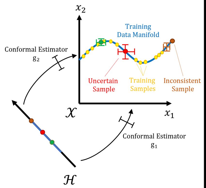
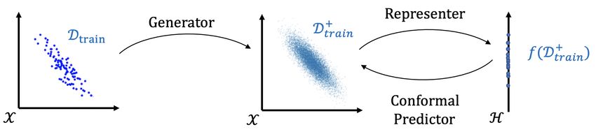
Figure 2: Outline of our framework Data-SUITE.

confidence region R(x) ⊂ X . While less general that the latter approach, feature-wise CIs are more
interpretable, allowing attribution of inconsistencies and uncertainty to individual features.
(P4) Downstream coupling: Instances with smaller CIs are more reliably predicted by a downstream
model trained on Dtrain . More precisely, our CIs should have a negative correlation between CI
width and downstream model performance. In this way, CIs allow to draw conclusions about the
incongruence of test instances x ∈ Dtest .
To construct feature CIs that satisfy these properties, we introduce a new framework leveraging
copula modeling, representation learning and conformal prediction. The blueprint of our method is
presented in Fig. 2. Concretely, our method relies on 3 building blocks: a generator that augments
the initial training set Dtrain ; a representer that leverages the augmented training set Dtrain
                                                                                            +
                                                                                                 to learn
a low-dimensional representation f : X → H of the data and a conformal predictor that predicts
instance-wise feature CIs [li (x), ri (x)] on the basis of each instance’s representation f (x) ∈ H. By
construction, this method fulfills properties (P2) and (P3). As we will see in the following, the
conformal predictor guarantees (P1). We demonstrate (P4) empirically in Section 4. Appendix C.1
quantifies the significance of each block via an ablation study. Let us now detail each block.

Generator. The purpose of the generator is to augment the initial training set Dtrain with instances
that are consistent with the initial distribution P. Many data augmentation techniques can be used
for this block. Since our focus is on tabular data, we found copula modeling to be particularly useful.
Copulas leverage Sklar’s theorem [Sklar, 1959] to estimate multivariate distributions with univariate
marginal distributions. In our case, we use vine copulas [Bedford and Cooke, 2001] to build an
estimate P̂ for the distribution P on the basis of Dtrain . We then build an augmented training set
  +
Dtrain by sampling from the copula density P̂. Interestingly, our method does not need to access
Dtrain once the copula density P̂ is available. It is perfectly possible to use only instances from P̂
to build the augmented dataset Dtrain +
                                         . This could be useful for data sharing, if the access to the
training set Dtrain is restricted to the user. Further details and motivations on copulas is found in
Appendix A.2.1. Note that a copula might not be ideal for very high-dimensional (large dX ) data in
domains such as computer vision or genomics. In those cases, copula modeling can be replaced by
domain-specific augmentation techniques.

Representer. A trivial way to verify the coverage guarantee (P1) would be to use the true values
of the features to build the CIs: [li (x), ri (x)] = [xi − δ, xi + δ] for some δ ∈ R+ . The problem with
this approach is two-fold: (1) it does not leverage the distribution P underlying the training set Dtrain
and (2) it results in an uninformative reconstruction with CIs that do not capture the specificity
of each instance, hence contradicting (P2). To provide a more satisfactory solution, we propose to
represent the augmented training data Dtrain  +
                                                   with a representation function f : X → H that maps
the data into a lower-dimensional latent representation space H ⊆ RdH , dH < dX . The purpose of
this representer is to capture the structure of the low-dimensional manifold underlying Dtrain
                                                                                             +
                                                                                                 . At test

                                                    5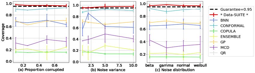
time, the conformal predictor (detailed next), uses the lower representations f (x) ∈ H to estimate a
reconstruction interval for each feature xi . This permits to bring a satisfactory solution to the two
aforementioned problems: (1) the CIs are reconstructed in terms of latent factors that are useful
to describe the training set Dtrain and (2) the predicted CIs vary according to the representation
f (x) ∈ H of each test instance x ∈ Dtest . In essence, our approach is analogous to autoencoders. As
we will explain soon, the crucial difference is the decoding step: our method outputs CIs for the
reconstructed input. In this work, we use Principal Component Analysis (PCA), the workhorse for
tabular data, to learn the representer f . Note that more general encoder architectures can be used
in relevant settings such as computer vision.

Conformal Predictor. We now turn to the core of the problem: estimating feature-wise CIs.
As previously mentioned, the CIs [li (x), ri (x)], i ∈ [dX ] will be computed on the basis of the latent
representation f (x) for each x ∈ Dtest . The idea is simple: for each feature i ∈ [dX ], we train
a regressor gi : H → [ai , bi ] to reconstruct an estimate of the initial features xi from the latent
representation f (x) of the associated training instance: (gi ◦ f )(x) ≈ xi . We stress that the regressor
gi has no knowledge of the true observed xi but only of the latent representation f (x), as illustrated
in Fig. 3. Of course, the feature regressor by themselves provide point-wise estimates for the features.
In order to turn these into CIs, we use conformal prediction as a wrapper around the feature
regressor [Vovk et al., 2005].

                          Figure 3: Conformal Predictor in Data-SUITE.

In practice, we formalize our problem in the framework of Inductive Conformal Prediction (for
motivations see Appendix A.2.2). Hence, under the formulation, we start by splitting the augmented
training set into a proper training set and a calibration set: Dtrain
                                                                   +         +
                                                                        = Dtrain2      +
                                                                                   t Dcal . We use the
latent representation of the proper training set, to train the feature regressor gi , i ∈ [dX ] for the
reconstruction task. Then, the latent representation of the calibration set is used to compute the
non-conformity score (µ), which estimates how different a new instance looks from other instances.
In practice, we use the absolute error non-conformity score µi (x) = |xi − (gi ◦ f )(x)|. We obtain an
empirical distribution of non-conformity scores {µi (x) | x ∈ Dcal
                                                               +
                                                                   } over the calibration instances for

                                                    6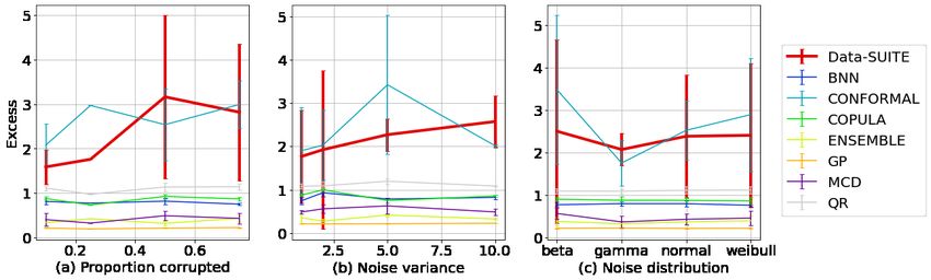
each feature i ∈ [dX ]. This is used to obtain the critical non-conformity score , which corresponds
to the d(|Dcal +
                  | + 1)(1 − α)e-th smallest residual from the set {µi (x) | x ∈ Dcal +
                                                                                        } [Vovk, 2013]. We
then apply the method to any unseen incoming data to obtain predictive CIs for the data point
i.e. [li (x), ri (x)] = [(gi ◦ f )(x) − , (gi ◦ f )(x) + ]. However, in this form the CIs are constant for
all instances, where the width of the interval is determined by the residuals of the most difficult
instances (largest residuals).
We adapt our conformal prediction framework to obtain the desired adaptive intervals (P2 ) using
a normalized non-conformity function (γ), see Eq. 1 [Boström et al., 2016, Johansson et al., 2015].
The numerator is computed as before based on µ, however, the denominator normalizes per instance.
We learn the normalizer per feature i ∈ [dX ].
To do so, we compute the log residuals per feature, for all instances in the respective proper training
set Dtrain2 . We produce tuples per feature: {(f (x), ln|x − (gi ◦ f )(x)|) | x ∈ Dtrain2 }. These are
used to train a different model, σi : X → R+ (e.g., MLP), to predict the log residuals. We can
then apply σi to test instances to capture the difficulty in predicting said instance. Note, we apply
an exponential to the predicted log residual for the test instance converting to the true scale and
ensuring positive estimates.
                                                       |xi − (gi ◦ f )(x)|
                                            γi (x) ≡                       ,                             (1)
                                                             σi (x)
We can then obtain the critical non-conformity score  applied to the empirical distribution of
normalized non-conformity scores {γi (x) | x ∈ Dcal
                                                +
                                                    }, in the same way as before based on residuals.
The instance-specific adaptive intervals are then obtained as per Eq. 2, where g is the underlying
feature regressor and σi is the instance-wise normalizing function.

                           [li (x), ri (x)] = [(gi ◦ f )(x) − σi (x), (gi ◦ f )(x) + σi (x)]           (2)

Remarks on theoretical guarantees. Under the exchangeability assumption detailed in the
Appendix A.2.2, the validity of coverage guarantees (P2) is fulfilled with our definition. In our
implementation, we use α = .05.

3.3       Identifying Inconsistent and Uncertain Instances
Now that we have CIs [li (x), ri (x)] ⊂ [ai , bi ] for each feature xi , i ∈ [dX ] of the instance x, we can
evaluate if instances from a dataset falls within the predicted range. If it falls outside the predicted
range we characterize the inconsistency (see Definition 1)
Definition 1 (Inconsistency). Let x ∈ Dtest be a test instance for which we construct a (1 − α)-CI,
[li (x), ri (x)], for each feature xi , i ∈ [dX ] for some predetermined α ∈ (0, 1). For each xi , i ∈ [dX ],
the feature inconsistency is a binary variable indicating if xi falls out of the CI.
                                           νi (x) ≡ 1(xi ∈
                                                         / [li (x), ri (x)])                             (3)
The instance inconsistency ν(x) is obtained by averaging over the feature inconsistencies νi (x).
                                                            dX
                                                          1 X
                                                ν(x) ≡          νi (x)
                                                         dX i=1

The instance x is inconsistent if the fraction of inconsistent features is above a predetermined
threshold2 λ ∈ [0, 1]: ν(x) > λ.
  2 In   our implementation, we use λ = 0.5.

                                                           7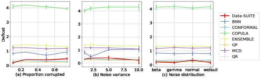
There can also be degrees of uncertainty in the feature value for features that fall within the CI,
which can reflect the instance as a whole. Indeed, if the CI [li (x), ri (x)] is large, the feature xi is
likely to fall within its range. Nonetheless, we should keep in mind that large CIs correspond to a
large uncertainty for the related feature. This will also typically happen when the instance x ∈ Dtest
differs from the training set Dtrain used to build the CI. We now introduce a quantitative measure
that expresses the degree of uncertainty of the instance with respect to Dtrain (see Definition 2).
Definition 2 (Uncertainty). Let x ∈ Dtest be a test instance for which we construct a (1 − α) CI
[li (x), ri (x)] for each feature xi , i ∈ [dX ] for some predetermined α ∈ (0, 1). For each xi , i ∈ [dX ], we
define the feature uncertainty ∆i (x) as the feature CI width normalized by the feature range:

                                                      ri (x) − li (x)
                                           ∆i (x) ≡                                                        (4)
                                                          bi − ai
The instance uncertainty ∆(x) is obtained by averaging over all feature uncertainties:
                                                  dX
                                                1 X
                                      ∆(x) ≡          ∆i (x) ∈ (0, 1].
                                               dX i=1

Remark 1. Instance uncertainties are strictly larger than zero as feature uncertainties are computed
over all features. Hence, this characterization offers a natural split between certain and uncertain
instances if we sort the instances based on uncertainty.

4     Experiments
This section presents detailed empirical evaluation demonstrating that Data-SUITE satisfies (D1)
Insightful Data Exploration,(D2) Reliable Model Deployment and (D3) Practitioner confidence,
introduced in Section 1. We tackle these in reverse order as practitioner confidence is a prerequisite
for the adoption of D1 and D2.
Recall that the notion of uncertainty in Data-SUITE is different from predictive uncertainty (model-
centric). We empirically compare these two paradigms using methods for predictive uncertainty.
That said, a natural additional question is whether model-centric uncertainty estimation methods
can simply be applied to this setting and provide uncertainty estimates for feature values.
We benchmark the following widely used Bayesian and non-Bayesian methods (under BOTH the
model-centric & data-centric paradigms): Bayesian Neural Networks (BNN) [Ghosh et al., 2018],
Deep Ensembles (ENS) [Lakshminarayanan et al., 2017], Gaussian Processes (GP) [Williams and
Rasmussen, 2006], Monte-Carlo Dropout (MCD) [Gal and Ghahramani, 2016] and Quantile Regression
(QR) [Koenker and Hallock, 2001]. We also ablate and test Data-SUITE’s constituent components
independently: conditional sampling from copula (COP), Conformal Prediction on raw data (CONF)
[Vovk et al., 2005, Balasubramanian et al., 2014]. For implementation details see Appendix B.1.

4.1    Validating coverage & comparing properties
We firstly wish to validate the CIs to ensure that the coverage guarantees are satisfied such that
users can have confidence that the true value lies within the predicted CIs (D3). We assess the CIs
based on the following metrics defined in [Navratil et al., 2020] - (1) Coverage: how often the CI
contains the true value, (2) Deficit: extent of CI shortfall (i.e., the severity of the errors) and (3)
Excess: extent of CI excess width to capture the true value.

                                                       8
Coverage = E 1xi ∈[li ,ri ] (5)
Deficit = E 1xi ∈[l (6)
/ i ,ri ] · min {|xi − li | , |xi − ri |}
Excess = E 1xi ∈[li ,ri ] · min {xi − li , ri − xi } (7)
Synthetic data. We assess the properties of different methods using synthetic data as the ground
truth values are available, even when encoding incongruence. The synthetic data with features,
X = [X1 , X2 , X3 ], is drawn IID from a multivariate
P Gaussian distribution, parameterized by mean
vector µ and a positive definite covariance matrix (details in Appendix B.2). We sample n = 1000
synth synth synth
points for both Dtrain and Dtest and encode incongruence into Dtest using a multivariate additive
model X̂ = X + Z, where Z ∈ Rn×m , is the perturbation matrix.
We conduct experiments with different configurations: (1) Da : Multivariate Gaussian with variance
2 and varying proportion of perturbed instances. (2) Db : Multivariate Gaussian with varying
variance and fixed proportion of perturbed instances (50%) and (3) Dc : Varying distribution
∈ {Beta, Gamma, N ormal, W eibull}.
synth
Fig. 4 outlines mean coverage, deficit and excess averaged over five runs for Dtest under the
different configurations (Da , Db , Dc ). There is a clear variability amongst the different methods,
suggesting specific methods are more suitable. Data-SUITE outperforms the other methods based on
coverage and deficit across all configurations. We note the methods with poor coverage are typically
“incorrectly” confident i.e. small intervals with low coverage and high deficit.
Fig. 4 also demonstrates a meaningful relationship that coverage and deficit are inversely related (high
coverage is associated with the low deficit), as with deficit and excess. Although high coverage and
low deficit ideally occur with low excess, we observe that high levels of coverage occur in conjunction
with high levels of excess. Critically, however in satisfying D3, Data-SUITE maintains the 95%
coverage guarantees across all configurations, unlike other methods.
4.2 Synthetic data stratification w/ downstream task
While it is essential to validate a method’s properties, the most useful goal is whether the intervals
can be used to identify instances that will be reliably predicted by a downstream predictive model.
With Data-SUITE, we stress that this is done in a model-independent manner (i.e. no knowledge of
the downstream model).
synth
We train a downstream regression model using Dtrain , where features X1 , X2 are used to predict X3 .
synth
We first compute a baseline mean squared error (MSE) on a held-out validation set of Dtrain and
synth synth
the complete test set Dtest (X̂ = X + Z). Thereafter, we construct predictive intervals for Dtest
using all benchmark methods (either uncertainty intervals or CIs). The intervals are then used to
sort instances based on width.
In addition, we answer the question of whether a data-centric or model-centric approach yields the
best performance. For data-centric paradigm, we construct intervals for the features X1 , X2 , hence
instances are categorized in a model-independent manner based on data-level CIs. In contrast, the
model-centric paradigm is tightly coupled with a task-specific model, categorizing instances using
predictive uncertainty based on prediction X3 .
We then compute MSE for the 100 most certain instances as ranked by each method (smallest widths).
For Data-SUITE, we also compute the MSE for those instances identified as inconsistent (outside
CIs). The best method is one in which the certain sorted instances produce MSE values closest to
the clean train MSE (baseline) i.e. has the lowest MSE.
9i. Coverage & 95% guarantee (1-α)
ii.Deficit
iii. Excess
Figure 4: Comparison of methods based on coverage, deficit and excess under various configurations
(Da , Db , Dc )
10Table 1: MSE based on instance stratification for different methods. Data-SUITE outperforms other
methods, whilst data-centric methods in general outperform model-centric methods
Proportion (Da ) Variance (Db )
PERTURBATION .1 .25 .5 1 2
Train Data (BASELINE) .067 .059 .068 .065 .068
Test Data .222 .513 .889 .275 .889
Data-SUITE (All, Uncertainty) .069 .122 .197 .104 .197
Data-SUITE (All, Inconsistent) .595 1.608 2.322 .791 2.322
Data-centric
Data-SUITE (CONF) .125 .396 .846 .293 .846
Data-SUITE (COP) .220 .277 .451 .236 .451
BNN .192 .216 .704 .173 .704
ENS .125 .311 .565 .204 .565
GP .112 .153 .296 .158 .296
MCD .173 .391 .692 .201 .692
QR .116 .228 .635 .193 .635
Model-centric
BNN (Predictive) .208 .220 .692 .195 .692
ENS (Predictive) .143 .226 .625 .257 .625
GP (Predictive) .147 .472 .584 .237 .584
MCD (Predictive) .206 .255 .684 .213 .684
QR (Predictive) .187 .477 .671 .223 .671
Table 1 shows the MSE for configurations Da and Db . As one example of satisfying D2, Data-SUITE
has the best performance and identifies the top 100 certain instances that yields the best downstream
model performance, with the lowest MSE across all configurations.
In addition, as expected the the inconsistent instances are unreliably predicted. The poor performance
for ablations of Data-SUITE components, suggests the necessity of the inter-connected framework
(more in Appendix C.1)
Additionally, we see for the same base methods (e.g. BNN, MCD etc), that the data-centric paradigm
outperforms the model-centric paradigm in identifying the “best” instances to give the lowest MSE.
This result highlights the performance advantage of a flexible, model-independent data-centric
paradigm compared to the model-centric paradigm.
4.3 Real dataset stratification w/ downstream task
We now demonstrate how Data-SUITE can be practically used on real data to stratify instances for
improved downstream performance (satisfying D2). Specifically, to assist with more reliable and
performant model deployment across a variety of scenarios.
To this end, we select three real-world datasets with different types of incongruence as presented in
Table 2. For details see Appendix B.3.
Evaluation. We stratify Dtest into certain and uncertain instances based on the interval width
predicted by each method. e.g. the most uncertain has the largest width.
11Table 2: Comparison of real-world datasets
Dataset Incongruence Type Downstream Task Stratification
Seer (US) & Geographic UK-US Predict mortality Seer
Dtrain : Seer (US),
Cutract (UK) (Cross-site medical) from prostate cancer Dtest : Cutract (UK)
Cut
Demographic Bias Predict income Adult
Dtrain , Dtest
Adult
Adult
(Gender & Income) over $50K balanced split
Temporal Predict electricity Elec
Dtrain :1996 ,
Electricity
(Consumption patterns) price rise/fall Dtest : 1997-1998
Elec
Are the identified instances OOD? At this point, one might be tempted to assume that the
identified instances are simply OOD. We show in reality that this is unlikely the case. We apply
existing algorithms to detect OOD and outliers: Mahalanobis distance [Lee et al., 2018], SUOD
[Zhao et al., 2021], COPOD [Li et al., 2020] and Isolation Forest [Liu et al., 2012]. For each of the
detection methods, we compute the overlap between the predicted OOD/Outlier instances and the
uncertain and inconsistent instances as identified by Data-SUITE.
We found minimal overlap across methods ranging between 1-18%. Additionally, the OOD detection
methods were often unconfident in their predictions with average confidence scores ranging between
5-50%. Both results suggest the identified uncertain and inconsistent instances are unlikely OOD.
For more see Appendix C.2.
Each stratification method will identify different instances for each group, hence we aim to quantify
which method identifies instances that provide the most improvement to downstream performance.
We do this by computing the accuracy of the certain and uncertain stratification’s, on a downstream
random forest trained on Dtrain . Ideally, correct instance stratification results in greater accuracy for
certain compared to uncertain instances.
As an overall comparative metric, we compute the Mean Performance Improvement - M P I (Eq. 8).
MPI is the difference in accuracy (Acc) between certain and uncertain instances, as identified by
a specific method, averaged over different threshold proportions P . The best performing method
would clearly identify the most appropriate certain and uncertain instances, which would translate
to the largest MPI.
1 X
MPI = Acc(Certp ) − Acc(U ncertp ) (8)
|P |
p∈P
where P = {0.05k | k ∈ [20] }, Certp = Set of p most certain instances, U ncertp = Set of p most
uncertain instances.
Fig. 5 illustrates an example of Data-SUITE, applied to the CUTRACT dataset. The metric MPI
(Eq. 8) is the mean difference between certain (green) and uncertain (red) curves. The results
demonstrate the performance improvement when evaluating with the stratified certain and uncertain
instances (compared to performance evaluated on the baseline Dtest or random sampling of instances).
The result further demonstrates that the identified inconsistent instances have worse performance
when compared to uncertain instances.
Table 3 shows the MPI scores across methods. In satisfying D2, of improving deployed model per-
formance, Data-SUITE consistently outperforms other methods, providing the greatest performance
improvement, with the lowest variability across datasets. The result suggests that Data-SUITE
identifies the most appropriate certain and uncertain instances, accounting for the performance
improvement. Overall, the quality of stratification by Data-SUITE has not been matched by any
benchmark uncertainty estimation method.
12Figure 5: Example on CUTRACT of how Data-SUITE instance stratification can be used to improve
downstream performance, contrasted with baseline Dtest (blue) or random selection (black).
Table 3: MPI metric across datasets for different methods
SEER-CUTRACT Adult Electricity
Data-SUITE 0.11 ± 0.015 0.64 ± 0.03 0.26 ± 0.03
BNN 0.08 ± 0.02 -0.15 ± 0.01 -0.005 ± 0.01
CONFORMAL 0.05 ± 0.01 -0.07 ± 0.07 0.12 ± 0.03
ENSEMBLE 0.01 ± 0.02 -0.03 ± 0.02 -0.02 ± 0.02
GP 0.05 ± 0.04 0.56 ± 0.02 0.04 ± 0.04
MCD 0.01 ± 0.01 -0.16 ± 0.01 0.15 ± 0.03
QR -0.10 ± 0.03 0.12 ± 0.06 0.15 ± 0.06
4.4 Use-Case: Data-SUITE in the hands of users
We now demonstrate how users can practically leverage Data-SUITE to better understand their data.
We do so by profiling the incongruous regions identified by Data-SUITE and highlight the insights
which can be garnered, independent of a model. This satisfies D1, where the quantitative profiling
provides valuable insights that could assist data owners to characterize where to collect more data
and if this is not possible, to understand the data’s limitations.
For visual purposes, we embed the identified certain and uncertain instances into 2-D space as shown
in Fig. 6. We clearly see that the certain and uncertain instances are distinct regions and that they
lie ID as evidenced by the embedding projection. This reinforces the quantitative findings of the
previous experiment (i.e., not OOD).
We further highlight centroid, “average prototypes” of the certain and uncertain regions as a digestable
example of the region, which can easily be understood by stakeholders. For the SEER-CUTRACT
analysis, in addition to prototypes for Dtest
Cut
regions, we can also find the nearest neighbor SEER
(USA) prototypes for each instance. Comparing the average and nearest neighbor prototypes assists
us to tease out the incongruence between the two geographic sites.
Overall, Fig. 6, in their respective captions, highlights the most valuable insights, quantitatively
garnered on the basis of Data-SUITE across all three datasets. We however conduct a more detailed
analysis of the regions in Appendix C.3, to outline further potential practitioner usage.
13CUTRACT FEATURE VALUE FEATURE VALUE CUTRACT
CERTAIN Age 70 Age 73 UNCERTAIN
PSA 21 PSA 27
Comorbities 0.1 Comorbities 0.2
Treatment RT-RDx Treatment PHT
Grade 2.5 Grade 3.4
Stage 2 Stage 1
Nearest - SEER FEATURE VALUE FEATURE VALUE Nearest SEER
PROTOTYPE Age 71 Age 70 PROTOTYPE
PSA 23 PSA 63
Comorbities 0.5 Comorbities 0.66
Treatment RT-RDx Treatment RT-RDx
Grade 2.33 Grade 2.88
Stage 2 Stage 4
i. SEER-CUTRACT: CUTRACT certain instances are similar to their SEER nearest prototypes, whilst
CUTRACT uncertain instances are different to their nearest SEER prototypes (e.g. PSA).
TEST CERTAIN TEST UNCERTAIN:
PROTOTYPE PROTOTYPE
FEATURE VALUE FEATURE VALUE
Age 36 Age 39
Marital Status Single Marital Status Married
Race White Race Black
Sex Male Sex Female
ii. Adult: The certain and uncertain instances, represent two different demographics, aligning with the
known dataset biases toward females. The uncertain instances specifically highlight a sub-group of black
females who are married.
TEST CERTAIN TEST UNCERTAIN:
PROTOTYPE PROTOTYPE
FEATURE VALUE FEATURE VALUE
nswprice 0.069 nswprice 0.035
nswdemand 0.35 nswdemand 0.41
vicprice 0.003 vicprice 0.002
vicdemand 0.422 vicdemand 0.38
transfer 0.41 transfer 0.53
Mid 1996 Early 1997 Mid 1997 Early 1998
Train Test Certain Test Uncertain
iii. Electricity: The certain instances are similar to the training set in features and time. The uncertain
instances identified, represent a later time period, wherein concept drift has likely occurred.
Figure 6: Insights of prototypes identified by Data-SUITE. Tables describe the average prototypes
for certain and uncertain instances.
145 Discussion
Automation should not replace the expertise and judgment of a data scientist in understanding the
data, nor will it replace the ingenuity required to build better models. In this spirit, we developed
Data-SUITE and illustrated its capability, across multiple datasets, to empower data scientists to
perform more insightful data exploration, as well as, enable more reliable model deployment. We
address these use-cases for the understudied problem of in-distribution heterogeneity and propose a
flexible data-centric solution, independent of a task-specific model. Data-SUITE allows to perform
stratification of test data into inconsistent and uncertain instances with respect to training data. This
stratification has been showed to be in line with downstream performance and to provide valuable
insights for profiling incongruent test instances in a rigorous and quantitative way. The quality of
this stratification by Data-SUITE is not matched by any benchmark uncertainty estimation method
(data-centric or not). The promising result, opens up future avenues to advance the agenda, taking it
a step further both explaining and correcting the identified instances.
15References
Chunjong Park, Anas Awadalla, Tadayoshi Kohno, and Shwetak Patel. Reliable and trustworthy
machine learning for health using dataset shift detection. Advances in Neural Information Processing
Systems, 34, 2021.
Mengye Ren, Wenyuan Zeng, Bin Yang, and Raquel Urtasun. Learning to reweight examples for
robust deep learning. In International Conference on Machine Learning, pages 4334–4343. PMLR,
2018.
Yen-Chang Hsu, Yilin Shen, Hongxia Jin, and Zsolt Kira. Generalized odin: Detecting out-of-
distribution image without learning from out-of-distribution data. In Proceedings of the IEEE/CVF
Conference on Computer Vision and Pattern Recognition, pages 10951–10960, 2020.
Lily Zhang, Mark Goldstein, and Rajesh Ranganath. Understanding failures in out-of-distribution
detection with deep generative models. In International Conference on Machine Learning, pages
12427–12436. PMLR, 2021.
David Leslie, Anjali Mazumder, Aidan Peppin, Maria K Wolters, and Alexa Hagerty. Does “ai” stand
for augmenting inequality in the era of covid-19 healthcare? BMJ, 372, 2021.
Milena A Gianfrancesco, Suzanne Tamang, Jinoos Yazdany, and Gabriela Schmajuk. Potential biases
in machine learning algorithms using electronic health record data. JAMA internal medicine, 178
(11):1544–1547, 2018.
Ziad Obermeyer, Brian Powers, Christine Vogeli, and Sendhil Mullainathan. Dissecting racial bias in
an algorithm used to manage the health of populations. Science, 366(6464):447–453, 2019.
Suchi Saria and Adarsh Subbaswamy. Tutorial: safe and reliable machine learning. ACM Conference
on Fairness, Accountability, and Transparency, 2019.
Kush R Varshney. On mismatched detection and safe, trustworthy machine learning. In 2020 54th
Annual Conference on Information Sciences and Systems (CISS), pages 1–4. IEEE, 2020.
Neoklis Polyzotis, Sudip Roy, Steven Euijong Whang, and Martin Zinkevich. Data management
challenges in production machine learning. In Proceedings of the 2017 ACM International Conference
on Management of Data, pages 1723–1726, 2017.
Sean Kandel, Andreas Paepcke, Joseph M Hellerstein, and Jeffrey Heer. Enterprise data analysis and
visualization: An interview study. IEEE Transactions on Visualization and Computer Graphics,
18(12):2917–2926, 2012.
Vadim Borisov, Tobias Leemann, Kathrin Seßler, Johannes Haug, Martin Pawelczyk, and Gjergji
Kasneci. Deep neural networks and tabular data: A survey. arXiv preprint arXiv:2110.01889,
2021.
Jinsung Yoon, Yao Zhang, James Jordon, and Mihaela van der Schaar. Vime: Extending the success
of self-and semi-supervised learning to tabular domain. Advances in Neural Information Processing
Systems, 33, 2020.
Christopher K Williams and Carl Edward Rasmussen. Gaussian processes for machine learning,
volume 2. MIT press Cambridge, MA, 2006.
Roger Koenker and Kevin F Hallock. Quantile regression. Journal of economic perspectives, 15(4):
143–156, 2001.
16Soumya Ghosh, Jiayu Yao, and Finale Doshi-Velez. Structured variational learning of bayesian
neural networks with horseshoe priors. In International Conference on Machine Learning, pages
1744–1753. PMLR, 2018.
Alex Graves. Practical variational inference for neural networks. Advances in neural information
processing systems, 24, 2011.
Balaji Lakshminarayanan, Alexander Pritzel, and Charles Blundell. Simple and scalable predictive
uncertainty estimation using deep ensembles. Advances in neural information processing systems,
30, 2017.
Yarin Gal and Zoubin Ghahramani. Dropout as a bayesian approximation: Representing model
uncertainty in deep learning. In international conference on machine learning, pages 1050–1059.
PMLR, 2016.
Vladimir Vovk, Alexander Gammerman, and Glenn Shafer. Conformal prediction. Algorithmic
learning in a random world, pages 17–51, 2005.
Vineeth Balasubramanian, Shen-Shyang Ho, and Vladimir Vovk. Conformal prediction for reliable
machine learning: theory, adaptations and applications. Newnes, 2014.
Larry Wasserman. All of statistics: a concise course in statistical inference, volume 26. Springer,
2004.
Nithya Sambasivan, Shivani Kapania, Hannah Highfill, Diana Akrong, Praveen Kumar Paritosh, and
Lora Mois Aroyo. "everyone wants to do the model work, not the data work": Data cascades in
high-stakes ai. 2021.
Abhinav Jain, Hima Patel, Lokesh Nagalapatti, Nitin Gupta, Sameep Mehta, Shanmukha Guttula,
Shashank Mujumdar, Shazia Afzal, Ruhi Sharma Mittal, and Vitobha Munigala. Overview and
importance of data quality for machine learning tasks. In Proceedings of the 26th ACM SIGKDD
International Conference on Knowledge Discovery & Data Mining, pages 3561–3562, 2020.
Andrew Ng, Lora Aroyo, Cody Coleman, Greg Diamos, Vijay Janapa Reddi, Joaquin Vanschoren,
Carole-Jean Wu, and Sharon Zhou. Neurips data-centric ai workshop, 2021. URL https://
datacentricai.org/.
Görkem Algan and Ilkay Ulusoy. Image classification with deep learning in the presence of noisy
labels: A survey. Knowledge-Based Systems, 215:106771, 2021.
Hwanjun Song, Minseok Kim, Dongmin Park, Yooju Shin, and Jae-Gil Lee. Learning from noisy
labels with deep neural networks: A survey. arXiv preprint arXiv:2007.08199, 2020.
Abe Sklar. Fonctions de répartition à n dimensions et leurs marges. Publications de l’Institut de
Statistique de l’Université de Paris, 8:229–231, 1959.
Tim Bedford and Roger M Cooke. Probability density decomposition for conditionally dependent
random variables modeled by vines. Annals of Mathematics and Artificial intelligence, 32(1):
245–268, 2001.
Vladimir Vovk. Transductive conformal predictors. In IFIP International Conference on Artificial
Intelligence Applications and Innovations, pages 348–360. Springer, 2013.
Henrik Boström, Henrik Linusson, Tuve Löfström, and Ulf Johansson. Evaluation of a variance-based
nonconformity measure for regression forests. In Symposium on Conformal and Probabilistic
Prediction with Applications, pages 75–89. Springer, 2016.
17Ulf Johansson, Cecilia Sönströd, and Henrik Linusson. Efficient conformal regressors using bagged
neural nets. In 2015 International Joint Conference on Neural Networks (IJCNN), pages 1–8, 2015.
doi: 10.1109/IJCNN.2015.7280763.
Jiri Navratil, Matthew Arnold, and Benjamin Elder. Uncertainty prediction for deep sequential
regression using meta models. arXiv preprint arXiv:2007.01350, 2020.
Kimin Lee, Kibok Lee, Honglak Lee, and Jinwoo Shin. A simple unified framework for detecting
out-of-distribution samples and adversarial attacks. Advances in neural information processing
systems, 31, 2018.
Yue Zhao, Xiyang Hu, Cheng Cheng, Cong Wang, Changlin Wan, Wen Wang, Jianing Yang, Haoping
Bai, Zheng Li, Cao Xiao, et al. Suod: Accelerating large-scale unsupervised heterogeneous outlier
detection. Proceedings of Machine Learning and Systems, 3, 2021.
Zheng Li, Yue Zhao, Nicola Botta, Cezar Ionescu, and Xiyang Hu. Copod: copula-based outlier
detection. In 2020 IEEE International Conference on Data Mining (ICDM), pages 1118–1123.
IEEE, 2020.
Fei Tony Liu, Kai Ming Ting, and Zhi-Hua Zhou. Isolation-based anomaly detection. ACM
Transactions on Knowledge Discovery from Data (TKDD), 6(1):1–39, 2012.
Diederik P. Kingma and Max Welling. Auto-encoding variational bayes. In 2nd International
Conference on Learning Representations, 2014.
Ian Goodfellow, Jean Pouget-Abadie, Mehdi Mirza, Bing Xu, David Warde-Farley, Sherjil Ozair, Aaron
Courville, and Yoshua Bengio. Generative adversarial nets. In Advances in Neural Information
Processing Systems 2014, volume 27, 2014a.
Danilo Rezende and Shakir Mohamed. Variational inference with normalizing flows. In International
conference on machine learning, pages 1530–1538. PMLR, 2015.
Akash Srivastava, Lazar Valkov, Chris Russell, Michael U Gutmann, and Charles Sutton. Veegan:
Reducing mode collapse in gans using implicit variational learning. In Proceedings of the 31st
International Conference on Neural Information Processing Systems, pages 3310–3320, 2017.
Ishaan Gulrajani, Faruk Ahmed, Martin Arjovsky, Vincent Dumoulin, and Aaron Courville. Improved
training of wasserstein gans. In Proceedings of the 31st International Conference on Neural
Information Processing Systems, pages 5769–5779, 2017.
Harry Joe. Dependence modeling with copulas. CRC press, 2014.
Jing Lei, Max G’Sell, Alessandro Rinaldo, Ryan J Tibshirani, and Larry Wasserman. Distribution-
free predictive inference for regression. Journal of the American Statistical Association, 113(523):
1094–1111, 2018.
Durk P Kingma, Tim Salimans, and Max Welling. Variational dropout and the local reparameteriza-
tion trick. Advances in neural information processing systems, 28:2575–2583, 2015.
Ian J Goodfellow, Jonathon Shlens, and Christian Szegedy. Explaining and harnessing adversarial
examples. arXiv preprint arXiv:1412.6572, 2014b.
Nitish Srivastava, Geoffrey Hinton, Alex Krizhevsky, Ilya Sutskever, and Ruslan Salakhutdinov.
Dropout: a simple way to prevent neural networks from overfitting. The journal of machine
learning research, 15(1):1929–1958, 2014.
18Máire A Duggan, William F Anderson, Sean Altekruse, Lynne Penberthy, and Mark E Sherman. The
surveillance, epidemiology and end results (seer) program and pathology: towards strengthening
the critical relationship. The American journal of surgical pathology, 40(12):e94, 2016.
CUTRACT Prostate Cancer UK. Prostate cancer uk. URL https://prostatecanceruk.org/.
Arthur Asuncion and David Newman. Uci machine learning repository, 2007.
Michael Harries and New South Wales. Splice-2 comparative evaluation: Electricity pricing. 1999.
Indre Zliobaite. How good is the electricity benchmark for evaluating concept drift adaptation. arXiv
preprint arXiv:1301.3524, 2013.
Markus M Breunig, Hans-Peter Kriegel, Raymond T Ng, and Jörg Sander. Lof: identifying density-
based local outliers. In Proceedings of the 2000 ACM SIGMOD international conference on
Management of data, pages 93–104, 2000.
Arthur Gretton, Karsten M Borgwardt, Malte J Rasch, Bernhard Schölkopf, and Alexander Smola.
A kernel two-sample test. The Journal of Machine Learning Research, 13(1):723–773, 2012.
Atsutoshi Kumagai and Tomoharu Iwata. Unsupervised domain adaptation by matching distributions
based on the maximum mean discrepancy via unilateral transformations. In Proceedings of the
AAAI Conference on Artificial Intelligence, volume 33, pages 4106–4113, 2019.
Mingsheng Long, Yue Cao, Jianmin Wang, and Michael Jordan. Learning transferable features with
deep adaptation networks. In International conference on machine learning, pages 97–105. PMLR,
2015.
Hongliang Yan, Yukang Ding, Peihua Li, Qilong Wang, Yong Xu, and Wangmeng Zuo. Mind the
class weight bias: Weighted maximum mean discrepancy for unsupervised domain adaptation. In
2017 IEEE Conference on Computer Vision and Pattern Recognition (CVPR), pages 945–954,
2017. doi: 10.1109/CVPR.2017.107.
Philip Haeusser, Thomas Frerix, Alexander Mordvintsev, and Daniel Cremers. Associative domain
adaptation. In Proceedings of the IEEE international conference on computer vision, pages
2765–2773, 2017.
19A Data-SUITE details & related work
A.1 Extended Related Work
We present a comparison of our framework Data-SUITE, and contrast it to related work of uncertainty
quantification and learning with noisy labels. Table 4, highlights both similarities and differences
across multiple dimensions. We highlight 3 key features which distinguish Data-SUITE: (1) Data-
centric uncertainty is a novel paradigm compared to the predominant model-centric approaches,
(2) Our method offers increased flexibility, as it used independent of task-specific predictive model.
Any conclusions that we draw from Data-SUITE are not model-specific. (3) Our method provides
theoretical guarantees concerning the validity of coverage.
Table 4: Comparison of related work
Data-centric Model-centric Task Model No noise Coverage
uncertainty uncertainty independent assumptions guarantees
Data-SUITE (Ours) X × X X X
Uncertainty Quantification × X × X ×
Noisy labels × X × × ×
A.2 Data-SUITE Details
We present a block diagram of our framework Data-SUITE in Figure 7. We next have in-depth
discussions on both the generator and conformal predictor. We outline motivations as well as technical
details not covered in the main paper.
Feature Feature Feature Feature
1 2 1 2
Sample Sample
1 1
Sample Sample
2 Generator Pseudo 2
Conformal Estimator (Wrapper)
(e.g. Vine Copula) samples
~ Representer:
Learn low-
dimensional
representation Underlying feature regressor
Section 3.2.2 Section 3.2.3
Section 3.2.1
Feature 1 Feature 2
TRAINING Sample 1
UNCERTAIN
INSTANCES
Feature Feature Sample 2
1 2
Sample Feature 1 Feature 2
1 INCONSISTENT
Conformal Estimator (Wrapper) Sample 1
Sample INSTANCES
2 Sample 2
Representer:
Compute
low-dim Feature 1 Feature 2
representation Underlying feature regressor CERTAIN
Sample 1 INSTANCES
Section 3.2.2 Sample 2
Section 3.2.3 Section 3.3
Instance-wise confidence intervals
INFERENCE
Figure 7: Outline of our framework Data-SUITE
A.2.1 Generator: Copulas
Motivation. Recall in our formulation, we have a set of training instances Dtrain and we wish to
learn the dependency between features X . Hence, we model the multivariate joint distribution of
Dtrain to capture the dependence structure between random variables. A significant challenge is
modeling distributions in high dimensions. Parametric approaches such as Kernel Density prediction
(KDE), often using Gaussian distributions, are largely inflexible.
20On the other hand, non-parametric versions are typically infeasible with complex data distributions
and the curse of dimensionality. Additionally, while Variational Autoencoders (VAEs) [Kingma
and Welling, 2014] and Generative Adversarial Networks (GANs) [Goodfellow et al., 2014a] can
model learn the joint distributions, they both have limitations for our setting. VAEs make strong
distributional assumptions [Rezende and Mohamed, 2015], while GANs involve training multiple
models, which leads to associated difficulties [Srivastava et al., 2017, Gulrajani et al., 2017] (both
from training, computational burden and inherent to GANs - e.g., mode collapse).
An attractive approach, particularly for tabular data, is Copulas; which flexibly couple the marginal
distributions of the different random variables into a joint distribution. One important reason lies in
the following theorem:
Property A.1 (Sklar’s theorem). A d-dimensional random vector X = (X1 , ..., Xd ) with joint distri-
bution F and marginal distributions F1 , ..., Fd can be expressed as f (X1 , ..., Xd ) = Cθ {F1 (X1 )...Fd (Xd )},
where Cθ : [0, 1]d → [0, 1] is a Copula. This is attractive in high dimensions, as it separates learning
of univariate marginal distributions from learning of the coupled multivariate dependence structure.
Parametric copulas have limited expressivity; hence we use pair copula constructions (vine copulas)
[Bedford and Cooke, 2001], which are hierarchical and express a multivariate copula as a cascade of
bivariate copulas.
Copula Details. To learn the copula, we factorize the d-dimensional copula density into a product
of d(d − 1)/2, bivariate conditional densities by means of the chain rule.
The graphical model which has edges being each bivariate-copula that encodes the (conditional)
dependence between variables. The graphical model additionally, consists of levels (where there are as
many levels as features of the dataset). Each node will be a variable and edges are coupling between
variables based on bivariate copulas. As each level is constructed the number of nodes decreases per
level. The product over all pair-copula densities is then taken to define the joint copula.
Once we have learned the copula density, we sample the copula to obtain an augmented dataset of
pseudo/synthetic samples. The copula samples are then easily transformed back to the natural data
scale using the inverse probability integral transform.
Specifically, assume we have U = (U1 , U2 ...Ud ) random variable U (0, 1). We can then use the
Copula Ct heta to define variables S = (S1 , S2 ...Sd ), where S1 = C −1 (U 1), S2 = C −1 (U 2|U 1)...Sd =
C −1 (U d|U 1, U 2...Ud−1 ). This means that S is the inverse Rosenblatt transform of U and hence, S C,
which allows us to simulate synthetic/pseudo samples. For more on Copulas in general we refer the
reader to [Joe, 2014].
Complexity. As we go through each tree, there are a decreasing number of pair copulas. i.e. (T1 =
d − 1, T2 = d − 2...Td−1 = 1). Hence, the complexity of this algorithm is O(n) × d × truncation level),
which for all purposes is O(n).
A.2.2 Conformal predictor
Motivation. Conformal prediction allows us to transform any underlying point predictor into
a valid interval predictor. We will not discuss the generalized framework of conformal prediction
(Transductive Conformal prediction), which required model training to be redone for every data
point. This has a huge computational burden for modern datasets with many datapoints.
We instead only discuss Inductive Conformal prediction, which is used in Data-SUITE. The inductive
method splits the two processes needed: 1. the training of the underlying model and 2. computing
the conformal estimates.
21You can also read