Sensitivity analysis of an aerosol-aware microphysics scheme in Weather Research and Forecasting (WRF) during case studies of fog in Namibia
←
→
Page content transcription
If your browser does not render page correctly, please read the page content below
Research article
Atmos. Chem. Phys., 22, 10221–10245, 2022
https://doi.org/10.5194/acp-22-10221-2022
© Author(s) 2022. This work is distributed under
the Creative Commons Attribution 4.0 License.

          Sensitivity analysis of an aerosol-aware microphysics
          scheme in Weather Research and Forecasting (WRF)
                  during case studies of fog in Namibia
       Michael John Weston1 , Stuart John Piketh2 , Frédéric Burnet3 , Stephen Broccardo2,a , Cyrielle Denjean3 ,
                                     Thierry Bourrianne3 , and Paola Formenti4
                        1 Research   and Development Division, Khalifa University, Abu Dhabi, UAE
                 2 School  of Geo- and Spatial Science, North-West University, Potchefstroom, South Africa
                          3 CNRM, Université de Toulouse, Météo-France, CNRS, Toulouse, France
                     4 Université Paris Cité and Univ Paris Est Creteil, CNRS, LISA, 75013 Paris, France
        a now at: Bay Area Environmental Research Institute/NASA Ames Research Center, Moffett Field, CA, USA

                              Correspondence: Stuart John Piketh (stuart.piketh@nwu.ac.za)

                                  Received: 28 February 2022 – Discussion started: 16 March 2022
                            Revised: 10 July 2022 – Accepted: 19 July 2022 – Published: 10 August 2022

      Abstract. Aerosol-aware microphysics parameterisation schemes are increasingly being introduced into numer-
      ical weather prediction models, allowing for regional and case-specific parameterisation of cloud condensation
      nuclei (CCN) and cloud droplet interactions. In this paper, the Thompson aerosol-aware microphysics scheme,
      within the Weather Research and Forecasting (WRF) model, is used for two fog cases during September 2017
      over Namibia. Measurements of CCN and fog microphysics were undertaken during the AErosols, RadiatiOn
      and CLOuds in southern Africa (AEROCLO-sA) field campaign at Henties Bay on the coast of Namibia dur-
      ing September 2017. A key concept of the microphysics scheme is the conversion of water-friendly aerosols to
      cloud droplets (hereafter referred to as CCN activation), which could be estimated from the observations. A fog
      monitor 100 (FM-100) provided cloud droplet size distribution, number concentration (Nt ), liquid water content
      (LWC), and mean volumetric diameter (MVD). These measurements are used to evaluate and parameterise WRF
      model simulations of Nt , LWC, and MVD. A sensitivity analysis was conducted through variations to the initial
      CCN concentration, CCN radius, and the minimum updraft speed, which are important factors that influence
      droplet activation in the microphysics scheme of the model. The first model scenario made use of the default
      settings with a constant initial CCN number concentration of 300 cm−3 and underestimated the cloud droplet
      number concentration, while the LWC was in good agreement with the observations. This resulted in droplet
      size being larger than the observations. Another scenario used modelled data as CCN initial conditions, which
      were an order of magnitude higher than other scenarios. However, these provided the most realistic values of
      Nt , LWC, MVD, and droplet size distribution. From this, it was concluded that CCN activation of around 10 %
      in the simulations is too low, while the observed appears to be higher reaching between 20 % and 80 %, with a
      mean (median) of 0.55 (0.56) during fog events. To achieve this level of activation in the model, the minimum
      updraft speed for CCN activation was increased from 0.01 to 0.1 m s−1 . This scenario provided Nt , LWC, MVD,
      and droplet size distribution in the range of the observations, with the added benefit of a realistic initial CCN
      concentration. These results demonstrate the benefits of a dynamic aerosol-aware scheme when parameterised
      with observations.

Published by Copernicus Publications on behalf of the European Geosciences Union.
10222                                       M. J. Weston et al.: Sensitivity analysis of an aerosol-aware microphysics scheme

1   Introduction                                                      to form a fog droplet. The properties of the CCN aerosols
                                                                      play a role in shaping the microphysics of the fog droplets
The central Namib desert is situated along a narrow coastal           (Gultepe and Milbrandt, 2007; Haeffelin et al., 2013). The
area about 100 km wide on the Namibian coast. It is adjacent          size distribution of the droplets has an important effect of the
to the cold Benguela Current in the South Atlantic Ocean              radiation balance (Boutle et al., 2018; Egli et al., 2015; Ma-
and consequently experiences fog when the moist air from              zoyer et al., 2019; Poku et al., 2019). Mazoyer et al. (2019)
above the ocean is advected over the desert surface. As a vi-         showed a widening of the droplet size distribution (DSD)
tal source of fresh water in this arid ecosystem, fog has been        towards the fog top as droplets grew by collision and coa-
a topic of study for decades (Cermak, 2012; Lancaster et al.,         lescence. Egli et al (2015) showed that liquid water content
1984; Olivier, 1995; Seely and Henschel, 1998; Seely and              (LWC) varies through the fog layer, usually with a maximum
Hamilton, 1976) and has recently motivated long-term dis-             near the centre of the fog layer. In this case, the increase in
tributed observations (the Fognet network, which is predom-           LWC was due to an increase in number concentration and
inantly meteorological and radiation measurements; Muche              not the conversion of small droplets to larger droplets. These
et al., 2018) and intensive dedicated field campaigns (Spirig         complex microphysical processes within the fog layer are in-
et al., 2019) that have shed new light on the spatial and tem-        creasingly being introduced into model simulations (Thomp-
poral characteristics and dynamics of fog in the region (e.g.         son and Eidhammer, 2014; Wilkinson et al., 2013).
Andersen et al., 2019). Fog occurs predominantly at night                Aerosol-aware microphysics schemes, with the main
and in early morning hours and is most frequent closer to the         function of representing grid-scale clouds in a simulation
coast, reaching about 120 da year and decreasing to 40 (5)            (Thompson and Eidhammer, 2014; Wilkinson et al., 2013),
fog days at sites 40 (100) km inland (Olivier, 1995; Spirig et        are now being used to represent fog in the lowest model level
al., 2019; Andersen and Cermak, 2018; Cermak, 2012). Fog              and are showing encouraging results. Boutle et al. (2018) and
is most frequent in winter (May–August) at coastal sites and          Poku et al. (2019) demonstrated improved fog simulations of
in summer (September–December) at inland sites (Andersen              cloud droplet number and sedimentation based on model sen-
et al., 2019; Lancaster et al., 1984; Spirig et al., 2019; Olivier,   sitivity to CCN concentrations in an aerosol-aware scheme.
1995; Nagel, 1962). The fog is predominantly advective and            Mazoyer et al. (2019) demonstrated that improving the su-
high in elevation, corresponding to low stratus clouds that           persaturation and activation of CCN ameliorated the forecast
intersect with the land (Andersen et al., 2019, 2020). This is        results of droplet concentration. As these schemes advance,
possible in the central Namib as the elevation gradually in-          more detailed information on CCN size distribution, chem-
creases from the coast to 1000 m above sea level (m a.s.l.) at        istry, and activation can be provided as input to models, in
the escarpment about 100 km away to the east. In summer               particular in numerical weather prediction (NWP) models,
months, the stratus layer occurs at around 500 m a.s.l. (An-          when they are often represented by implementing a lookup
dersen et al., 2019) and allows the fog to penetrate further          table of CCN activation (see Ghan et al., 2011; Saleeby and
inland. In winter, the stratus layer is lower, which limits fog       Cotton, 2004).
to the coastal area.                                                     Microphysics schemes in mesoscale models are designed
   Fog formation and lifetime is dependent on the atmo-               with cloud formation in mind and not necessarily fog forma-
spheric thermodynamic (radiation, turbulence, and mixing)             tion. Droplet activation is based on a parcel that is lifted and
and surface conditions (albedo, soil characteristics, rough-          cooled adiabatically to reach saturation and is therefore most
ness length, and moisture content). Therefore, the sim-               sensitive to the updraft speed. However, fog often occurs un-
ulation of fog first requires that state atmospheric vari-            der stable conditions where updrafts are low in speed or even
ables related to temperature and moisture are simulated ad-           negative. Thus, droplet activation is dependent on other pro-
equately by models, which implies representing the cou-               cesses like non-adiabatic cooling. This point is highlighted
pling of land–atmosphere interactions and good parameteri-            by Boutle et al. (2018), who observe a cooling rate prior to
sation schemes of the planetary boundary layer (PBL; Bergot           fog formation of 1 K h−1 , which is equivalent to an updraft
and Lestringant, 2019; Boutle et al., 2018; Juliano et al.,           speed of 0.04 m s−1 , assuming a wet adiabatic lapse rate of
2019; Maronga and Bosveld, 2017; Steeneveld and De Bode,              6.5 K km−1 . In their case, the minimum updraft speed in the
2018).                                                                microphysics scheme was 0.1 m s−1 and, thus, would over-
   Additionally, forecast of fog requires improved parameter-         estimate fog drop activation. To address this issue, Poku et
isation of its microphysical properties (e.g. Bott, 1991; Gul-        al. (2021) expanded an existing microphysics scheme to al-
tepe and Milbrandt, 2007; Tardif, 2007). Several studies have         low for non-adiabatic cooling, which allowed for more real-
demonstrated the importance of the cloud condensation nu-             istic cloud droplet number concentration in the simulation.
clei (CCN) and cloud droplet relationship in simulating the              In this paper, we assess an aerosol-aware microphysics
fog life cycle (e.g. Boutle et al., 2018; Maalick et al., 2016;       scheme that uses a minimum updraft speed of 0.01 m s−1 ,
Stolaki et al., 2015). The formation of fog depends on the ca-        which equates to a cooling rate of 0.23 K h−1 . This minimum
pabilities of the pre-existing aerosols to act as CCN, thereby        updraft speed should solve some of the over-activation issues
providing a substrate for water vapour to condense and grow           highlighted by Boutle et al. (2018) and Poku et al. (2019).

Atmos. Chem. Phys., 22, 10221–10245, 2022                                             https://doi.org/10.5194/acp-22-10221-2022
M. J. Weston et al.: Sensitivity analysis of an aerosol-aware microphysics scheme                                           10223

The main aim is to see how this scheme performs before             2.2   Model configuration
applying major changes in the code to account for non-
adiabatic cooling rates or similar. Furthermore, our study site    The Weather Research and Forecast model (WRF v3.9.1;
is located in the tropics, which we see as a benefit to the com-   Skamarock et al, 2008) was used to forecast next-day fog.
munity at large, as most fog modelling studies are focused on      In total, three nested domains with horizontal grid resolu-
mid- to high-latitude sites.                                       tions of 27, 9, and 3 km were defined, and the model was run
   In this paper, we present an assessment of the capabilities     with one-way nesting (Fig. 1). The parent domain, domain 1,
of the Weather Research and Forecasting (WRF) model to             was sufficiently large to allow the movement of low pressure
predict two fog events observed in September 2017 along the        cells in the easterlies and westerlies to pass through and pro-
coast of Namibia. WRF has been used to simulate fog previ-         vide boundary conditions to the nested domains. Domain 2
ously using rule-based methods (Román-Cascón et al., 2016;         extended 4266 km from east to west and 2296 km from north
Weston et al., 2021); however, we will focus on the aerosol-       to south. Domain 3 was constructed with the study site ap-
aware microphysics scheme capabilities in the model. The           proximately in the centre and extended 1386 km from east to
area is interesting for studying fog formation as the contri-      west and 720 km north to south. A total of 50 vertical levels
bution of anthropogenic sources to the background aerosol          were used, with extra vertical levels added near the surface
concentration is limited, meaning that pollution is minimal.       to allow for 11 model levels below 500 m above ground level
Namibia has a population density of 3 people km−2 (Statista,       (a.g.l.). This was decided after initial simulations demon-
2020), and previous research has shown that the influence          strated that the default vertical resolution was too coarse near
of anthropogenic activities is minor (Formenti et al., 2019;       the fog top. The mean height of the lowest five levels was 34,
Klopper et al., 2020).                                             71, 109, 146, and 184 m a.g.l. Boutle et al. (2022) evaluated
   Fog is diagnosed from the model using the LWC from an           results from large eddy simulation (LES) and single column
aerosol-aware microphysics parameterisation scheme. This           models (SCMs) for a radiation fog case in the United King-
work takes advantage of the measurements of surface level          dom and recommend having a first vertical level of less than
fog microphysics that were performed at a ground-based site        10 m and six or more levels below 150 m. An increase in the
on the coast of Namibia as part of the AErosols, RadiatiOn         vertical resolution is expected to better simulate strong mois-
and CLOuds in southern Africa (AEROCLO-sA) campaign                ture and temperature gradients in the lower troposphere (e.g.
(Formenti et al., 2019).                                           Branch et al., 2021). However, Ajjaji et al. (2008) reported
   The work is structured as follows. In Sect. 2, a description    that an increase in the vertical resolution can have the op-
of the study sites, data sets, and model configuration is pre-     posite effect and inhibit cloud formation for fog events over
sented. Section 3 includes the model results and discussion.       the United Arab Emirates, an arid region similar to Namibia,
A summary of the main findings is given Sect. 4.                   during a WRF real-case (i.e. not SCM) simulation. Further-
                                                                   more, our set-up is in line with the vertical profiles reported
2     Methodology                                                  in the literature which show that the moisture is trapped be-
                                                                   low 500 m (e.g. Andersen et al., 2019; Formenti et al., 2019;
2.1    Study area                                                  Spirig et al., 2019). The model was initialised at 06:00 UTC
                                                                   (08:00 local time, LT) with Global Forecast System (GFS
The central Namib is a coastal desert on the coast of Namibia.     v14) data at 0.25◦ resolution and updated every 6 h (NCEP,
It lies between the Atlantic Ocean to the west and the escarp-     2015).
ment over 1000 m in elevation about 100 km to the east. The           Sea surface temperature (SST) from the GFS was allowed
mean annual rainfall is highest at the escarpment (100 mm)         to follow a diurnal cycle in WRF using the method described
and decreases towards the coast (< 50 mm; Lancaster et al.,        by Zeng and Beljaars (2005). This means that 6 h values
1984; Spirig et al., 2019). The land cover type undergoes          from the GFS are interpolated to provide hourly updated val-
a stark transition at the ephemeral Kuiseb River, with the         ues in WRF. The Noah land surface model was used with
rocky gravel plains to the north and large sand dunes to the       land cover classes from the United States Geological Survey
south. Surface airflow along the coast is dominated by an          (USGS; Loveland et al., 2000; Sertel et al., 2010). The de-
onshore wind, predominantly from the southwest (Lindesay           fault soil texture in WRF is from the State Soil Geographic
and Tyson, 1990). This flow can be amplified by the syn-           (STATSGO)/Food and Agriculture Organization (FAO) soil
optic scale circulation of the South Atlantic high pressure        database (Dy and Fung, 2016; Sanchez et al., 2009).
system. However, the onshore flow does not penetrate far in-          Shortwave and longwave radiation was controlled by the
land where the surface airflow is controlled by the mountain–      rapid radiation model for general circulation model appli-
plain wind. The easterly wind is much drier and limits mois-       cations (RRTMG; Iacono et al., 2008). The revised MM5
ture transport inland. As a result, fog forms in a narrow band     (Fifth-Generation Mesoscale Model) scheme was used for
along the coastline.                                               the surface layer and the Mellor–Yamada–Nakanishi–Niino
                                                                   level 2.5 (MYNN2.5) scheme for the planetary boundary
                                                                   layer (PBL) physics parameterisation (Nakanishi and Niino,

https://doi.org/10.5194/acp-22-10221-2022                                       Atmos. Chem. Phys., 22, 10221–10245, 2022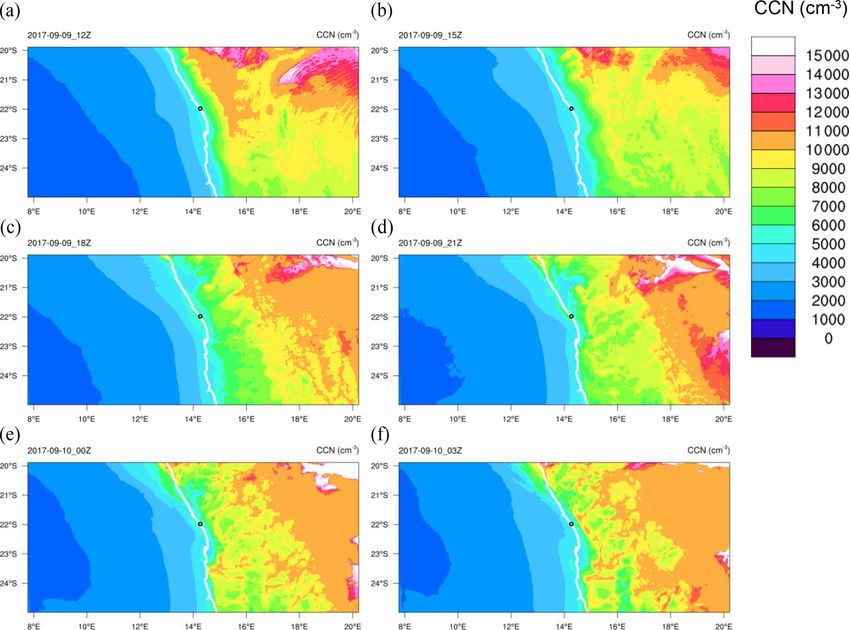
10224                                        M. J. Weston et al.: Sensitivity analysis of an aerosol-aware microphysics scheme

Figure 1. (a) WRF model domains and (b) insert showing the Henties Bay site (star) and inland point (circle) from the model which is used
during the evaluation of the simulations.

2006). The Kain–Fritsch cumulus physics was activated in                 The median volume diameter (MVD) is calculated as fol-
domain 1 but deactivated in domain 2 and 3 (Kain, 2004).               lows:
This allows for subgrid-scale precipitation in the coarse res-
                                                                                 3.672 + µ
olution parent domain, allowing for realistic water balance            MVD =               .                                         (4)
when applying one-way nesting.                                                       λ
                                                                          Fog was diagnosed when liquid water content was present
2.2.1    Fog microphysics                                              in the lowest model level. This is a reasonable assumption
                                                                       for simulations with a suitably high resolution (i.e. observed
The grid-scale cloud microphysics bulk scheme by Thomp-
                                                                       fog feature is larger than model grid cell) and a sophisticated
son and Eidhammer (2014) assumes a gamma distribution of
                                                                       microphysics scheme (Zhou et al., 2012).
cloud DSD for droplet diameters, D, comprised between 1
to 100 µm. It is worth noting that the scheme accounts for
the conversion of cloud droplets to rain droplets, which are           2.2.2   Configuration of the aerosol-aware sensitivity
treated separately, and the rain DSD spans a wider range in                    study
diameter. The number concentration per cloud droplet diam-
                                                                       The Thompson aerosol-aware microphysics scheme
eter, N(D) is calculated as follows:
                                                                       (Thompson and Eidhammer, 2014; hereafter T14) was
             Nt                                                        activated in all three domains to represent grid-scale cloud
N (D) =             λµ+1 D µ e−λD ,                           (1)
          0 (µ + 1)                                                    microphysics. This novel scheme accounts for the initial
                                                                       number concentration, mean radius, and hygroscopicity
where Nt is the total cloud droplet number concentration               (kappa) of CCN and CCN activation to cloud (and other
(cm−3 ), 0 is the gamma function, µ is the shape parame-               hydrometeor) droplets, which ultimately determine the
ter, and λ is the slope. It is a double moment scheme, mean-           maximum number of cloud droplets. Although the default
ing that cloud droplet mass and number concentration (Nt )             settings for these variables are based on observations and the
is calculated from the DSD. The shape and slope parameters             literature, users can refine the values based on their study
can be derived from Nt and liquid water content (LWC) as               area. For example, the initial CCN number concentration
follows:                                                               is set to 300 cm−3 at the lowest model level. This may not
                                                                       be appropriate for a particular study region or event and

            1000
µ = min           + 2, 15 ,                              (2)           can be adjusted accordingly. Furthermore, the option exists
             Nt
                                                                       to replace initial CCN with user-generated 3-D data fields
where Nt is in cubic centimetres (cm−3 ).                              of CCN as input. An example is provided with the model
                                                                       based on a 7-year climatology of aerosols produced by the
                                 1
   π    0 (4 + µ)            Nt      3                                 NASA GEOS (Goddard Earth Observing System)-4 model
λ=   ρw                                  ,                    (3)      (Colarco et al., 2010). A key approach of this scheme is the
   6    0 (1 + µ)           LWC
                                                                       conversion of hygroscopic CCN, sometimes referred to as
where ρw = 1000 kg m−3 is water density, and LWC is in                 water-friendly aerosols, to cloud droplets. This is what is
kilograms per cubic centimetre (kg cm−3 ).                             referred to as CCN activation in this document, which can

Atmos. Chem. Phys., 22, 10221–10245, 2022                                               https://doi.org/10.5194/acp-22-10221-2022
M. J. Weston et al.: Sensitivity analysis of an aerosol-aware microphysics scheme                                           10225

be thought of as the ratio of cloud droplets to hygroscopic        could reach up to 500 cm−3 near the surface (Formenti
CCN. CCN activation is based on parcel method simulations          et al., 2019). Thus, the initial CCN number concentration
by Eidhammer et al. (2009). These simulations were used            near the surface was increase from 300 to 500 cm−3 (here-
to create a look-up table (available within WRF) that varies       after CCN_500), while the free troposphere was kept at
the CCN activation to cloud droplets as a function of CCN          50 cm−3 . CCN_500 has the same vertical profile treatment
number concentration, updraft speed, ambient temperature,          as CCN_300. Initial concentrations over land and the ocean
CCN mean radius diameter, and kappa (hygroscopicity)               were the same, as in CCN_300. In another scenario, the mean
values (Fig. 2). It is important to keep in mind that CCN          radius of the CCN was decreased from 0.04 to 0.02 µm as
activation in the scheme assigns a minimum updraft speed           part of a sensitivity analysis (CCN_300_r0.02 hereafter). All
of 1 cm s−1 when air is saturated. This allows for droplet         other settings were identical to CCN_300. In the final sce-
activation under saturated conditions via the look-up table,       nario, the minimum updraft speed was increased from 0.01
even when the simulated updraft is negative. An additional         to 0.1 m s−1 (CCN_300_w0.1). This motivation for this sce-
novelty of this scheme is that it allows feedback of CCN and       nario was to push the model to a higher CCN activation and
cloud droplets to the radiation schemes in shortwave and           see how this effects the size distribution results. For the last
longwave, which was activated in the model simulations.            scenario, the minimum updraft speed was only assigned in
   Model scenarios were based on configuration of the mi-          the three lowest vertical levels in the model and should not
crophysics, where the default CCN radius is 0.04 µm and            cause erroneous cloud at higher model levels.
the kappa is 0.4 (Fig. 3). Scenario 1 used the default initial        Comparative statistics of model and observed cloud
CCN values of 300 cm−3 near the surface and 50 cm−3 in the         droplet count, LWC, and MVD are presented in the results
free troposphere (hereafter CCN_300). The scheme applies a         section. The model grid point that is closest to the site lo-
vertical profile to CCN concentration, allowing concentra-         cation is extracted for comparison with the observations. A
tions to decrease exponentially from the surface to the free       second model grid point, hereafter referred to as “inland”,
troposphere (WRF Users Page, 2020; Fonseca et al., 2021).          is extracted about 13 km inland when travelling perpendicu-
In summary, the scheme assigns the highest CCN concen-             larly to the coast to demonstrate the dynamics and gradients
tration near the surface and follows an exponential decrease       in the model (Fig. 1b).
through the boundary layer to the minimum bound (50 cm−3
in our case), which is then assigned to the lower free tro-
posphere. The depth of the boundary layer is made to vary          2.3     Observations
for different terrain heights, ranging to about 1000 m at sea      2.3.1    Meteorology and microphysics
level to less than 100 m where terrain is greater than 2500 m.
The thinner boundary layer at increased terrain height would       The AEROCLO-sA ground-based field campaign was con-
have a steeper drop-off in CCN concentration with height and       ducted from 23 August to 12 September 2017 at the Uni-
subsequent dilution during daytime mixing. In CCN_300,             versity of Namibia campus in Henties Bay (−22.09495◦ S,
the initial CCN concentration over land and ocean is the           14.2591◦ E; Formenti et al., 2019). The campus is located on
same. Thompson and Eidhammer (2014) proposed a differ-             the coastline (elevation 20 m a.s.l.) and at the mouth of the
ent initial CCN concentration for land (300 cm−3 ) and ocean       non-perennial Omaruru River.
(100 cm−3 ) based on observations, as ocean air is generally          Measurements pertinent to this study include the mete-
cleaner and contains fewer CCN than continental air (Sein-         orological measurements of temperature (2 m), relative hu-
feld and Pandis, 2016). We implemented this proposal for           midity (2 m), wind speed (10 m), and wind direction (10 m)
scenario 2 (hereafter CCN_300_landsea). The same treat-            from a Cimel Electronique compact weather station, part
ment is applied to the vertical profile of CCN concentra-          of the PortablE Gas and Aerosol Sampling UnitS (PEGA-
tion as CCN_300. Scenario 3 is the default model setting           SUS) mobile platform (Formenti, 2020b). Meteorological
using the 3-D climatology CCN modified from Colarco et             data were supplemented with atmospheric pressure from the
al. (2010; hereafter CCN_C10). As this is a 3-D data set, no       control WRF model simulation described later on. This al-
idealised vertical profile is applied at initialisation. Simula-   lowed further variables to be derived, like the water vapour
tions were run from 7 to 10 September 2017 to coincide with        mixing ratio and air density. Radiosonde measured atmo-
the best data from the fog monitor 100 (FM-100) instrument.        spheric profiles of pressure, temperature, relative humid-
Recall that simulations are initialised at 06:00 UTC and were      ity, wind speed, and wind direction (Formenti, 2020a). Ra-
run for 48 h. The first 6 h are discarded as model spin-up (i.e.   diosonde were launched form two locations, with one being
day 0 during 06:00–11:00 UTC). The next 24 h in the model          at the study site and the other being at Jakkalsputz, about
are used to assess the next-day fog (i.e. day 0 at 12:00 to        12 km south along the coast of the study site. Visibility mea-
day 1 at 11:00 UTC).                                               surements were available from a transmissometer with data
   A sensitivity study to CCN activation was carried out           being recorded every 5 s. The transmissometer is a bistatic
through permutations to the CCN and minimum updraft                system, set up with the emitter and receiver 8.0 m apart and
speed. Initial results from the study site showed that CCN         approximately a metre off the ground. The instrument’s ana-

https://doi.org/10.5194/acp-22-10221-2022                                       Atmos. Chem. Phys., 22, 10221–10245, 2022
10226                                       M. J. Weston et al.: Sensitivity analysis of an aerosol-aware microphysics scheme

Figure 2. CCN activation look-up table. Activated fraction in response to (a) CCN concentration, (b) updraft speed, (c) CCN radius, (d)
ambient temperature, and (e) kappa (hygroscopicity). For each plot, the remaining four variables are kept constant as follows: CCN is
316 cm−3 , updraft is 0.316 m s−1 , radius is 0.04 µm, temperature is 283.15 K, and kappa is 0.4.

Table 1. WRF model scenarios summary. Updraft refers to minimum updraft speed.

                                 Scenario              CCN                     Kappa    Radius   Updraft
                                                       (cm−3 )                           (µm)    (m s−1 )
                             1   CCN_300               300                       0.4      0.04       0.01
                             2   CCN_300_landsea       300/100                   0.4      0.04       0.01
                             3   CCN_C10               Colarco et al. (2010)     0.4      0.04       0.01
                             4   CCN_500               500                       0.4      0.04       0.01
                             5   CCN_300_r0.02         300                       0.4      0.02       0.01
                             6   CCN_300_w0.1          300                       0.4      0.04        0.1

logue voltage output response to optical depth (OD) was cal-          The particle is assumed to be spherical and made of water
ibrated using a series of stacked neutral density filters and         with a known refractive index. Droplets in the size range 2–
found to be linear. This voltage was recorded on a Camp-              50 µm can be counted with bin sizes between 2 and 3 µm. The
bell Scientific CR1000 data logger. From the OD, we cal-              instrument was calibrated with glass beads of known diame-
culate the extinction coefficient and, hence, visibility using        ter and refractive index. The LWC is calculated based on the
Koschmieder’s law. Although this is known to have draw-               assumption that each droplet is spherical. Data were recorded
backs (Lee and Shang, 2016; Nebuloni, 2005), we use the               every second and later aggregated to 1 min averages.
calculated visibility in a qualitative sense in this study.              A cloud condensation nucleus (CCN) counter (mini-
   Cloud droplet measurements were conducted with a fog               CCNC) was deployed at the site. The supersaturation during
monitor 100 (FM-100) providing droplet number concentra-              data capture was set to scanning mode, meaning that super-
tion, size distribution, and liquid water content for particle        saturation varied between 0.1 % and 0.7 %. The CCNC was
sizes with optical equivalent diameter of 1 to 50 µm. This in-        calibrated prior to the campaign using ammonium sulfate to
strument is a forward-scattering spectrometer probe, where            determine the relationship between the temperature gradient
the droplet size is calculated based on scattered light from          along the column and the effective supersaturation. A wide
a laser and employing the Mie theory (Spiegel et al., 2012).          wind-oriented intake facilitated airflow into the instrument

Atmos. Chem. Phys., 22, 10221–10245, 2022                                              https://doi.org/10.5194/acp-22-10221-2022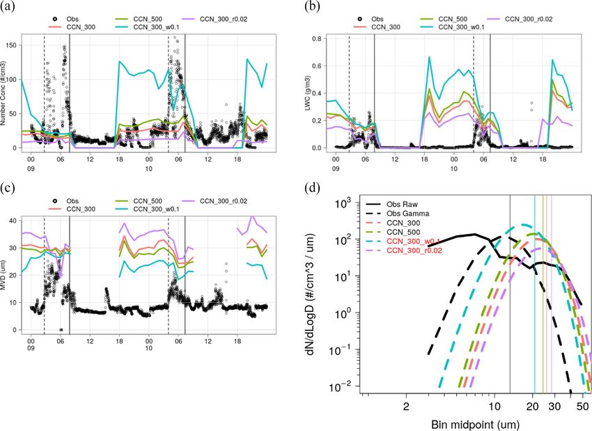
M. J. Weston et al.: Sensitivity analysis of an aerosol-aware microphysics scheme                                          10227

and total CCN was recorded at a high frequency (every sec-         3     Results and discussion
ond).
                                                                   3.1     Case study description
2.3.2   Activated CCN                                              There were two fog events observed on consecutive days on
                                                                   9 and 10 September 2017 (hereafter case 1 and case 2, re-
Activated CCN, the percentage of hygroscopic CCN that are
                                                                   spectively) during the AEROCLO-sA campaign at Henties
present as cloud droplets as described in the model micro-
                                                                   Bay (Fig. 3). Visibility dropped below 1 km from about 03:00
physics section, can be estimated as measurements of cloud
                                                                   to 07:00 UTC during case 1. The wind direction was pre-
droplets (from FM-100) and CCN (from mini-CCNC) are co-
                                                                   dominantly northwesterly and veering to northeasterly dur-
located. This definition is maintained in the processing of the
                                                                   ing these days, which is in contrast to the dominant wind
observations to allow for consistency in comparing the model
                                                                   direction of southwesterly during the full campaign dates.
microphysics scheme with observations. Data overlap from
                                                                   Wind speed was 2 m s−1 or less during the events. Water
these instruments coincided with a fog event on 9 Septem-
                                                                   vapour mixing ratio ranged between 8 and 10 g kg−1 dur-
ber 2017, which was used to estimate the activated CCN at
                                                                   ing the fog events but was more than 10 g kg−1 during the
the site. The CCN counter cycled through supersaturation
                                                                   day. The observed relative humidity remained over 90 %
from 0.1 % to 0.7 % to account for varying aerosol sizes.
                                                                   throughout the case study period. A temperature inversion
For our purposes, CCN data were subset to supersaturation
                                                                   with a strength of about 10 ◦ C was present on both morn-
range from 0.098 % to 0.151 %. Practically, this means that
                                                                   ings below 1000 m a.s.l. Satellite images for case 1 indicate
CCN data are available at about 3 min intervals due to the
                                                                   an isolated cloud over the study site from 00:00 UTC, and
supersaturation cycle of the instrument. The 1 s data were
                                                                   by 03:00 UTC, the fog patch is elongated along the coast-
then averaged to 1 min for both the CCN and FM-100 and
                                                                   line (Fig. 4). No cloud is present over the ocean, and this fog
paired according to matching times. CCN concentration is
                                                                   patch is not associated with a stratus deck. For case 2, visi-
expected to be underestimated during wet conditions due to
                                                                   bility dropped below 1 km from 04:00 to 07:00 UTC. Satel-
the design of the inlet on the instrument. To overcome this,
                                                                   lite images indicate that cloud was present over the site from
we use the CCN concentration in the period prior to fog in
                                                                   16:00 UTC the day before and was associated with stratus
the activated CCN calculation. A period of 1 h of observa-
                                                                   over the ocean (Fig. 5). This cloud gradually advected over
tions when visibility was 10 km prior to fog formation was
                                                                   the land, and by 21:00 UTC, the visibility had decreased to
used as the CCN sample. This period occurred from 01:00 to
                                                                   2 km. By 03:00 UTC, just before fog onset, the stratus deck
02:05 UTC on 9 September 2017. The average CCN concen-
                                                                   had increased extent over the ocean. After sunrise, the cloud
tration was calculated for this period and used in conjunc-
                                                                   over the land dissipated, while the cloud over the ocean re-
tion with the Nt during fog conditions to calculate activated
                                                                   mained through the day and into the following night.
CCN as Nt / CCN (cm−3 ). Lastly, the data were filtered for
conditions where Vis < = 1 km (based on the World Meteo-
rological Organization, 2008, definition) and Nt > 25 cm−3 ,       3.2     Activated CCN
where the visibility threshold meant that fog conditions were
                                                                   The activated CCN calculated from the observations, as de-
represented, and the Nt threshold was estimated as being rep-
                                                                   scribed in Sect. 2.3.2, ranged from 0.058 to 1 (i.e. 5.8 % to
resentative of a baseline in the fog monitor.
                                                                   100 %), where 1 is the theoretical maximum (Fig. 6). The
                                                                   median (mean) was 0.55 (0.56), and the standard deviation
2.3.3   Satellite                                                  was 0.24. When the fog was most dense, represented by the
                                                                   highest Nt values between 06:30 and 07:15 UTC, the acti-
The spatial evolution of the cloud and fog is presented
                                                                   vated CCN reached over 80 %. Values of CCN activation of
using the Spinning Enhanced Visible and Infrared Imager
                                                                   0.8 at 0.1 % supersaturation are possible and have been ob-
(SEVIRI) from Meteosat Second Generation 3 (MSG-3;
                                                                   served (Che et al., 2016). When considering the CCN acti-
Schmetz et al., 2002). MSG3, also known as the Meteosat
                                                                   vation look-up table from WRF (Fig. 2), an updraft speed
10 satellite, is in a geostationary orbit over 9.5◦ E. Nighttime
                                                                   of 0.1 m s−1 corresponds to CCN activation just below 0.3.
scenes are false colour composite images using the night mi-
                                                                   Therefore, assigning a minimum updraft speed of 0.1 m s−1
crophysical product from EUMETSAT (European Organiza-
                                                                   can be a reasonable assumption, as it falls within the median
tion for the Exploitation of Meteorological Satellites; Eumet-
                                                                   of activation at the site 0.56.
sat, 2009). This product is a red–green–blue (RGB) compos-
ite, where the red channel is the difference between 12.0 and
10.8 µm channels (linear stretch −4 to 2 K), green is the dif-     3.3     Analysis of simulations
ference between 10.8 and 3.9 µm channels (linear stretch 0 to      3.3.1    Evaluation of simulated meteorology
10 K), and blue is the 10.8 µm channel (linear stretch 243 to
293 K). Daytime scenes are an RGB of the visible channels          The observed daily temperature range at the study site is nar-
(R is VIS 06; G is VIS 0.8; B is IR 1.6).                          row and did not exceed 5 ◦ C, which is a clear indication of

https://doi.org/10.5194/acp-22-10221-2022                                        Atmos. Chem. Phys., 22, 10221–10245, 2022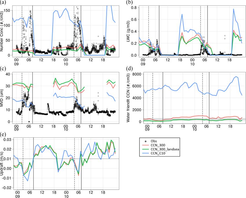
10228                                       M. J. Weston et al.: Sensitivity analysis of an aerosol-aware microphysics scheme

                                                                      the observed inversion (Fig. 8). Subsequently, the moisture
                                                                      and associated relative humidity was over 80 % near the sur-
                                                                      face and decreased rapidly from the base of the inversion to
                                                                      10 % at around 600 m. It is worth noting that the observed
                                                                      relative humidity at the surface was below 100 % and peaked
                                                                      near 100 % at about 250 m, while the model was at 100 %
                                                                      at the corresponding heights. For case 2, the base of the ob-
                                                                      served temperature inversion was higher at about 800 m and
                                                                      coincided with the peak relative humidity of 100 % (Fig. 9).
                                                                      The model inversion height was also higher than case 1
                                                                      model results but was still below 500 m. The reason for the
                                                                      higher inversion level during case 2 is not clear. This could be
                                                                      attributed to the difference in timing of the sonde (1 h later)
                                                                      or that the fog event is optically thick and has a major ef-
                                                                      fect on the radiation (as in Price, 2011; Boutle et al., 2018).
                                                                      Nevertheless, the model is capturing a low level surface in-
                                                                      version trapping the moisture below this inversion, as in the
Figure 3. Meteorological variables from the Cimel Electronique
                                                                      observations.
compact weather station at the site during the two fog events on
9 and 10 September 2017. The variables are temperature (T in          3.3.2   Spatial distributions of CCN and cloud droplet
degrees Celsius), water vapour mixing ratio (q), relative humidity            concentration
(RH), wind direction (wd), wind speed (ws), and visibility (Vis)
from the transmissometer. Vertical black dashed (solid) lines indi-   The initial CCN concentration for CCN_300 is similar over
cate fog start (end) times. The x axis shows hours in UTC (site is    land and ocean (Fig. 10a). However, over time, the concen-
UTC+2) and the day of the month in September.                         tration over the ocean is relatively higher than over the land,
                                                                      as is evident in the mean concentration in Fig. 10b. This is
                                                                      counter-intuitive, as observed CCN concentrations are typi-
the maritime influence on modulating temperature (Fig. 7a).           cally lower over the ocean than the land (Seinfeld and Pan-
The modelled diurnal temperature range is larger and more             dis, 2016). The relative decrease in concentration over the
representative of a terrestrial site, with the maximum tem-           land is most likely due to the treatment of the vertical dis-
perature being 4–5 ◦ C warmer and the minimum between 1–              tribution of CCN in the scheme, where CCN concentrations
5 ◦ C colder than observed. The combination of model hori-            have a steeper decrease with height when terrain height is
zontal resolution and physics may be limited to resolve the           above 1000 m. This allows for the dilution of the surface
exact location of the land–sea interface occurring at the sam-        CCN concentration during vertical mixing of the atmosphere.
pling site, which is within 200 m of the sea shore. Conse-            Furthermore, the boundary conditions for scenario CCN_300
quently, the cold bias may trigger early saturation, as sug-          had relatively lower concentrations of CCN than the ambient
gested by the relative humidity time series in Fig. 7e. The           CCN in the domain. This explains the lower CCN concen-
water vapour mixing ratio is underestimated by 2 to 4 g kg−1          trations over the southern part of the ocean in the domain as
during the nighttime, but this is not dry enough to prevent           clean air was advected from the boundary conditions.
saturation. Simulated wind speed is within 1 m s−1 for most              The initial CCN concentration for scenario
of the simulation and, more importantly, during the observed          CCN_300_landsea shows a clear contrast, with lower
fog periods (Fig. 7b). However, the maximum bias is 2 m s−1           concentration over the ocean than the land (Fig. 10c). The
(negative) during the night of 8 September, and the model             lower concentration over the ocean counteracts the accu-
underestimated the daytime wind speed on 9 September by               mulation of CCN over time, as seen in CCN_300, resulting
approximately 2 m s−1 . The observed wind direction shifts            in a more balanced mean CCN concentration between land
from southwesterly on 8 September to northerly during the             and ocean (Fig. 10d). Scenario CCN_C10 has an order of
case studies. The simulation captures this progression, al-           magnitude higher for the concentration of CCN (Fig. 10e
though the model shifts back to southerly during the day of           and f) and does exhibit higher concentrations over land
9 September (coinciding with the underestimated maximum               than the ocean. This contrast is maintained though out the
wind speed) before veering back to northerly.                         simulation as the terrain-dependent vertical profile described
   The modelled profiles of temperature and relative humid-           earlier is not applied to these CCN. Furthermore, as the CCN
ity displayed the low level inversion and moisture, as seen           are a subset of a larger data set, the boundary conditions
in the observed profiles. For case 1, the model captured the          include similarly higher concentrations of CCN, and clean
near-surface temperature inversion at about the same height           air is not advected into the domain.
(base of inversion is at ∼ 250 m) and strength (∼ 10 ◦ C) as

Atmos. Chem. Phys., 22, 10221–10245, 2022                                             https://doi.org/10.5194/acp-22-10221-2022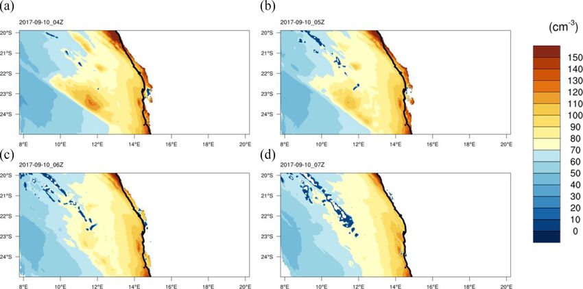
M. J. Weston et al.: Sensitivity analysis of an aerosol-aware microphysics scheme                                             10229

Figure 4. SEVIRI images of night microphysical RGB product (a–e) and day visible channels (f–j) for the fog event on 9 September 2017.
The yellow open circle is the study site. The site is UTC+2. The extent matches the WRF model 3 km domain, which extends 1386 km
(east–west) by 720 km (north–south).

   The evolution of CCN concentration for CCN_300 dur-               onto the low-lying Namib desert is also evident. At Henties
ing case 2 is shown in Fig. 11. It clearly shows that, by            Bay, the wind direction is southwesterly (200◦ ) from 12:00
12:00 UTC (forecast hour 7), the concentration over the              to 18:00 UTC and veers to northwesterly (300◦ ) from about
ocean is higher (500–600 cm−3 ) than over the land in the            19:00 to 06:00 UTC. This northwesterly flow allows for the
lowest model level. The clean air from the boundary con-             low level transport of the accumulated CCN back along the
ditions is evident in the south and continues to propagate           coastline.
through the domain throughout the forecast. Ahead of this               The fog onset, represented by cloud droplet concentration,
advection, concentration increases as CCN are transported            is shown in Fig. 12, where droplet concentration reached up
from the south and accumulate. An onshore flow of CCN                to 50 cm−3 . Over land, fog starts to form along the coast first

https://doi.org/10.5194/acp-22-10221-2022                                          Atmos. Chem. Phys., 22, 10221–10245, 2022
10230                                       M. J. Weston et al.: Sensitivity analysis of an aerosol-aware microphysics scheme

Figure 5. SEVIRI images of night microphysical RGB product (b–e) and day visible channels (a, f, g) for the fog event on 10 Septem-
ber 2017. The yellow open circle is the study site. The site is UTC+2. The extent matches the WRF model 3 km domain, which extends
1386 km (east–west) by 720 km (north–south).

Figure 6. Time series of (a) CCN (cm−3 ), (b) Nt (cm−3 ), (c) activated CCN (proportion), and (d) visibility during the fog event on
9 September 2017. Red dots indicate data points used to calculate activated CCN. Blue dots are not used to calculate activated CCN and are
shown for context. Times are in UTC (site is UTC+2).

Atmos. Chem. Phys., 22, 10221–10245, 2022                                               https://doi.org/10.5194/acp-22-10221-2022
M. J. Weston et al.: Sensitivity analysis of an aerosol-aware microphysics scheme                                                10231

Figure 7. Time series of model and observed meteorological variables at Henties Bay for (a) temperature, (b) wind speed, (c) water vapour
mixing ratio, (d) wind direction, and (e) relative humidity. Times are in UTC (site is UTC+2).

and then extends further inland, signifying that the simulated          mixing of marine CCN in the Namib desert is still evident,
fog is due to advection and not to radiation. Radiation fog             meaning that the study site is influenced by the marine CCN
would be expected to form inland first, or simultaneously               during these simulations.
with coastal fog, as the radiative cooling should be stronger              Fog onset over the land is similar to CCN_300, as this is
inland (e.g. Weston and Temimi, 2020). The fog reached                  controlled by the ambient conditions. However, cloud droplet
maximum inland extent at 04:00 UTC (Fig. 13a) before dis-               concentration is 2 to 3 times higher in general compared to
sipating inland by 07:00 UTC (Fig. 13d). Cloud droplets are             CCN_300, reaching up to 150 cm−3 (Fig. 15). Even though
present over the ocean from 21:00 to 07:00 UTC. The spa-                the percentage of droplet activation decreases as CCN con-
tial distribution of CCN and cloud droplet concentration for            centration increases (Fig. 2a), the initial CCN is significantly
CCN_300_landsea were similar to CCN_300, although the                   high enough to activate more cloud droplets than CCN_300.
concentrations were generally lower.                                    As in CCN_300, cloud droplets are present over the ocean
   The evolution of CCN concentration for CCN_C10 dur-                  from 21:00 to 07:00 UTC. The maximum fog extent over the
ing case 2 is shown in Fig. 14. What is notable is the lack of          land (Fig. 16) is a good match to the satellite data (Fig. 5).
clean air advection from the boundary conditions, the relative             In general, the first three scenarios did well in capturing
contrast in concentration between land and ocean is main-               the fog extent over the land. They show the cloud forming at
tained throughout, and there is generally less variation over           the coast first before moving inland, suggesting that the dy-
time compared to CCN_300. However, the onshore flow and                 namics of the formation are captured in the model. Over the

https://doi.org/10.5194/acp-22-10221-2022                                             Atmos. Chem. Phys., 22, 10221–10245, 2022
10232 M. J. Weston et al.: Sensitivity analysis of an aerosol-aware microphysics scheme
ocean in terms of CCN and cloud droplet concentrations. Ad-
ditionally, the semi-permanent cloud deck in the simulations
impinges onto the adjacent land, mainly due to the onshore
flow. Similar patterns of excess frequency of cloud cover (by
30 % to 50 %) over the ocean were reported for a regional cli-
mate model simulation over Namibia (Haensler et al., 2011).
They demonstrate the same high contrast between ocean and
land and highlight that the study sites at the coast fall within
a transition zone in the model. The study site is located at the
interface between these two contrasting conditions and falls
within the impingement zone of the simulations. This must
be kept in consideration when comparing the model micro-
physics to the observations from the site, which will be dis-
cussed in the following section.
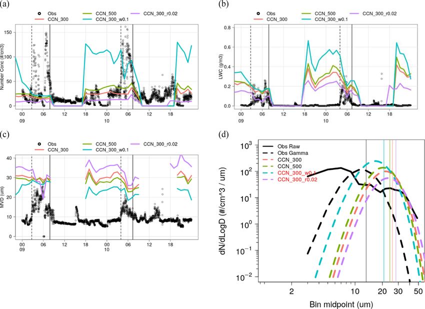
3.3.3 Comparison of simulated and observed fog
microphysics
Figure 8. Radiosonde profiles of (a) temperature and (b) relative
humidity from Jakkalsputz on 9 September 2017. The sonde was The observed microphysics during case 1 showed cloud
launched at 07:50 UTC, and the model is from 08:00 UTC. The site droplet number concentrations of up to 150 cm−3 (mean of
is UTC+2. 42 cm−3 ), maximum LWC around 0.25 g m−3 , and MVD up
to 27 µm (Fig. 17a–c). Case 2 demonstrated a higher mean
number concentration of 79 cm−3 , LWC peaked at 0.3 g m−3 ,
and MVD was lower up to 21 µm.
During case 1, the cloud droplet number concentration was
below 25 cm−3 for CCN_300, approximately 6 times less
than the observations. However, the LWC was comparable
to the observations at about 0.2 g m−3 . This means that the
LWC is distributed among fewer droplets than the observa-
tions and that the DSD will shift towards larger droplet di-
ameters, which is evident in the MVD around 30 µm. The
model exhibited larger number concentrations during case 2,
which appears to be associated with higher CCN concentra-
tions (Fig. 17d). This, in turn, results in marginally increased
LWC and an associated decrease in the MVD. As expected,
CCN_300_landsea was similar to CCN_300 but with lower
cloud droplet concentrations due to lower CCN concentra-
tions. The CCN concentrations were within the observed
mean CCN concentration, which could be a good starting
point for sensitivity tests on percentage droplet activation for
Figure 9. Radiosonde profiles of (a) temperature and (b) relative the future. The modelled updraft speed at the site was low,
humidity from Jakkalsputz on 10 September 2017. The sonde was i.e. below 0.02 m s−1 prior to fog formation and either neg-
launched at 09:10 UTC, and the model is from 09:00 UTC. ative or below 0.01 m s−1 during fog (Fig. 17e). This means
that the applied updraft speed is the minimum updraft speed
from Table 1 when the microphysics is activated.
ocean, cloud droplet activation is overactive, as a cloud deck The scenario CCN_C10 has around 10 times higher initial
is present from 21:00 UTC (Figs. 12 and 15a). At night, the concentrations of CCN throughout the simulation. This re-
air over the ocean is saturated (not shown), which we assume sulted in cloud droplet concentrations around 125 cm−3 dur-
is from either a cold bias or positive bias in the water vapour ing case 1 and case 2, which was comparable with the ob-
mixing ratio. Saturation is the first condition that must be met servations. Case 2 was marginally lower than case 1 in this
for droplet activation, and it is assumed this is causing a per- simulation, as the CCN were lower. The maximum LWC dur-
sistent cloud deck over the ocean. The cloud deck was also ing case 1 was about the same as the observed at 0.25 g m−3
present in case 1 simulations, while the satellite shows no and just over 0.3 g m−3 during case 2. As the cloud droplet
cloud is present over the ocean. It has been demonstrated now number concentration and LWC are comparable to the obser-
that, in all scenarios, there is a contrast between the land and vations, the MVD was much closer, with a maximum around
Atmos. Chem. Phys., 22, 10221–10245, 2022 https://doi.org/10.5194/acp-22-10221-2022M. J. Weston et al.: Sensitivity analysis of an aerosol-aware microphysics scheme 10233 Figure 10. Initial and mean water-friendly CCN concentration (cm−3 ) for scenarios (a, b) CCN_300, (c, d) CCN_300_landsea, and (e, f) CCN_C10. Note the different scale in panel (c). The black dot is Henties Bay. 20 µm for both cases. This scenario demonstrated the best (Fig. 17a). From this point, droplets persist or are activated performance in terms of cloud microphysics at the site, which whenever saturation is met until the case 2 event. The po- is interesting as the initial CCN values appear to be largely tential drawback of using the updraft velocity to define drop overestimated. The reported mean of CCN at the site ranged activation for fog formation has been discussed previously from 230–550 cm−3 (Formenti et al., 2019), while the mod- (Boutle et al., 2018; Poku et al., 2019). The argument is that elled CCN was above 4000 cm−3 throughout the simulation. fog often forms under stable conditions when no updraft is As presented in Sect. 3.2, the observed CCN activation can present and that activation is instead due to the cooling of the be between 20 % and 80 % during fog events, while the mod- air. In addition, the threshold updraft speed is often higher elled activation is much lower, at around 10 %. To understand than the 0.01 m s−1 used in the T14 scheme, which effec- this further, we need to discuss CCN activation in the model tively results in a higher supersaturation and excess droplet scenarios. activation than would be expected for a fog event (Boutle et CCN activation is most sensitive to CCN concentration al., 2018; Poku et al., 2019). Reported activation fractions and then updraft speed. For each scenario, the CCN con- of CCN in fog are around 20 % but reach up to 40 % (Ma- centration is always present and does not vary greatly. Keep zoyer et al., 2019). To some extent, the implementation of in mind that the mean radius and kappa values are constant a relatively low updraft speed in the look-up table mitigates throughout. against excess droplets forming in the T14 scheme. Activa- The updraft speed during both cases was negative, mean- tion at speeds less than 0.03 m s−1 are around 10 % or less. ing that the minimum updraft of 1 cm s−1 is applied. If we Thompson and Eidhammer (2014) acknowledge the use of consider case 2, we can see that the saturation is met at updraft speed as a potential limitation in the scheme in terms 18:00 UTC, and droplets are formed prior to the fog event of fog formation. Their proposed workaround is to include https://doi.org/10.5194/acp-22-10221-2022 Atmos. Chem. Phys., 22, 10221–10245, 2022
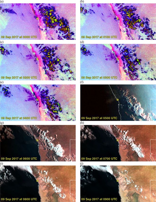
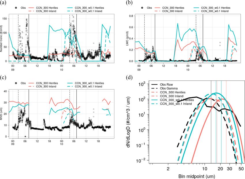
10234                                    M. J. Weston et al.: Sensitivity analysis of an aerosol-aware microphysics scheme

Figure 11. Evolution of water-friendly CCN concentration (cm−3 ) for the event on 10 September 2017 for scenario CCN_300. The black
dot is Henties Bay. Time is in UTC (site is UTC+2).

cooling tendency as proxy for updraft speed and then as-            larger droplets and spectrum widening in a maturing cloud
signing a speed that will activate the appropriate number of        (e.g. Egli et al., 2015; Mazoyer et al., 2019). From the model
droplets. This may come with a new set of problems in terms         scenarios, CNN_C10 demonstrates the best match with the
of early activation, but this remains to be seen.                   observations (Fig. 19), with the best performance in case 2.
   The observed DSD needs to be transformed to a gamma              For the scenarios where initial CCN is constant, the distribu-
distribution in order to compare it to the model. This is pos-      tion shifts to larger droplet sizes.
sible as the only inputs to the shape and slope parameters are         The results of the sensitivity analysis are discussed be-
the number concentration and LWC (Eqs. 2 and 3). The mean           low. The influence of number concentration on LWC and
number concentration and LWC for each case was used, and            MVD is further highlighted by the CNN_500 scenario. For
the transformation of the observed (Obs_raw) and gamma              all times, this scenario has higher cloud droplet concentra-
distribution (Obs_gamma) can been seen in Fig. 18. While            tions that CCN_300 (Fig. 20a). This results in overall higher
the observations show signs of a trimodal distribution with         LWC and lower MVD (Fig. 20b and c). The inverse is shown
peaks around 7, 16, and 30 µm, the gamma distribution has           with scenario CNN_300_r0.02. In this scenario, the radius
one peak at around 11 µm. The three modes in the observed           of the CCN was halved, which results in a lower num-
distribution could be representative of the various CCN pop-        ber of activated droplets, according Kohler theory (Fig. 2b).
ulations, where larger salt particles with higher kappa val-        Similar sensitivity analyses have been reported by Poku et
ues could represent the largest mode, while the smaller sul-        al. (2019) and Stolaki et al. (2015). The most interesting re-
fates represent the smaller modes. Droplet growth by col-           sults comes from scenario CCN_300_w0.1, which demon-
lision and coalescence can be another explanation for the           strated the closest match to the observed number concentra-

Atmos. Chem. Phys., 22, 10221–10245, 2022                                           https://doi.org/10.5194/acp-22-10221-2022
M. J. Weston et al.: Sensitivity analysis of an aerosol-aware microphysics scheme                                             10235

Figure 12. Cloud droplet concentration (cm−3 ) onset for the event on 10 September 2017 for scenario CCN_300. The black dot is Henties
Bay. Time is in UTC (site is UTC+2).

Figure 13. Cloud droplet concentration (cm−3 ) during maximum extent and highest concentration for the event on 10 September 2017 for
scenario CCN_300. Maximum extent was at (a) 04:00 UTC and maximum concentration at Henties Bay was at (d) 07:00 UTC. The black
dot is Henties Bay.

https://doi.org/10.5194/acp-22-10221-2022                                          Atmos. Chem. Phys., 22, 10221–10245, 2022
10236                                     M. J. Weston et al.: Sensitivity analysis of an aerosol-aware microphysics scheme

Figure 14. Evolution of CCN concentration for the event on 10 September 2017 for scenario CCN_C10. The black dot is Henties Bay.

tion, LWC, and MVD. The logic behind this scenario was to           Therefore, the use of a minimum updraft speed of 0.1 m s−1
increase the number of activated droplets by increasing the         does not have a physical basis in our simulation and is used
minimum updraft speed from 0.01 to 0.1 m s−1 , which should         only as part of the sensitivity analysis. It is also clear that if
allow around 30 % activation. Here we have a scenario in            we use a physical basis for the minimum updraft speed, then
which both the CCN and cloud droplet number are in line             the model will not activate enough cloud droplets and that
with the observations. This follows on from the discussion          another physical process must be manifesting the droplet ac-
of using temperature tendency as a proxy for updraft speed,         tivation.
showing that it could work if the nucleation percentage is             In our case, we assume that the observed fog events are due
known and an appropriate updraft speed is assigned. How-            to cloud base lowering (CBL). The satellite images in Figs. 4
ever, in our case, the minimum updraft speed of 0.1 m s−1           and 5 indicate that cloud is present over the site before fog
may relate to an unrealistic cooling rate for this fog event,       is observed in the surface observations (Fig. 3). The surface
which we discuss below.                                             observations indicate that fog starts at 02:43 and 04:00 UTC
   An updraft speed of 0.1 m s−1 equates to a cooling rate          on 9 and 10 September, respectively (Fig. 3). Cloud is visible
of 3.51 K h−1 (2.34 K h−1 ) at the dry (wet) adiabatic lapse        from the satellite from 01:00 UTC on 9 September and even
rate. Our observed cooling rate at 2 m air temperature is be-       16:00 UTC on 9 September prior to the fog on 10 September.
low 1 K h−1 prior to the fog formation (Fig. 3). A cooling          From the literature, cloud base lowering fog events do not
rate of 1 K h−1 equates to an updraft speed between 0.028           show the same cooling rate at the surface as radiation fog,
and 0.04 m s−1 at the dry and wet adiabatic, respectively. The      as the overhead cloud inhibits cooling (e.g. Román-Cascón
modelled updraft speed is below 0.02 m s−1 prior to fog for-        et al., 2019). Furthermore, the influence of the maritime en-
mation and therefore in line with the observed cooling rate.        vironment at the site will dampen cooling from the desert

Atmos. Chem. Phys., 22, 10221–10245, 2022                                            https://doi.org/10.5194/acp-22-10221-2022
M. J. Weston et al.: Sensitivity analysis of an aerosol-aware microphysics scheme                                              10237

Figure 15. Cloud droplet concentration (cm−3 ) onset for the event on 10 September 2017 for scenario CCN_ C10. The black dot is Henties
Bay.

Figure 16. Cloud droplet concentration (cm−3 ) during maximum extent and highest concentration for the event on 10 September 2017 for
scenario CCN_C10. Maximum extent was at (a) 04:00 UTC and maximum concentration at Henties Bay was at (d) 07:00 UTC. The black
dot is Henties Bay.

https://doi.org/10.5194/acp-22-10221-2022                                          Atmos. Chem. Phys., 22, 10221–10245, 2022
10238                                         M. J. Weston et al.: Sensitivity analysis of an aerosol-aware microphysics scheme

Figure 17. Observed and modelled (a) Nt , (b) LWC, and (c) MVD at Henties Bay. The model is hourly, and black dots are 1 min observations.
(d) Modelled concentrations of water-friendly aerosols. (e) Modelled updraft speed in lowest model level with solid black line at minimum
updraft in microphysics scheme. Time is in UTC (site is UTC+2).

Figure 18. (a) Time series of cloud droplet count (Nt ) and visibility. Vertical dashed lines represent sonde release times. The grey horizontal
line at 1 km visibility represents fog conditions. Time is in UTC (site is UTC+2). (b) Droplet size distribution for the two case studies when
visibility was 1 km or less is shown. Colours match with the colours in the time series. Solid lines are the observed distributions. Dashed
lines are the equivalent theoretical gamma distribution applied to the observed data.

Atmos. Chem. Phys., 22, 10221–10245, 2022                                                   https://doi.org/10.5194/acp-22-10221-2022
You can also read