Temporal inventory of glaciers in the Suru sub-basin, western Himalaya: impacts of regional climate variability - ESSD
←
→
Page content transcription
If your browser does not render page correctly, please read the page content below
Earth Syst. Sci. Data, 12, 1245–1265, 2020
https://doi.org/10.5194/essd-12-1245-2020
© Author(s) 2020. This work is distributed under
the Creative Commons Attribution 4.0 License.

          Temporal inventory of glaciers in the Suru sub-basin,
                western Himalaya: impacts of regional
                           climate variability
               Aparna Shukla1,2 , Siddhi Garg1 , Manish Mehta1 , Vinit Kumar1 , and Uma Kant Shukla3
                     1 WadiaInstitute of Himalayan Geology, 33 GMS Road, Dehradun, 248001, India
                                  2 Ministry of Earth Sciences, New Delhi, 110003, India
                       3 Department of Geology, Banaras Hindu University, Varanasi, 221005, India

                            Correspondence: Aparna Shukla (aparna.shukla22@gmail.com)

                                  Received: 13 July 2019 – Discussion started: 19 August 2019
                          Revised: 5 February 2020 – Accepted: 20 April 2020 – Published: 5 June 2020

      Abstract. The importance of updated knowledge about the glacier extent and characteristics in the Himalaya
      cannot be overemphasized. Availability of precise glacier inventories in the latitudinally diverse western Hi-
      malayan region is particularly crucial. In this study we have created an inventory of the Suru sub-basin in the
      western Himalaya for the year 2017 using Landsat Operational Land Imager (OLI) data. Changes in glacier pa-
      rameters have also been monitored from 1971 to 2017 using temporal satellite remote-sensing data and limited
      field observations. Inventory data show that the sub-basin has 252 glaciers covering 11 % of the basin, hav-
      ing an average slope of 25 ± 6◦ (standard deviations have been italicized throughout the text) and dominantly
      north orientation. The average snow line altitude (SLA) of the basin is 5011 ± 54 m a.s.l. with smaller (47 %)
      and cleaner (43 %) glaciers occupying the bulk area. Long-term climate data (1901–2017) show an increase in
      the mean annual temperature (Tmax and Tmin ) of 0.77 ◦ C (0.25 and 1.3 ◦ C) in the sub-basin, driving the overall
      glacier variability in the region. Temporal analysis reveals a glacier shrinkage of ∼ 6 ± 0.02 %, an average re-
      treat rate of 4.3 ± 1.02 m a−1 , debris increase of 62 % and a 22 ± 60 m SLA increase in the past 46 years. This
      confirms their transitional response between the Karakoram and the Greater Himalayan Range (GHR) glaciers.
      Besides, glaciers in the sub-basin occupy two major ranges, the GHR and Ladakh Range (LR), and experience
      local climate variability, with the GHR glaciers exhibiting a warmer and wetter climate as compared to the LR
      glaciers. This variability manifests itself in the varied response of GHR and LR glaciers. While the GHR glaciers
      exhibit an overall rise in SLA (GHR: 49 ± 69 m; LR: decrease of 18 ± 50 m), the LR glaciers have deglaciated
      more (LR: 7 %; GHR: 6 %) with an enhanced accumulation of debris cover (LR: 73 %; GHR: 59 %). Inferences
      from this study reveal prevalence of glacier disintegration and overall degeneration, transition of clean ice to
      partially debris-covered glaciers, local climate variability and non-climatic (topographic and morphometric)-
      factor-induced heterogeneity in glacier response as the major processes operating in this region. The Shukla et
      al. (2019) dataset is accessible at https://doi.org/10.1594/PANGAEA.904131.

Published by Copernicus Publications.
1246                               A. Shukla et al.: Temporal inventory of glaciers in the Suru sub-basin, western Himalaya

1   Introduction                                                   ing behaviour is observed for the Greater Himalayan Range
                                                                   (GHR) glaciers experiencing large-scale degeneration, with
The state of the Himalayan cryosphere has a bearing on mul-        more than 65 % of glaciers retreating between 2000 and 2008
tiple aspects of hydrology, climatology, the environment and       (Scherler et al., 2011). However, there are two views pertain-
sustenance of living organisms at large (Immerzeel et al.,         ing to the glaciers in the Trans-Himalayan range, with one
2010; Miller et al., 2012). Being sensitive to the ongoing         suggesting their intermediate response between the Karako-
climate fluctuations, glaciers keep adjusting themselves, and      ram Himalaya and GHR (Chudley et al., 2017) and the
these adaptations record the changing patterns in the global       other emphasizing their affinity either towards the GHR or
climate (Bolch et al., 2012). Any alteration in the glacier pa-    the Karakoram Himalayan glaciers (Schmidt and Nuesser,
rameters would ultimately affect the hydrology of the region,      2017). Therefore, in order to add more data and build a com-
thereby influencing the downstream communities (Kaser et           plete understanding of the glacier response, particularly in
al., 2010; Pritchard, 2017). Owing to these reasons, quanti-       the western Himalaya, more local-scale studies are neces-
fying the mass loss over different Himalayan regions in the        sary.
past years as well as ascertaining the present status of the          Complete and precise glacier inventories form the basic
cryosphere and how these changes are likely to affect the          prerequisites not only for comprehensive glacier assessment
freshwater accessibility in the region is at the forefront of      but also for various hydrological and climate-modelling-
contemporary cryospheric research (Brun et al., 2017; Sakai        related applications (Vaughan et al., 2013). Information on
and Fujita, 2017). This aptly triggered several regional (Kääb     spatial coverage of glaciers in any region is a much valued
et al., 2012; Gardelle et al., 2013; Brun et al., 2017; Zhou       dataset and holds paramount importance in the future assess-
et al., 2018; Azam et al., 2018; Maurer et al., 2019), local       ment of glaciers. Errors in the glacier outlines may propagate
(Bhushan et al., 2018; Vijay and Braun, 2018) and glacier-         and introduce higher uncertainties in the modelled outputs
specific studies (Dobhal et al., 2013; Bhattacharya et al.,        (Paul et al., 2017). Besides, results from modelling studies
2016; Azam et al., 2016) in the region. These studies at vary-     conducted over the same region but using different sources of
ing scales contribute towards solving the jigsaw puzzle of         glacier boundaries are rendered incomparable, constraining
the Himalayan cryosphere. The regional-scale studies oper-         the evaluation of models and thus their future development.
ate on a small scale for bringing out more comprehensive,          On the other hand, quality, accuracy and precision associated
holistic and synoptic spatio-temporal patterns of glacier re-      with glacier-mapping and outline delineation require dedi-
sponse; the local-scale studies monitor glaciers at the basin or   cated efforts. Several past studies discuss the methods for and
group level and offer more details on heterogenous behaviour       challenges associated with achieving an accurate glacier in-
and plausible reasons thereof. However, the glacier-specific       ventory and resolutions for the same (Paul et al., 2013, 2015,
studies, whether based on field, satellite or integrative infor-   2017). Thorough knowledge of glaciology and committed
mation, are magnified versions of the local-scale studies and      manual endeavour are two vital requirements in this regard.
hold the potential to provide valuable insights into various       Realization of the above facts has resulted in several devoted
morphological, topographic and local climate-induced con-          attempts to prepare detailed glacier inventories at a global
trols on glacier evolution. Despite these efforts, data on the     scale, such as the Randolph Glacier Inventory (RGI), Global
glacier variability and response remain incomplete, knowl-         Land Ice Measurements from Space (GLIMS) and recently
edge of the governing processes is still preliminary and the       the Chinese Glacier Inventory (CGI) and Glacier Area Map-
future-viability pathways of the Himalayan cryospheric com-        ping for Discharge from the Asian Mountains (GAMDAM)
ponents are uncertain.                                             (Raup et al., 2007; Pfeffer et al., 2014; Shiyin et al., 2014;
   Though the literature suggests a generalized mass loss          Nuimura et al., 2015). However, several issues related to gap
scenario (except for the Karakoram region) over the Hi-            areas, differences in mapping methods and skills of the ana-
malayan glaciers, disparities in rates and pace of shrink-         lysts involved act as limitations and need further attention.
age remain. Maurer et al. (2019) report an average mass               Considering the above, present work studies the glaciers
wastage of −0.32 m w.e. a−1 for the Himalayan glaciers             in the Suru sub-basin (SSB), western Himalaya, Jammu and
between 1975 and 2016. They suggest that the glaciers              Kashmir. Primary objectives of this study include (1) pre-
in the eastern Himalaya (−0.46 m w.e. a−1 ) have experi-           senting the inventory of recent glacier data (area, length, de-
enced slightly higher mass loss as compared to the west-           bris cover, snow line altitude, min and max elevation, slope,
ern Himalaya (−0.45 m w.e. a−1 ), followed by the central          and aspect) in the SSB; (2) assessing the temporal changes
Himalaya (−0.38 m w.e. a−1 ). However, considerable vari-          for four epochs in the past 46 years; and (3) analysing the
ability in the glacier behaviour exists within the western         observed glacier response in relation to the regional climate
Himalaya (Scherler et al., 2011; Kääb et al., 2012; Vijay          trends, local climate variability and other factors (regional
and Braun, 2017; Bhushan et al., 2018; Mölg et al., 2018).         hypsometry, topographic characteristics, debris cover and ge-
Studies suggest that the glaciers in the Karakoram Himalaya        omorphic features). Several remote-sensing and field-based
have either remained stable or gained mass in the last few         studies of a regional (Vijay and Braun, 2018), local (Bhushan
decades (Kääb et al., 2015; Cogley, 2016), while a contrast-       et al., 2018; Kamp et al., 2011; Pandey et al., 2011; Shukla

Earth Syst. Sci. Data, 12, 1245–1265, 2020                                         https://doi.org/10.5194/essd-12-1245-2020
A. Shukla et al.: Temporal inventory of glaciers in the Suru sub-basin, western Himalaya                                          1247

and Qadir, 2016; Rashid et al., 2017; Murtaza and Romshoo,
2015) and glacier-specific nature (Garg et al., 2018; 2019;
Shukla et al., 2017) have been conducted for monitoring
the response of the glaciers to climate change. Glaciologi-
cal studies carried out in or adjacent to the SSB suggest in-
creased shrinkage, slowdown and downwasting of the stud-
ied glaciers at variable rates (Kamp et al., 2011; Pandey et al.,
2011; Shukla and Qadir, 2016; Bhushan et al., 2018). These
studies also hint towards the possible role of topographic and
morphometric factors as well as debris cover in glacier evolu-
tion, though confined to their own specific regions. Previous
studies have also estimated the glacier statistics of the SSB
and reported the total number of glaciers and the glacierized
area to be 284 and 718.86 km2 (Sangewar and Shukla, 2009)
and 110 and 156.61 km2 (SAC, 2016), respectively, while the
RGI reports varying results by two groups of analysts (num-
ber of glaciers: 514 and 304 covering an area of 550 and
606 km2 , respectively) for the year 2000.
   Previous findings suggesting progressive degeneration of
glaciers, apparent variation and discrepancies in inventory
estimates and also the fact that the currently available glacier
details for the sub-basin are nearly 20 years old mandate the
recent and accurate assessment of the glaciers in the SSB and
drive the present study.

2   Study area

The present study focuses on the glaciers of the SSB situated       Figure 1. Location map of the study area. The glaciers in the Suru
in the region of Jammu and Kashmir in the western Himalaya          sub-basin (SSB: black outline) are studied for their response to-
(Fig. 1). The geographic extent of the study area lies within       wards the climatic conditions during the period 1971–2017. Blue
a latitude and longitude of 33◦ 500 to 34◦ 400 N and 75◦ 400 to     rectangles with dashed outlines (GRID-1, 2, 3, 4 and 5) are the Cli-
76◦ 300 E, respectively.                                            mate Research Unit (CRU) time series (TS) 4.02 grids of dimen-
   Geographically, the sub-basin covers part of two major           sion 0.5◦ × 0.5◦ . (a) Pie chart inset showing orientation-wise per-
ranges, i.e. the GHR and LR, and shows the presence of the          centage distribution of glaciers in the sub-basin. North (N), north-
highest peaks of Nun (7135 m a.s.l.) and Kun (7077 m a.s.l.)        east (NE), north-west (NW), south (S), south-east (SE), south-west
                                                                    (SW), east (E) and west (W) represent the direction of the glaciers.
in the GHR (Vittoz, 1954). The glaciers in these ranges have
                                                                    (b) Pie chart inset showing size distribution of glaciers in the SSB.
distinct morphology, with the larger ones located in the GHR
                                                                    The glacier boundaries GHR (orange) and LR (yellow) are overlain
and the smaller ones towards the LR (Fig. 1).                       on the Advanced Land Observing Satellite (ALOS) digital surface
   The meltwater from these glaciers feeds the Suru River           model (DSM).
(tributary of the Indus River), which emerges from the Pen-
silungpa glacier (Fig. 2a) at an altitude of ∼ 4675 m a.s.l. The
river flows further north for a distance of ∼ 24 km and takes a
westward turn from Rangdum (∼ 4200 m a.s.l.). While flow-           river flows further north until it finally merges with the Indus
ing through this path, the Suru River is fed by some of the         River at Nurla (∼ 3028 m a.s.l.).
major glaciers of the GHR, namely Lalung, Dulung (Fig. 1),             The westerlies are an important source of moisture in this
Chilung (Fig. 2b), Shafat (Fig. 2c, d), Kangriz/Parkachik           region (Dimri, 2013) with a wide range of fluctuations in
(Fig. 2e), Sentik, Rantac (Fig. 2f), Tongul (Fig. 2g) and           snowfall during winters. In the Padum valley, annual mean
glacier no. 47 (Fig. 2h). Amongst these major glaciers, Kan-        precipitation (snowfall) and temperature amount to nearly
griz forms the largest glacier in the SSB, covering an area of      2050 to 6840 mm and 4.3 ◦ C, respectively (Raina and Kaul,
∼ 53 km2 and descending down from the peaks of Nun and              2011; http://en.climate-data.org, last access: 30 Novem-
Kun (Garg et al., 2018). The Suru River continues to flow           ber 019). The long-term average annual temperature and pre-
for a distance of nearly 54 km, and after crossing a mountain       cipitation have varied from 5.5 ◦ C and 588.77 mm (Kargil)
spur and the townships of Tongul, Panikhar and Sankoo, the          to −2.04 ◦ C and 278.65 mm in Leh during the period 1901–

https://doi.org/10.5194/essd-12-1245-2020                                           Earth Syst. Sci. Data, 12, 1245–1265, 2020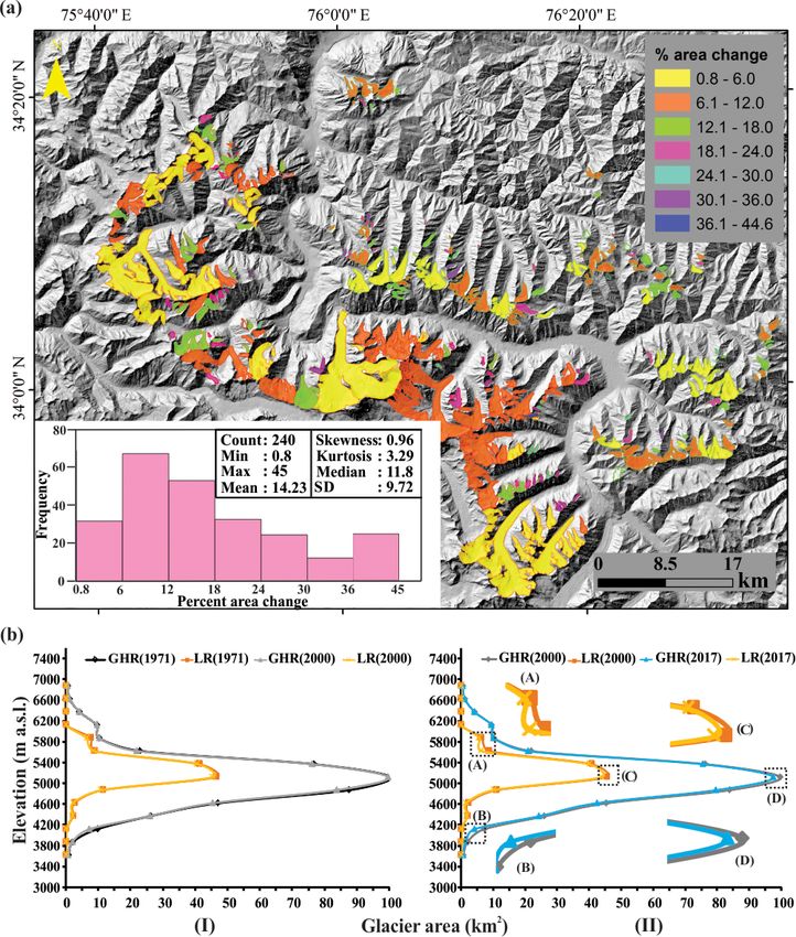
1248                                  A. Shukla et al.: Temporal inventory of glaciers in the Suru sub-basin, western Himalaya

Figure 2. Field photographs of some of the investigated glaciers in the study area captured during the field visits in September 2016 and
2017. Snouts of (a) Pensilungpa, (b) Chilung, (c) Shafat, (e) Kangriz, (f) Sentik and Rantac, (g) Tongul and (h) glacier no. 47. (d) Deglaciated
valley near the Shafat glacier.

Earth Syst. Sci. Data, 12, 1245–1265, 2020                                                  https://doi.org/10.5194/essd-12-1245-2020

A. Shukla et al.: Temporal inventory of glaciers in the Suru sub-basin, western Himalaya                                     1249

2002 (IMD, 2015). However, in order to understand the long-        includes six independent climate variables (mean tempera-
term variability of climatic conditions in the SSB, we have        ture, diurnal temperature range, precipitation, wet-day fre-
utilized the Climate Research Unit (CRU) time series (TS)          quency, vapour pressure and cloud cover). However, in this
version 4.02 data during the period 1901–2017 (Fig. 3; Har-        study monthly mean, minimum and maximum temperature
ris and Jones, 2018). Derived from this data, the annual           and precipitation data are taken into consideration.
mean temperature and precipitation of the SSB for the pe-
riod 1901–2017 was 0.99±0.45 ◦ C and 393±76 mm, respec-            3.2     Methodology adopted
tively. (Standard deviations associated with the mean temper-
ature and precipitation have been italicized throughout the        The following section mentions the methods adopted for data
text.)                                                             extraction, analysis and uncertainty estimation.

3     Datasets and methods                                         3.2.1    Glacier-mapping and estimation of glacier
                                                                            parameters
3.1    Datasets used
                                                                   Initially, the satellite images were co-registered by projec-
The study uses multi-sensor and multi-temporal satellite           tive transformation with sub-pixel accuracy and a root mean
remote-sensing data for extracting the glacier parameters          square error (RMSE) of less than 1 m (Table 1), taking the
for four time periods: 1971/1977, 1994, 2000 and 2017.             Landsat Enhanced Thematic Mapper (ETM+ ) image and the
Details of these time periods are mentioned in Table 1.            ALOS DSM for reference. However, the Corona image was
The study involves six Landsat level-1 terrain correc-             co-registered following a two-step approach: (1) projective
tions (L1Ts), three strips of declassified Corona KH-4B            transformation was performed using nearly 160–250 ground
and one Sentinel multispectral scene, downloaded from              control points (GCPs) and (2) spline adjustment of the im-
USGS Earth Explorer (https://earthexplorer.usgs.gov/, last         age strips (Bhambri et al., 2012). The glaciers were mapped
access: 5 March 2020). Additionally, a global digital sur-         using a hybrid approach, i.e. normalized-difference snow in-
face model (DSM) dataset utilizing the data acquired by the        dex (NDSI) for delineating snow–ice boundaries and manual
Panchromatic Remote-sensing Instrument for Stereo Map-             digitization of the debris cover. Considering that not many
ping (PRISM) on board the Advanced Land Observing Satel-           changes would have occurred in the accumulation region,
lite (ALOS) has also been incorporated (https://www.eorc.          major modifications have been done in the boundaries be-
jaxa.jp/ALOS/en/aw3d30/, last access: 14 August 2019).             low the equilibrium line altitude (ELA; Paul et al., 2017).
ALOS World 3D comprises a fine-resolution DSM (approx.             The glacierets and tributary glaciers contributing to the main
5 m vertical accuracy). It is primarily used for delineating       trunk are considered as a single glacier entity. The NDSI was
the basin boundary and extraction of the snow line altitude        applied to a reference image of Landsat ETM+ using an area
(SLA), elevation range, regional hypsometry and slope.             threshold range of 0.55–0.6. A median filter of kernel size
   The aforementioned satellite images were acquired tak-          3 × 3 was used to remove the noise and very small pixels. In
ing into consideration certain necessary prerequisites such        this manner, glaciers covering a minimum area of 0.01 km2
as peak ablation months (July, August, and September), re-         have been mapped. However, some pixels of frozen water
gional coverage and minimal snow and cloud cover for the           and shadowed regions were manually corrected. Thereafter,
accurate identification and demarcation of the glaciers. Only      the debris-covered part of the glaciers was mapped manu-
three Corona KH-4B strips were available for 1971, which           ally by taking help from the slope and thermal character-
covered the SSB partially, i.e. 40 % of the GHR and 57 %           istics of the glaciers. Furthermore, high-resolution imagery
of the LR glaciers. Therefore, the rest of the glaciers were       from Google Earth™ was also referred to for the accurate
delineated using the Landsat Multispectral Scanner System          demarcation of the glaciers. Identification of the glacier ter-
(MSS) image of the year 1977 (Table 1). Similarly, some of         minus was done based on the presence of certain character-
the glaciers could not be mapped using the Landsat Thematic        istic features at the snout such as ice wall, proglacial lakes
Mapper (TM) image of 27 August 1994 as the image was               and emergence of streams. The length of the glacier was
partially covered with clouds. Therefore, the 26 July 1994         measured along the central flow line (CFL) drawn from the
image of the same sensor was used in order to delineate the        bergschrund to the snout. Fluctuations in the snout position
boundaries of the cloud-covered glaciers.                          (i.e. retreat) of an individual glacier were estimated using the
   Furthermore, long-term climate data have been obtained          parallel line method, in which parallel strips of 50 m spacing
from CRU TS 4.02, which is a high-resolution gridded cli-          are taken on both sides of the CFL. Thereafter, the average
mate dataset obtained from the monthly meteorological ob-          values of these strips intersecting the glacier boundaries were
servations collected at different weather stations of the world.   used to determine the frontal retreat of the glaciers (Shukla
In order to generate this long-term data, station anomalies        and Qadir, 2016; Garg et al., 2017a, b). The mean SLA es-
from 1961 to 1990 are interpolated into 0.5◦ latitude and          timated at the end of the ablation season can be effectively
longitude grid cells (Harris and Jones, 2018). This dataset        used as a reliable proxy for mass balance estimation for a

https://doi.org/10.5194/essd-12-1245-2020                                         Earth Syst. Sci. Data, 12, 1245–1265, 2020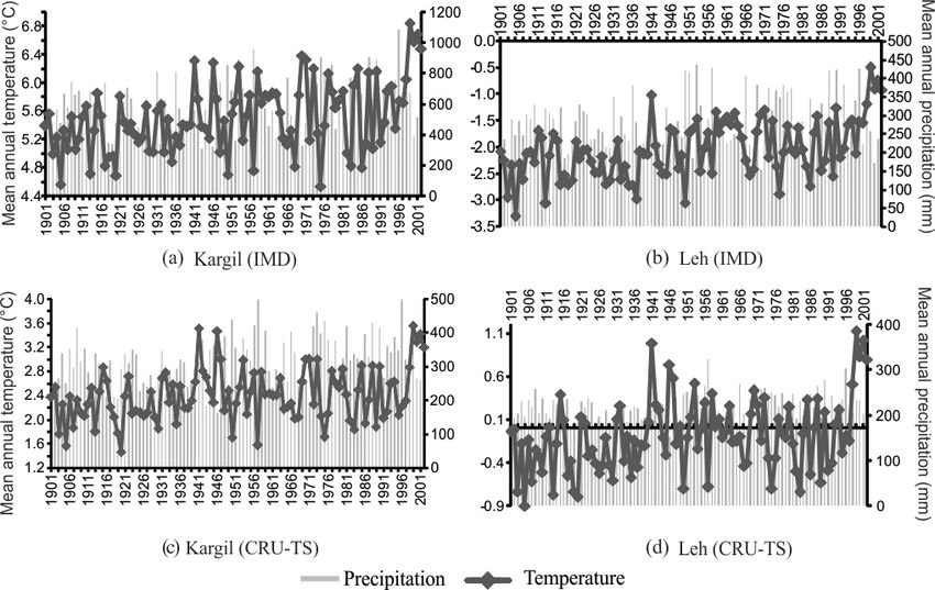
1250                                    A. Shukla et al.: Temporal inventory of glaciers in the Suru sub-basin, western Himalaya

Figure 3. Annual and seasonal variability in the climate data for the period 1901–2017. (a, b, c) Five-year moving average of the mean
annual precipitation (mm) and temperature (◦ C) recorded for five grids covering the glaciers in the entire SSB, GHR and LR (subregions),
respectively, during the period 1901–2017. The dashed light and dark grey lines depict the respective trend lines for precipitation and
temperature conditions during the period 1901–2017. (d, e, f) Monthly mean precipitation and temperature data for the entire SSB, GHR and
LR (subregions), respectively, for the time period 1901–2017.

Table 1. Detailed specifications of the satellite data utilized in the present study. GB: glacier boundaries; DC: debris cover.

 Serial   Satellite sensors   Remarks on          Scene                                           RMSE      Registration   Purpose
 no.      (date of            quality             ID                                                       accuracy (m)
          acquisition)
 1.       Corona KH-4B        Cloud-free          DS1115-2282DA056/DS1115-2282DA055/                 0.1             0.3   Delineation of GB
          (28 Sep 1971)                           DS1115-2282DA054
 2.       LandsatMSS          Cloud-free/peak     LM02_L1TP_159036_19770819_20180422_01_T2/         0.12             10    Delineation of GB,
          (19 Aug 1977/       ablation (17 Aug)                                                                            SLA and DC
          1 Aug 1977)                             LM02_L1TP_159036_19770801_20180422_01_T2
 3.       LandsatTM           Partially cloud-    LT05_L1TP_148036_19940827_20170113_01_T1          0.22              6    Delineation of GB,
          (27 Aug 1994)       covered/peak        /LT05_L1GS_ 148037_19940827_20170113_01_T2                               SLA and DC
                              ablation
 4.       LandsatTM           Seasonal snow       LT05_L1TP_148036_19940726_20170113_01_T1           0.2              6    Delineation of GB
          (26 July 1994)      cover
 5.       LandsatETM+         Cloud-free/peak     LE71480362000248SGS00                                Base image          Delineation of GB,
          (4 Sep 2000)        ablation                                                                                     SLA and DC
 6.       LandsatOLI          Partially cloud-    LC08_L1TP_148036_20170810_01_T1                   0.15             4.5   Delineation of GB
          (25 Jul 2017)       covered/peak                                                                                 and DC, estimation of
                              ablation                                                                                     SLA
 7.       Sentinel MSI        Cloud-free          S2A_MSIL1C_20170920T053641_N0205_R005_            0.12             1.2   Delineation of GB and
          (20 Sep 2017)                           T43SET_20170920T053854                                                   DC
 8.       LISS IV             Cloud-free          183599611                                          0.2            1.16   Accuracy assessment
          (27 Aug 2017)

hydrological year (Guo et al., 2014). The maximum spectral                 as elevation (max and min), regional hypsometry and slope
contrast between snow and ice in the SWIR and NIR bands                    were extracted utilizing the ALOS DSM.
helps in the delineation of the snow line separating the two
facies. The same principle was used in this study to yield the             3.2.2   Analysis of climate variables
snow line. Further, a 15 m buffer was created on both sides
of the snow line to obtain the mean SLA. Other factors such                To ascertain the long-term climate trends in the sub-basin,
                                                                           mean annual temperature (min and max) and precipitation

Earth Syst. Sci. Data, 12, 1245–1265, 2020                                                   https://doi.org/10.5194/essd-12-1245-2020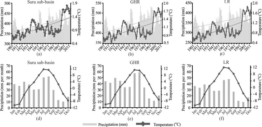
A. Shukla et al.: Temporal inventory of glaciers in the Suru sub-basin, western Himalaya                                      1251

are derived by averaging the mean monthly data of the re-             Though varying in magnitude, the climate data obtained
spective years. Furthermore, seasonal trends are also anal-        from the IMD as well as CRU TS suggest almost simi-
ysed for the winter (November–March) and summer (April–            lar trends of temperature and precipitation during the pe-
October) months. Moreover, the climate variables are as-           riod 1901–2002 for both Kargil and Leh (Fig. 5). During
sessed separately for the ∼ 46-year period (1971–2017),            this period, the annual mean temperature amounted to 5.5 ◦ C
which is the study period of the present research. Further, the    (IMD) and 2.4 ◦ C (CRU TS) in Kargil and −2.04 ◦ C (IMD)
climate dataset was statistically analysed for five grids using    and −0.09 ◦ C (CRU TS) in Leh; the mean annual precipi-
the Mann–Kendall test to obtain the magnitude and signifi-         tation amounted to 589 mm (IMD) and 315 mm (CRU TS)
cance of the trends (Table S2 in the Supplement). The mag-         in Kargil and 279 mm (IMD) and 216 mm (CRU TS) in Leh
nitude of the trends in the time series data was determined        (Fig. 5). We observed that climatic variables show a lower
using Sen’s slope estimator (Sen, 1968). Quantitatively, the       magnitude in the case of the CRU TS as compared to the
temperature and precipitation trends have been assessed here       station data from IMD (except CRU-TS-derived temperature
in absolute terms (determined from Sen’s slope). The change        data recorded for Leh). The possible reason for this differ-
in climate parameters (temperature and precipitation) was          ence between CRU TS and station data can primarily be at-
determined using the following formula:                            tributed to the difference in their nature, with former being
                                                                   point and the latter being gridded data (0.5◦ latitude and lon-
change = (β × L)/M,                                         (1)    gitude grid cells). This analysis aptly brings out the bias in
                                                                   the CRU TS gridded data. Importantly, the comparison shows
where β is Sen’s slope estimator, L is the length of the period,   that the gridded data correctly bring out the temporal trends
and M is the long-term mean.                                       in meteorological data but differ with station data in mag-
   These tests were performed with a confidence level S =          nitude (being lower than the station estimates). This helps
0.1 (90 %), 0.05 (95 %) and 0.01 (99 %), which differed for        us better appreciate the climate variations in the SSB as well
both variables (Table S2). Spatial interpolation of climate        since we learn that the reported temperature and precipitation
data was achieved using the inverse distance weighted (IDW)        changes are probably lower than the actual variations.
algorithm. For this purpose, a total number of 15 CRU TS
grids (in the vicinity of our study area) were taken so as to      3.2.3   Uncertainty assessment
have an ample number of data points in order to achieve ac-
curate results.                                                    This study involves extraction of various glacial parameters
   Further, in order to check data consistency, we have taken      utilizing satellite data with variable characteristics; hence, it
instrument data from the nearest stations of Kargil and Leh        is susceptible to uncertainties which may arise from various
(due to the unavailability of meteorological stations in the       sources. These sources may be locational (LEs), interpreta-
SSB) and compared with the CRU-TS-derived data for the             tional (IEs), classification (CEs) or processing (PEs) errors
entire SSB during the 1901–2002 period (Fig. 4).                   (Racoviteanu et al., 2009; Shukla and Qadir, 2016). In our
   The mean annual temperature pattern of the SSB shows            study, the LEs and PEs may have resulted on account of mis-
a near-negative trend until 1937, with an increase thereafter.     registration of the satellite images and inaccurate mapping,
Similar trends have been observed for Kargil and Leh, de-          respectively. IEs and CEs would have been introduced due to
spite their distant location from the SSB (areal distance of       the misinterpretation of glacier features during mapping. The
Kargil and Leh is ∼ 63 and 126 km, respectively from the           former can be rectified by co-registration of the images and
centre of the SSB). However, it is worth mentioning that all       estimation of the sub-pixel co-registration RMSE (Table 1)
the locations had attained a maximum mean annual tempera-          as well as using standard statistical measures. However, the
ture in 1999 (Suru: 2.02 ◦ C; Kargil: 6.84 ◦ C; Leh: −0.5 ◦ C).    latter can be visually identified and corrected, but exact quan-
We observe an almost similar trend in all the cases (Fig. 4),      tification can be difficult owing to a lack of reliable refer-
with an accelerated warming post-1995/1996. However, the           ence data (field data) in most cases. As a standard procedure
magnitude varies, with a long-term mean annual temperature         for uncertainty estimation, glacier outlines are compared di-
of 0.9, 5.5 and −2.04 ◦ C observed in SSB, Kargil and Leh,         rectly with the ground truth data as acquired using a differ-
respectively (Fig. 4). The possible reason for this difference     ential global positioning system (DGPS) (Racoviteanuet al.,
in their magnitudes could possibly be attributed to their dis-     2008). In this study, a DGPS survey was conducted on the
tinct geographical locations and difference in their nature,       Pensilungpa and Kangriz glaciers at an error of less than
with the former being point data and the latter being the in-      1 cm. Therefore, by comparing the snout position of Pen-
terpolated gridded data.                                           silungpa (2017) and Kangriz (2018) glaciers derived from the
   Furthermore, we have used the station data, obtained            DGPS and Operational Land Imager (OLI) image, an accu-
from the nearest available Indian Meteorological Department        racy of ±23 and ±1.4 m, respectively, was obtained. Further-
(IMD) sites, i.e. Kargil and Leh, and compared with their re-      more, the frontal retreat estimated for the Kangriz glacier us-
spective CRU TS data (mean annual temperature and precip-          ing the DGPS and OLI image is found to be 38.63±47.8 and
itation).                                                          39.98 ± 56.6 m, respectively, during the period 2017–2018.

https://doi.org/10.5194/essd-12-1245-2020                                         Earth Syst. Sci. Data, 12, 1245–1265, 2020
1252                                A. Shukla et al.: Temporal inventory of glaciers in the Suru sub-basin, western Himalaya

Figure 4. Mean annual temperature and precipitation patterns of gridded data derived from the Climate Research Unit (CRU) time series
(TS) in the (a) Suru sub-basin and data recorded by the Indian Meteorological Department (IMD) stations at (b) Kargil and (c) Leh.

Figure 5. Analysis of meteorological (mean annual temperature and precipitation) datasets derived from the Indian Meteorological Depart-
ment (IMD) stations at (a) Kargil and (b) Leh and the respective (c) Kargil and (d) Leh gridded data obtained from the Climate Research
Unit (CRU) time series (TS).

In this study, high-resolution Linear Imaging Self Scanner            areal uncertainty estimated are given in Table 2.
(LISS) IV imagery (spatial resolution of 5.8 m) is also used
for validating the glacier-mapping results for the year 2017          Area change uncertainty (UA ) = 2 × U T × x,                  (3)
(Table 1). Glaciers of varying dimensions and distribution of
                                                                      where x is the spatial resolution of the sensor.
debris cover were selected for this purpose. The area- and
                                                                         Area-mapping uncertainty was estimated using the buffer
length-mapping accuracy for these selected glacier bound-
                                                                      method, in which a buffer size equal to the registration error
aries (G-1, G-2, G-3, G-13, G-41, G-209, G-215, G-216, G-
                                                                      of the satellite image was taken into consideration (Bolch et
220, G-233) was found to be 3 % and 0.5 %, respectively.
                                                                      al., 2012; Garg et al., 2017a, b). Using this method, the error
   The multi-temporal datasets were assessed for glacier
                                                                      was estimated to be 0.48, 27.2, 9.6 and 3.41 km2 for the 1971
length and area change uncertainty as per the methods given
                                                                      (Corona), 1977 (MSS), 1994 (TM) and 2017 (OLI) images,
by Hall et al. (2003) and Granshaw and Fountain (2006). The
                                                                      respectively. Since the debris extents were delineated within
following formulations (Hall et al., 2003) were used for esti-
                                                                      the respective glacier boundaries, the proportionate errors are
mation of the said parameters:
                                                                      likely to have propagated in debris cover estimations, which
                              p
terminus uncertainty (UT ) = a 2 + b2 + σ,                (2)         were estimated accordingly (Garg et al., 2017b).
                                                                         Uncertainty in SLA estimation needs to be reported in the
where a and b are the pixel resolution of image 1 and 2, re-          X, Y and Z directions. In this context, error in the X and Y
spectively, and σ is the registration error. The terminus and         directions should be equal to the distance taken for creating

Earth Syst. Sci. Data, 12, 1245–1265, 2020                                             https://doi.org/10.5194/essd-12-1245-2020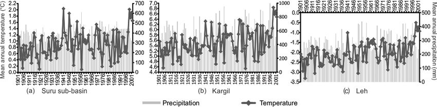
A. Shukla et al.: Temporal inventory of glaciers in the Suru sub-basin, western Himalaya 1253
Table 2. Terminus and area change uncertainty associated with the satellite dataset as defined by Hall et al. (2003). UT : terminus uncertainty;
UA : area change uncertainty; x: spatial resolution; σ : registration accuracy.
Serial Satellite Terminus
p uncertainty Area change uncertainty
no. sensor (UT ) = a 2 + b2 + σ UA = 2UT × x
1. Corona KH-4B 3.12 m 0.00007 km2
2. Landsat MSS 123.13 m 0.03 km2
3. Landsat TM 41.42 m 0.003 km2
4. Landsat ETM+ 48.42 m 0.003 km2
5. Landsat OLI 46.92 m 0.003 km2
the buffer on either side of the snow line demarcating the Categorization of the glaciers based on this criteria shows
snow and ice facies. Since the buffer size taken in this study their proportion in the glacierized basin as 43 % (CGs), 40 %
was 15 m, the error in the X and Y direction was considered (PDGs) and 17 % (HDGs). A majority of the glaciers in
to be ±15 m. However, uncertainty in the Z direction would the sub-basin are north-facing (N/NW/NE: 71 %), followed
be similar to the ALOS DSM, i.e. ±5 m. by south (S/SW/SE: 20 %), with very few oriented in other
(E/W: 9 %) directions (Fig. 1a). The mean elevation of the
glaciers in the SSB is 5134.8 ± 225 m a.s.l., with an aver-
4 Results
age elevation of 5020 ± 146 and 5260 ± 117 m a.s.l. in the
The present study involved the creation of a glacier inven- GHR and LR, respectively. The mean slope of the glaciers
tory for the year 2017 and the estimation of glacier (area, is 24.8◦ ± 5.8◦ and varies from 24◦ ± 6◦ to 25◦ ± 6◦ in the
length, debris cover and SLA) parameters for four differ- GHR and LR, respectively, while the percentage distribution
ent time periods. For detailed insight, the variability of the of the glaciers shows that nearly 80 % of the LR glaciers have
glacier parameters has also been evaluated on a decadal scale, a steeper slope (20–40◦ ) as compared to the GHR glaciers
in which the total time period has been subdivided into three (57 %).
time frames: 1971–1994 (23 years), 1994–2000 (6 years) and
2000–2017 (17 years). 4.2 Area changes
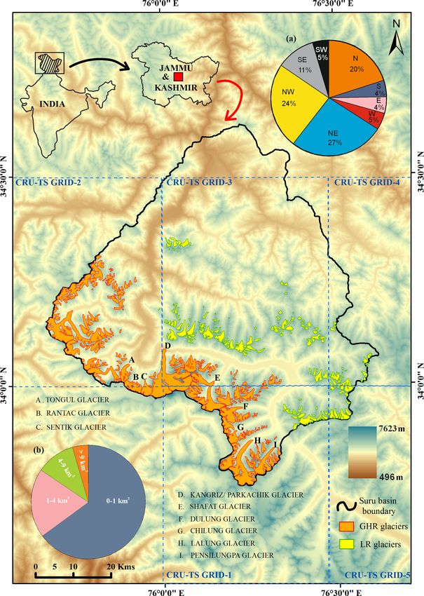
The glaciated area reduced from 513 ± 14 km2 (1971) to
4.1 Basin statistics 481 ± 3.4 km2 (2017), exhibiting an overall deglaciation of
32 ± 9 km2 (6 ± 0.02 %) during the period 1971–2017. The
The SSB covers an area of ∼ 4429 km2 . In 1971, the sub- percentage of area loss of the individual glaciers ranges be-
basin had around 240 glaciers, with 126 glaciers located in tween 0.8 % (G-50; Parkachik glacier) and 45 % (G-81), with
the GHR and 114 in the LR, which remained the same until a majority of the glaciers undergoing an area loss in the range
2000. However, a major disintegration of glaciers took place of 6 %–12 % during the period 1971–2017 (Fig. 6a).
during the period 2000–2017, which resulted in the break- The results show that the highest pace of deglaciation is
down of about 12 glaciers into smaller glacierets. The recent observed in the periods 1994–2000 (0.95 ± 0.005 km2 a−1 )
(2017) distribution of the glaciers in the GHR and LR is 130 and 2000–2017 (0.86 ± 0.0002 km2 a−1 ), followed by 1971–
and 122, respectively (Table S1). The overall glacierized area 1994 (0.5 ± 0.001 km2 a−1 ) (Fig. S1a in the Supplement).
is ∼ 11 %, with the size and length of the glaciers varying Within the SSB, glaciers in the LR exhibit higher deglacia-
from 0.01 to 53.1 km2 and 0.15 to 16.34 km, respectively. tion (7±7.2 %) as compared to GHR (6±2 %) during the pe-
Within the sub-basin, the size range of glaciers in the GHR riod 1971–2017. Apart from deglaciation, G-50 also showed
and LR varies from 0.01 (G-115) to 53.1 km2 (G-50) and an increase in glacier area during the period 1994–2000;
0.03 (G-155/165) to 6.73 km2 (G-209), respectively. Con- however, this increase was insignificant.
sidering this, glaciers have been categorized as small (0–
7 km2 /0–2 km), medium (7–15 km2 /2–7 km) and large (>
4.3 Length changes
15 km2 / > 7 km). Based on the size distribution, small (com-
prising all the LR and some GHR glaciers), medium and Fluctuations in the glacier snout have been estimated during
large glaciers occupy 47 %, 15 % and 38 % of the glacier- the period 1971–2017, and it is observed that nearly all the
ized sub-basin, respectively. Depending on the percentage glaciers have retreated during the said period; however the re-
of area occupied by the supraglacial debris out of the to- treat rates vary considerably. The overall average retreat rate
tal glacier area, the glaciers have been categorized as clean of the glaciers is observed to be 4.3 ± 1.02 m a−1 during the
(CGs: 0 %–25 %), partially debris-covered (PDGs: 25 %– period 1971–2017. The percentage of length change of the
50 %) and heavily debris-covered (HDGs: > 50 %) glaciers. glaciers ranges between 0.9 % and 47 %, with the majority
https://doi.org/10.5194/essd-12-1245-2020 Earth Syst. Sci. Data, 12, 1245–1265, 2020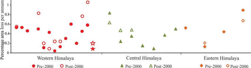
1254                                 A. Shukla et al.: Temporal inventory of glaciers in the Suru sub-basin, western Himalaya

Figure 6. (a) Percentage of area loss of the glaciers in the SSB during the period 1971–2017. Frequency distribution histogram depicting
that the majority of the glaciers have undergone an area loss in the range of 6 %–12 %. (b) Hypsometric distribution of glacier area in the
GHR and LR regions during the periods (I) 1971–2000 and (II) 2000–2017. (A), (B), (C) and (D) insets in (II) show the significant change
in area at different elevation ranges of the GHR and LR glaciers.

of the glaciers retreating in the range of 6 %–14 % during the          4.4   Debris cover changes
period 1971–2017 (Fig. 7).
                                                                        The results show an overall increase in debris cover extent of
   Decadal observations reveal the highest rate of retreat be-
                                                                        62 % (∼ 37 ± 0.002 km2 ) in the SSB glaciers during the pe-
tween 1994 and 2000 (7.37 ± 8.6 m a−1 ) followed by 2000–
                                                                        riod 1971–2017. Decadal variations exhibit the maximum in-
2017 (4.66 ± 1.04 m a−1 ), and the lowest between 1971 and
                                                                        crease in the debris cover of approximately 19±0.00004 km2
1994 (3.22 ± 2.3 m a−1 ) (Fig. S1b). Moreover, the average
                                                                        (24 %) between 2000 and 2017 followed by an increase of
retreat rate in the GHR and LR glaciers was observed to be
                                                                        13 ± 0.0001 km2 (20 %) and 5 ± 0.0001 km2 (9 %) between
5.4 ± 1.04 and 3.3 ± 1.04 m a−1 , respectively, during the pe-
                                                                        1994 and 2000 and between 1971 and 1994, respectively
riod 1971–2017. The retreat rate of individual glaciers varied
                                                                        (Fig. S1c). However, GHR and LR glaciers show an over-
from 0.72 ± 1.02 m a−1 (G-114) to 28.92 ± 1.02 m a−1 (G-7,
                                                                        all increase of debris cover extent of 59 % and 73 %, respec-
i.e. Dulung glacier) during the period 1971–2017. Further-
                                                                        tively, during the entire study period, i.e. 1971–2017.
more, the Kangriz glacier (G-50) also showed advancement
during the period 1994–2000 by 5.23 ± 8.6 m a−1 .

Earth Syst. Sci. Data, 12, 1245–1265, 2020                                               https://doi.org/10.5194/essd-12-1245-2020
A. Shukla et al.: Temporal inventory of glaciers in the Suru sub-basin, western Himalaya 1255
Figure 7. Percentage of length change of the glaciers in the SSB during the period 1971–2017. Frequency distribution histogram showing
that majority of the glaciers have undergone length change in the range of 6 %–14 %.
4.5 SLA variations 5.1 Glacier variability in the Suru sub-basin: a
comparative evaluation
The mean SLA shows an average increase of 22 ± 60 m dur-
ing the period 1977–2017. On the decadal scale, SLA varia-
tions showed the highest increase (161±59 m) between 1994 Basin statistics reveal that in the year 2000, the SSB
and 2000 with a considerably lower increase (8 ± 59 m) be- comprised 240 glaciers covering an area of approximately
tween 1977 and 1994 and a decrease (150 ± 60 m) between 496 km2 . However, these figures differ considerably from the
2000 and 2017. Amongst the four time periods (1977, 1994, previously reported studies in this particular sub-basin, with
2000 and 2017) used for mean SLA estimation, the highest the total number of glaciers and the glacierized area varying
SLA is noted in 2000 (5158 ± 65 m a.s.l.) and the lowest in from 284 and 718.86 km2 (Sangewar and Shukla, 2009) to
1977 (4988 ± 65 m a.s.l.) (Fig. S1d). 110 and 156.61 km2 (SAC, 2016), respectively. In contrast,
During the period 1977–2017, the average SLA of the LR the glacierized area is found to be less than – yet compara-
glaciers is observed to be relatively higher (5155 ± 7 m a.s.l.) ble with – the RGI boundaries (550.88 km2 ). Furthermore,
as compared to the GHR glaciers (4962 ± 9 m a.s.l.). In con- debris cover distribution of the glaciers in 2000 is observed
trast, an overall rise in mean SLA was noted in the GHR to be ∼ 16 % in the present study, which is almost half of
(49±69 m), while a decrease was observed in the LR glaciers that reported in the RGI (30 %). Variability in these figures
(18 ± 45 m) during the time frame of 1977–2017. is possibly due to the differences in the mapping techniques,
thereby increasing the risk of systematic error. Moreover, due
to the involvement of different analysts in the latter, the re-
5 Discussion
sults may more likely suffer from random errors.
Results from this study reveal an overall deglaciation of
The present study reports detailed temporal inventory data of
the glaciers in the SSB at an annual rate of ∼ 0.1 ± 0.0004 %
the glaciers in the SSB considering multiple glacier param-
during the period 1971–2017. This quantum of area loss is
eters, evaluates the ensuing changes for ascertaining the sta-
comparatively less than the average annual rate of 0.4 % re-
tus of the glaciers and relates them to climate variability and
ported in the western Himalaya (Table S3). However, our
other inherent terrain characteristics. The results suggest an
results are comparable with Birajdar et al. (2014), Chand
overall degeneration of the glaciers with pronounced spatial
and Sharma (2015) and Patel et al. (2018) and differ con-
and temporal heterogeneity in response.
siderably with other studies in the western Himalaya (Ta-
https://doi.org/10.5194/essd-12-1245-2020 Earth Syst. Sci. Data, 12, 1245–1265, 20201256 A. Shukla et al.: Temporal inventory of glaciers in the Suru sub-basin, western Himalaya ble S3). Period-wise deglaciation varied from 0.1 ± 0.0007 basin (Raina, 2009), Doda valley (Shukla and Qadir, 2016), to 0.2 ± 0.005 % a−1 between 1971 and 2000 as well as be- Chandra–Bhaga basin (Pandey and Venkataraman, 2013) and tween 2000 and 2017, respectively. This result is in line with Zanskar basin (Pandey et al., 2011). However, these studies the recent findings by Maurer et al. (2019), who suggest may not sufficiently draw a generalized picture of glacier re- a higher average mass loss post-2000 (−0.43 m w.e. a−1 ), cession in the Himalayan region. which is almost double the rate reported between 1975 and 2000 (−0.22 m w.e. a−1 ) for the entire Himalaya. 5.2 Spatio-temporal variability in the climate data A comparison of the deglaciation rates of the glaciers within the western Himalayan region reveals considerable Climatic fluctuations play a crucial role in understanding heterogeneity therein (Table S3). It is observed that the glacier variability. In this regard, the CRU TS 4.02 dataset Karakoram Himalayan glaciers in particular had been los- helped in delineating the long-term fluctuations in the tem- ing area until 2000 at an average rate of 0.09 % a−1 , with perature and precipitation records. an increase in area thereafter of ∼ 0.05 % a−1 (Liu et al., 2006; Minora et al., 2013; Bhambri et al., 2013). However, 5.2.1 Basin-wide climate variability glaciers in the GHR and Trans-Himalayan range have been deglaciating with higher average annual rates of 0.4 % a−1 During an entire duration of 116 years, i.e. from 1901 to and 0.6 % a−1 , respectively, during the period 1962–2016 2017, the maximum mean annual temperature is observed (Kulkarni et al., 2007, 2011; Rai et al., 2013; Chand and in 2016 (3.23 ◦ C) and minimum in 1957 (−0.51 ◦ C). The Sharma, 2015; Mir et al., 2017; Schmidt and Nuesser, 2017; mean annual temperature shows an almost uniform trend un- Chudley et al., 2017; Patel et al., 2018; Das and Sharma, til 1996, with a pronounced rise thereafter until 2005/2006 2018). In contrast to these studies, deglaciation rates in (Fig. 3a, b, c). The globally averaged combined land and the SSB, which comprises glaciers in the GHR as well as ocean surface temperature data of the 1983–2012 period the LR, have varied from 0.1 % a−1 (GHR) to 0.2 % a−1 are considered to be the warmest 30-year period in the last (LR) (present study). These results evidently depict that 1400 years (IPCC, 2013). This unprecedented rate of warm- the response of the SSB glaciers is transitional between ing is primarily attributed to the rapid scale of industrializa- the Karakoram Himalayan and GHR glaciers. Period-wise tion, increase in regional population and anthropogenic ac- area loss of the glaciers in the Himalayan region suggests tivities prevalent during this time period (Bajracharya et al., maximum average deglaciation of eastern (0.49 % a−1 ) fol- 2008; IPCC, 2013). Thus, one of the probable reasons for lowed by central (0.36 % a−1 ) and western (0.35 % a−1 ) Hi- this sudden increase in temperature pattern is possibly due to malayan glaciers before 2000. Contrarily, after 2000, the the greenhouse effect from enhanced emission of black car- central Himalayan glaciers deglaciated at the maximum rate bon in this region (by 61 %) from 1991 to 2001. Evidence of (0.52 % a−1 ) followed by western (0.46 % a−1 ) and eastern incessant increase in temperature during the 1990s has also (0.44 % a−1 ) Himalayan glaciers (Fig. 8). Though these rates been observed (through chronology of the Himalayan pine) reflect the possible trend of deglaciation in the Himalayan from the contemporaneous surge in tree growth rate (Singh terrain, any conclusion drawn would be biased due to insuf- and Yadav, 2000). In fact, 50 % of the years since 1970 have ficient data, particularly in the eastern and central Himalaya. experienced considerably high solar irradiance and warm In this study, we found an overall average retreat rate phases of El Niño–Southern Oscillation, which is possibly of 4.3 ± 1.02 m a−1 during the period 1971–2017. However, one of the reasons for the considerable rise in temperature the average retreat rates of seven glaciers in the SSB re- throughout the Himalaya (Shekhar et al., 2017). The maxi- ported by Kamp et al. (2011) are found to be nearly twice mum mean annual precipitation is noted in 2015 (615 mm) (24 m a−1 ) of those found in this study (10 m a−1 ). The com- and the minimum in 1946 (244 mm). However, the mean an- paratively higher retreat rates in the former might be due to nual precipitation followed a similar trend until 1946, with the consideration of different time frames. The average re- an increase thereafter (Fig. 3a, b, c). Besides these general treat rates in other basins of the western Himalaya are also trends in temperature and precipitation, an overall absolute found to be higher (7.8 m a−1 ) in the Doda valley (Shukla and increase in the mean annual temperature (Tmax and Tmin ) Qadir, 2016), 8.4 m a−1 in the Liddar valley (Murtaza and and precipitation data has been noted as 0.77 ◦ C (0.25 and Romshoo, 2015), 15.5 m a−1 in the Chandra–Bhaga basin 1.3 ◦ C) and 158 mm, respectively, during the period 1901– (Pandey and Venkataraman, 2013) and 19 m a−1 in the Baspa 2017. These observations suggest an enhanced increase in basin (Mir et al., 2017). These results show lower average re- Tmin by nearly 5 times as compared to the Tmax along with a treat rates of the glaciers in the SSB as compared to the other simultaneous increase in the precipitation during the period studies in the western Himalaya. 1901–2017. The observed average retreat rates between 2000 and Seasonal variations reveal monthly mean temperatures 2017 (4.6 ± 1.02 m a−1 ) are found to be nearly twice of and precipitation of 6.7 ◦ C and 1071 mm during summer those noted between 1971 and 2000 (2 ± 1.7 m a−1 ). Similar (April–October) and −6.9 ◦ C and 890 mm during winter higher retreat rates post-2000 have been reported in the Tista (November–March) recorded during the 1901–2017 period. Earth Syst. Sci. Data, 12, 1245–1265, 2020 https://doi.org/10.5194/essd-12-1245-2020
A. Shukla et al.: Temporal inventory of glaciers in the Suru sub-basin, western Himalaya                                                 1257

Figure 8. Annual rate of area loss of glaciers (in per cent) in three major sections of the Himalaya before and after 2000. Details of the same
have been mentioned in Table S3. Results from the present study have been star-marked in the western Himalaya.

The maximum monthly mean temperature and precipitation                    (448 mm) and grid 1 (442 mm) experienced wetter climate as
have been observed in July (11.8 ◦ C/50.4 mm) and August                  compared to grid 4 (383 mm), grid 3 (373 mm) and the min-
(11.4 ◦ C/52 mm) during the period 1901–2017, suggesting                  imum in grid 5 (318 mm). These observations suggest that
that they were the warmest and wettest months, while Jan-                 GHR glaciers have been experiencing a warmer and wetter
uary is noted to be the coldest (−10.4 ◦ C) and November                  climate (1.03 ◦ C/445 mm) as compared to the LR glaciers
(10.3 mm) to be the driest month in the duration of 116 years             (0.96 ◦ C/358 mm) (Fig. 3e, f). These observations clearly
(Fig. 3d, e, f). Summer and winter mean annual temperatures               show that local climate variability does exist in the basin for
and precipitation have increased significantly by an average              the entire duration of 116 years (Fig. 9).
of 0.74/1.28 ◦ C and 85/72 mm, respectively, during the pe-
riod 1901–2017. These values reveal a relatively higher rise              5.3     Glacier changes: impact of climatic and other
in winter average temperature in contrast to the summer.                          plausible factors
However, enhanced increase in Tmin (1.8 ◦ C) during winter
and Tmax (0.78 ◦ C) during summer has also been observed                  The alterations in the climatic conditions discussed in
during the 1901–2017 time period. The relatively higher rise              Sect. 5.2 would in turn influence the glacier parameters, but
in the winter temperature (particularly Tmin ) and precipita-             these would vary with time. This section correlates the cli-
tion possibly suggests that the form of precipitation might               matic and other factors (elevation range, regional hypsome-
have changed from solid to liquid during this particular time             try, slope, aspect and proglacial lakes) with the variations in
span. A similar increase in the winter temperature has also               the glacier parameters.
been reported from the NW Himalaya during the 20th cen-
tury (Bhutiyani et al., 2007).                                            5.3.1    Impact of climatic factors
   In contrast to the long-term climate trends, we have
also analysed the climate data for the study period, i.e.                 An overall degenerating pattern of the glaciers in the SSB is
1971–2017. An overall increase in the average temperature                 observed during the period 1971–2017, with deglaciation of
(0.3 ◦ C), Tmax (0.45 ◦ C), Tmin (1.02 ◦ C) and precipitation             32 ± 9 km2 (6 ± 0.02 %). In the same duration, the glaciers
(213 mm) is observed. Meanwhile, an enhanced increase in                  have also retreated by an average 199 ± 46.9 m (retreat rate:
winter Tmin (1.7 ◦ C) and summer Tmax (0.45 ◦ C) is observed.             4.3 ± 1.02 m a−1 ) along with an increase in the debris cover
These findings aptly indicate the important role of winter                of ∼ 62 %. The observed overall degeneration of the glaciers
Tmin and summer Tmax in the SSB.                                          possibly resulted from the warming of climatic conditions
                                                                          during this particular time frame. The conspicuous degener-
5.2.2   Local climate variability
                                                                          ation of these glaciers might have led to an increased melt-
                                                                          ing of the glacier surface, which in turn would have unveiled
Apart from these generalized climatic variations, grid-wise               the englacial debris cover and increased its coverage in the
analysis of the meteorological parameters reveals the ex-                 ablation zone (Shukla et al., 2009; Scherler et al., 2011).
istence of local climate variability within the sub-basin                 A more enhanced degeneration of the glaciers has been
(Figs. 3, 9).                                                             noted between 2000 and 2017 (0.85 ± 0.005 km2 a−1 ) than
   Observations indicate that the glaciers covered in grid                between 1971 and 2000 (0.59 ± 0.005 km2 a−1 ). Moreover,
4 have been experiencing warmer climatic regimes with a                   nearly 12 glaciers have shown disintegration into glacierets
maximum annual mean temperature of 1.69 ◦ C as compared                   after 2000. These observations may be attributed to the rel-
to the other glaciers in the region (grid 2: 1.4 ◦ C; grid 5:             atively higher annual mean temperature (1.68 ◦ C) during the
0.74 ◦ C; grid 1: 0.65 ◦ C; grid 3: 0.45 ◦ C). Spatial variabil-          former as compared to the period 1971–2000 (0.89 ◦ C). Con-
ity in annual mean precipitation data reveals that grid 2                 comitant to the maximum glacier degeneration during the pe-

https://doi.org/10.5194/essd-12-1245-2020                                                  Earth Syst. Sci. Data, 12, 1245–1265, 2020
1258 A. Shukla et al.: Temporal inventory of glaciers in the Suru sub-basin, western Himalaya Figure 9. Spatial variation in meteorological data recorded for 15 grids in the SSB during the period 1901–2017. Map showing the long-term mean annual (a) temperature (◦ C) and (b) precipitation (mm) data within the sub-basin, suggesting the existence of significant local climate variability in the region. Glacier boundaries are shown as GHR (red) and LR (yellow). riod 2000–2017, debris cover extent has also increased more gen, 2014). SLAs are amongst the dynamic glacier parame- (24 %) as compared to 1971–2000 (16 %). The enhanced de- ters that alter seasonally and annually, indicating their direct generation of the glaciers between 2000 and 2017 might have dependency on climatic factors such as temperature and pre- facilitated an increase in the distribution of supraglacial de- cipitation. In the present study, the mean SLA has gone up bris cover. A transition from CGs to PDGs has also been no- by an average 22 ± 60 m during the period 1977–2017. This ticed, which resulted from an increase in the debris cover rise in SLA is synchronous with the increase in mean annual percentage over nearly 99 glaciers. A conversion from PDGs temperature of 0.43 ◦ C. Moreover, the maximum rise in SLA to HDGs (39) and from CGs to HDGs (2) has also oc- between 1994 and 2000 is contemporaneous with the rise in curred. Furthermore, most of these transitions occurred be- temperature of 0.64 ◦ C during this time period. tween 2000 and 2017, which confirms the maximum degen- Further, in order to understand the regional heterogene- eration of the glaciers during this particular period. ity in glacier response within the sub-basin, parameters of It is observed in our study that smaller glaciers have the GHR and LR glaciers are analysed separately for four deglaciated more (4.13 %) than the medium- (1.08 %) and different time periods and correlated with the climatic vari- larger-sized (1.03 %) glaciers during the period 1971–2017 ables. The LR glaciers were found to have deglaciated more (Fig. S2). This result depicts an enhanced sensitivity of the (7.2 %) as compared to the GHR glaciers (5.9 %). Similarly, smaller glaciers to climate change (Bhambri et al., 2011; more debris cover is found to have accumulated over the LR Basnett et al., 2013; Ali et al., 2017). A similar pattern of (73 %) glaciers as compared to the GHR (59 %) glaciers be- glacier degeneration is noted between 1971 and 2000, with tween 1971 and 2017. This result shows that the relatively smaller glaciers deglaciating more (5 %) as compared to the cleaner (LR) glaciers tend to deglaciate more and accumu- medium-sized (3 %) and larger (1 %) ones. However between late more debris as compared to the debris-covered and par- 2000 and 2017, medium glaciers showed slightly greater de- tially debris-covered glaciers (GHR glaciers) (Bolch et al., generation (3.9 %) as compared to the smaller (3.7 %) and 2008; Scherler et al., 2011). Moreover, the increase in mean larger ones (1.5 %). We have also observed the maximum annual temperature in the LR (0.3 ◦ C) is slightly greater than length change for smaller glaciers (8 %) in comparison to in the GHR (0.25 ◦ C) during the period 1971–2017, thus ex- medium (5 %) and large glaciers (3 %). These results indicate hibiting a positive correlation with deglaciation and debris that the snout retreats are commonly associated with small- cover distribution in these regions. We also observed that the and medium-sized glaciers (Mayewski et al., 1980). glacier area, length and debris cover extent of the LR glaciers Temporal and spatial variations in SLAs are an indica- show a good correlation with winter Tmin and average pre- tor of ELAs, which in turn provide direct evidence related cipitation as compared to the GHR glaciers (Table 3). This to the change in climatic conditions (Hanshaw and Bookha- shows that both temperature and precipitation influence the Earth Syst. Sci. Data, 12, 1245–1265, 2020 https://doi.org/10.5194/essd-12-1245-2020
You can also read