Recent ozone trends in the Chinese free troposphere: role of the local emission reductions and meteorology
←
→
Page content transcription
If your browser does not render page correctly, please read the page content below
Atmos. Chem. Phys., 21, 16001–16025, 2021
https://doi.org/10.5194/acp-21-16001-2021
© Author(s) 2021. This work is distributed under
the Creative Commons Attribution 4.0 License.

Recent ozone trends in the Chinese free troposphere:
role of the local emission reductions and meteorology
Gaëlle Dufour1 , Didier Hauglustaine2 , Yunjiang Zhang2,a , Maxim Eremenko3 , Yann Cohen2 , Audrey Gaudel4 ,
Guillaume Siour3 , Mathieu Lachatre5,b , Axel Bense3 , Bertrand Bessagnet6,c , Juan Cuesta3 , Jerry Ziemke7,8 ,
Valérie Thouret9 , and Bo Zheng10
1 Université  de Paris and Univ Paris Est Creteil, CNRS, LISA, 75013 Paris, France
2 Laboratoire   des Sciences du Climat et de l’Environnement (LSCE), UMR 8212, CEA-CNRS-UVSQ, Gif-sur-Yvette, France
3 Univ Paris Est Creteil and Université de Paris, CNRS, LISA, 94010 Créteil, France
4 CIRES, University of Colorado/NOAA Chemical Sciences Laboratory, Boulder, CO, USA
5 LMD/IPSL, École Polytechnique, Institut Polytechnique de Paris, ENS, PSL Université, Sorbonne Université,

CNRS, Palaiseau, France
6 Ecole Polytechnique, Institut Polytechnique de Paris, ENS, PSL Université, Sorbonne Université, CNRS,

91128 Palaiseau, France
7 NASA Goddard SpaceFlight Center, Greenbelt, Maryland, USA
8 Morgan State University, Baltimore, Maryland, USA
9 Laboratoire d’Aérologie, Université de Toulouse, CNRS, UPS, Toulouse, France
10 Institute of Environment and Ecology, Tsinghua Shenzhen International Graduate School, Tsinghua University,

Shenzhen 518055, China
a now at: School of Environmental Science and Engineering, Nanjing University of Information Science and Technology,

Nanjing 210044, China
b now at: ARIA Technologies, 8–10 Rue de la Ferme, 92100 Boulogne-Billancourt, France
c now at: European Commission, Joint Research Centre (JRC), Ispra, Italy

Correspondence: Gaëlle Dufour (gaelle.dufour@lisa.ipsl.fr)

Received: 7 June 2021 – Discussion started: 5 July 2021
Revised: 23 September 2021 – Accepted: 23 September 2021 – Published: 28 October 2021

Abstract. Free tropospheric ozone (O3 ) trends in the Cen-        with the model, we evaluate, at 60 % and 52 %, the contri-
tral East China (CEC) and export regions are investigated for     bution of the Chinese anthropogenic emissions to the trend
2008–2017 using the IASI (Infrared Atmospheric Sounding           in the lower and upper free troposphere, respectively. The
Interferometer) O3 observations and the LMDZ-OR-INCA              second main contribution to the trend is the meteorological
model simulations, including the most recent Chinese emis-        variability (34 % and 50 %, respectively). These results sug-
sion inventory. The observed and modelled trends in the           gest that the reduction in NOx anthropogenic emissions that
CEC region are −0.07 ± 0.02 and −0.08 ± 0.02 DU yr−1 , re-        has occurred since 2013 in China led to a decrease in ozone
spectively, for the lower free troposphere (3–6 km column)        in the Chinese free troposphere, contrary to the increase in
and −0.05 ± 0.02 and −0.06 ± 0.02 DU yr−1 , respectively,         ozone at the surface. We designed some tests to compare the
for the upper free troposphere (6–9 km column). The sta-          trends derived by the IASI observations and the model to in-
tistical p value is smaller to 0.01 for all the derived trends.   dependent measurements, such as the In-service Aircraft for
A good agreement between the observations and the model           a Global Observing System (IAGOS) or other satellite mea-
is also observed in the region, including the Korean Penin-       surements (Ozone Monitoring Instrument (OMI)/Microwave
sula and Japan and corresponding to the region of pollution       Limb Sounder (MLS)). These comparisons do not confirm
export from China. Based on sensitivity studies conducted         the O3 decrease and stress the difficulty in analysing short-

Published by Copernicus Publications on behalf of the European Geosciences Union.
16002                                                  G. Dufour et al.: Recent ozone trends in the Chinese free troposphere

term trends using multiple data sets with various sampling         show the ability to inform on pollution events in the North
and the risk of overinterpreting the results.                      China Plain (NCP). The IASI + GOME2 O3 product shows
                                                                   a better ability to reproduce ozone surface concentrations,
                                                                   with good comparisons with surface measurements in Japan
                                                                   (Cuesta et al., 2018). Despite this encouraging partial sen-
1   Introduction                                                   sitivity to the surface or boundary layer ozone, satellite ob-
                                                                   servations such as IASI are mostly suited to probe free tro-
Tropospheric ozone is a harmful pollutant close to the surface     pospheric ozone. IASI is, however, able to separate, at least
impacting human health and ecosystems (Lelieveld et al.,           partly, the information from the lower and the upper tropo-
2015; Monks et al., 2015). Tropospheric ozone is also a            sphere with a maximum of sensitivity between 3 and 6 km
short-lived climate forcer with an impact on surface temper-       (Dufour et al., 2010, 2012, 2015). Based on the IASI ob-
ature that is greatest in the upper troposphere lower strato-      servations, Dufour et al. (2018) discuss lower tropospheric
sphere (UTLS) and then contributes to climate change (Riese        O3 trends (surf–6 km) over the NCP for the 2008–2016 pe-
et al., 2012). The recent Tropospheric Ozone Assessment Re-        riod and associate driving factors using a multivariate regres-
port (TOAR) has stated that free tropospheric O3 increased         sion model. They show that the O3 trend derived from IASI
during industrial times and the last few decades (Gaudel           is negative (−0.24 DU yr−1 or −1.2 % yr−1 ) and explained
et al., 2018; Tarasick et al., 2019). At the surface, the trends   by large-scale dynamical processes, such as El Niño and
depend on the following considered regions: a decrease is ob-      changes in precursors emissions, that have occurred since
served during summertime in North America and in Europe            2013. The hypothesis to explain the negative impact of pre-
and an increase is observed in Asia (e.g. Gaudel et al., 2018,     cursors reduction compared to the positive one at the sur-
2020). However, conclusions are more difficult to draw for         face is related to the chemical regime turning from VOC lim-
the recent trends of tropospheric ozone. In addition to the sta-   ited at the surface to NOx limited in altitude. In this study,
tistical robustness of these trends, Gaudel et al. (2018) point    we examine the ability of IASI to derive free tropospheric
out inconsistencies between satellite trends derived from ul-      ozone trends in China by comparison with the state-of-the-
traviolet (UV) sounders, which show mainly positive trends         art global chemistry climate model LMDZ-OR-INCA for the
(e.g. Cooper et al., 2014; Ziemke et al., 2019) and infrared       2008–2017 period. Satellite observations and the model are
(IR) sounders, which show mainly negative trends (Wespes           evaluated using independent observations (surface measure-
et al., 2017).                                                     ments, In-service Aircraft for a Global Observing System
   In China and Central East China (CEC), one of the most          (IAGOS) aircraft measurements, and ozonesondes). We use
polluted regions worldwide (e.g. Wang et al., 2017; Fan et al.,    the model to quantify, independently from IASI, the contri-
2020), stringent pollutant emission controls for NOx , SO2 ,       butions of local anthropogenic emissions and other possi-
and primary PM (particulate matter) emissions have been            ble driving factors (meteorology, global anthropogenic emis-
enacted during the last decade (Zhang et al., 2019; Zheng          sions, biomass burning, and methane). Results are also con-
et al., 2018). The main objective of these restrictions was        trasted with the Gaudel et al. (2018) TOAR outcomes. The
to decrease primary and secondary PM concentrations (e.g.          domain and regions of interest of our study are shown in
Zhai et al., 2019; Zhang et al., 2019). However, these re-         Fig. 1. Section 2 provides a description of the different satel-
ductions have led to a worsening of urban ozone pollution          lite and in situ data and the chemical climate model. The
(e.g. Li et al., 2020; Liu and Wang, 2020a, b; Lu et al., 2018;    IASI ozone product and the model simulations are evaluated
Ma et al., 2021; Chen et al., 2021), attributed to O3 pre-         against independent in situ measurements and compared in
cursors reductions in the large urban volatile organic carbon      Sect. 3. Section 4 presents the observed and simulated O3
(VOC)-limited regions and indirectly to the aerosol reduc-         trends in the troposphere. The results are discussed in Sect. 5.
tions, which slow down the aerosol sink of hydroperoxy rad-
icals (RO2 ) and then increase the ozone production (Li et al.,
2019; Ma et al., 2021). Most of the studies are based on sur-      2     Data and model description
face observations and model simulations.
   Satellite observations are more difficult to use to derive      2.1    IASI satellite data and ozone retrieval
information on surface ozone due to their lack of sensi-
tivity to surface concentration. Shen et al. (2019) show a         The IASI (Infrared Atmospheric Sounding Interferometer)
relatively good correlation between Ozone Monitoring In-           instruments are nadir-viewing Fourier transform spectrome-
struments (OMIs) and surface measurements, especially in           ters. They are flying on board the EUMETSAT (European
southern China, and state a possibility to infer trends for        Organisation for the Exploitation of Meteorological Satel-
the subtropical latitudes. This was already partly reported        lites) Metop satellites (Clerbaux et al., 2009). In total, three
by Hayashida et al. (2015). For individual events, IASI (In-       versions of the instrument are currently operational on the
frared Atmospheric Sounding Interferometer; Dufour et al.,         same orbit: one has been aboard the Metop-A platform since
2015) and IASI + GOME2 (Cuesta et al., 2018) products              October 2006, one has been aboard the Metop-B platform

Atmos. Chem. Phys., 21, 16001–16025, 2021                                          https://doi.org/10.5194/acp-21-16001-2021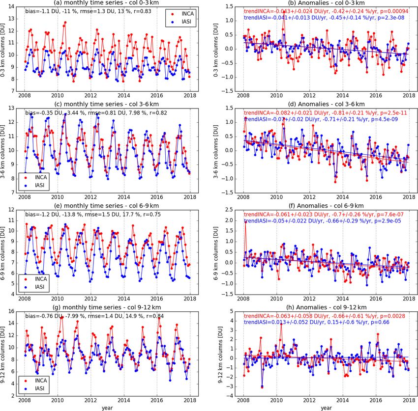
G. Dufour et al.: Recent ozone trends in the Chinese free troposphere                                                           16003

Figure 1. The northeastern Asian domain of the study. The following six subregions of interest are considered: Central East China (CEC;
28–42◦ N, 112–122◦ E), the Beijing–Tianjin–Hebei region (BTH; 37–41◦ N, 114–118◦ E), the Yangtze River Delta (YRD; 30–33◦ N, 118–
122◦ E), the Pearl River Delta (PRD; 21.5–24◦ N, 112–115.5◦ E), the Sichuan Basin (SCB; 28.5–31.5◦ N, 103.5–107◦ E), and the Korean
Peninsula–Japan region (KJ; 28–42◦ N, 122–145◦ E). Black circles show the rural-type surface stations and the red triangles the IAGOS
airports used in this study.

since September 2012, and one has been aboard the Metop-C             four et al., 2018), water vapour is fitted simultaneously with
platform since November 2018. The IASI instruments oper-              ozone to account for remaining interferences in the spectral
ate in the thermal infrared between 645 and 2760 cm−1 , with          windows used for the retrieval and to improve the retrieval in
an apodised resolution of 0.5 cm−1 . The field of view of the         the current version (3.0) of the product. From the retrieved
instrument is composed of a 2 × 2 matrix of pixels with a             profiles, different ozone partial columns can be calculated.
diameter at nadir of 12 km each. IASI scans the atmosphere            In this study, we consider the following four partial columns:
with a swath width of 2200 km and crosses the Equator at              the lowermost tropospheric (LMT) column from the surface
two fixed local solar times 09:30 LT (descending mode) and            to 3 km (named 0–3 km), the lower free tropospheric (LFT)
21:30 LT (ascending mode), allowing the monitoring of at-             column from 3 to 6 km (named 3–6 km), the upper free tropo-
mospheric composition twice a day at any location.                    spheric (UFT) column from 6 to 9 km (named 6–9 km), and
   Ozone profiles are retrieved from the IASI radiances us-           the upper tropospheric–lowermost stratospheric (UT-LMS)
ing the Karlsruhe Optimized and Precise Radiative transfer            column from 9 to 12 km (named 9–12 km). Note that only
Algorithm (KOPRA) radiative transfer model, its inversion             the morning overpasses of IASI are considered for this study
tool (KOPRAFIT), and an analytical altitude-dependent reg-            in order to remain in thermal conditions with a better sensi-
ularisation method, as described in Eremenko et al. (2008)            tivity to the lower troposphere. To cover a larger period, we
and Dufour et al. (2012, 2015). In order to avoid the poten-          also consider only IASI on Metop-A. Initial validation of the
tial impact of versioning of the auxiliary parameters (such           KOPRAFIT IASI ozone retrievals with ozonesondes and IA-
as temperature profile, clouds screening, etc.) on the ozone          GOS data is presented in Sect. 3.
retrieval (Van Damme et al., 2017), surface temperature and
temperature profiles are retrieved before the ozone retrieval.        2.2   Ozonesondes
A data screening procedure is applied to filter cloudy scenes
and to ensure the data quality (Eremenko et al., 2008; Dufour         Ozonesondes measure in situ vertical profiles of temperature,
et al., 2010, 2012). The a priori and the constraints are differ-     pressure, humidity, and ozone up to 30–35 km, with a vertical
ent, depending on the tropopause height, which is based on            resolution of ∼ 150 m for ozone. The ozonesondes data come
the 2 PV geopotential height product from the ECMWF (Eu-              mainly from the World Ozone and Ultraviolet Radiation Data
ropean Centre for Medium-Range Weather Forecasts). There              Centre (WOUDC) database (http://www.woudc.org/, last ac-
is one a priori and one constraint used for polar situations          cess: 19 October 2021), and the Southern Hemisphere Ad-
(i.e. tropopause < 10 km), one for midlatitude situations (i.e.       ditional Ozonesondes (SHADOZ) database (http://croc.gsfc.
tropopause within 10–14 km), and one for tropical situations          nasa.gov/shadoz/, last access: 19 October 2021). The sonde
(i.e. tropopause > 14 km). The a priori profiles are compiled         measurements use electrochemical concentration cell (ECC)
from the ozonesonde climatology of McPeters et al. (2007).            technique, relying on the oxidation of ozone with a potassium
Compared to the previous version of the ozone product (Du-            iodine (KI) solution (Komhyr et al., 1995), except the Ho-

https://doi.org/10.5194/acp-21-16001-2021                                            Atmos. Chem. Phys., 21, 16001–16025, 2021
16004                                                    G. Dufour et al.: Recent ozone trends in the Chinese free troposphere

henpeißenberg sondes, which use Brewer–Mast-type sondes.             2.5   OMI/MLS
Their accuracy for the ozone concentration measurement is
about ± 5 % (Deshler et al., 2008; Smit et al., 2007; Thomp-         Ozone Monitoring Instrument (OMI)/Microwave Limb
son et al., 2003). We use a database of ozonesonde measure-          Sounder (MLS) tropospheric column ozone is described by
ments from 2007 to 2012, including 24 stations in the mid-           Ziemke et al. (2019). The OMI/MLS ozone product rep-
latitudinal bands (30–60◦ ; both hemispheres), 13 stations in        resents monthly means for October 2004 to the present at
the tropical band (30◦ S–30◦ N) and 16 stations in the polar         1◦ × 1.25◦ resolution and a latitude range of 60◦ S–60◦ N.
bands (60–90◦ ; both hemispheres). A list of stations and re-        Tropospheric column ozone is determined by subtracting
lated information is provided in Table A1 (Appendix A).              co-located Microwave Limb Sounder (MLS) stratospheric
                                                                     column ozone from OMI total column ozone each day at
2.3   Surface measurements                                           each grid point. Tropopause pressure used to determine MLS
                                                                     stratospheric column ozone invoked the WMO (World Mete-
Observational data are issued from the China National En-            orological Organization) 2 K km−1 lapse rate definition from
vironmental Monitoring Centre (CNEMC) and archived at                National Centers for Environmental Prediction (NCEP) re-
https://quotsoft.net/air/ (last access: 3 May 2021). The data        analyses. OMI total ozone data are available from https:
set provides hourly data of criteria pollutants SO2 , O3 , NO2 ,     //ozonewatch.gsfc.nasa.gov/data/omi/ (last access: 22 April
CO, PM2.5 , and PM10 consolidated every day in near-real             2021). MLS ozone data can be obtained from https://mls.jpl.
time from May 2014. It has been used in several other studies        nasa.gov (last access: 19 October 2021). Estimated 1σ pre-
(e.g. Li et al., 2020; Yin et al., 2021). Only national-level data   cision for the OMI/MLS monthly mean gridded tropospheric
are available in this data set for about 1300 stations through-      columns of ozone (TCO) product is 1.3 DU.
out mainland China. In this study, we consider only the sta-
tions with more than 50 % of measurements available to en-           2.6   LMDZ-OR-INCA model
sure a good temporal coverage for the entire period (2014–
2017). In the domain shown in Fig. 1, this corresponds to 685        The LMDZ-OR-INCA global chemistry–aerosol–climate
stations. We classified the stations in the following different      model (hereafter referred to as INCA – INteraction with
types of environment: mountain, rural, suburban, urban, and          Chemistry and Aerosols) couples the LMDZ (Laboratoire
traffic, based on the approach developed by Flemming et al.          de Météorologie Dynamique; version 6) general circulation
(2005) for Europe. This method has the advantage of not re-          model (GCM; Hourdin et al., 2006), and the INCA (ver-
quiring any additional information other than the pollutant          sion 5) model online (Hauglustaine et al., 2004). The interac-
concentration. The relative amplitude of the diurnal cycle of        tion between the atmosphere and the land surface is ensured
O3 observations is used to evaluate the representative envi-         through the coupling of LMDZ with the ORCHIDEE (ORga-
ronment of the station, with the assumption that the larger          nizing Carbon and Hydrology In Dynamic Ecosystems; ver-
the amplitude of the diurnal ozone cycle is, the more the sta-       sion 9) dynamical vegetation model (Krinner et al., 2005). In
tion is in an urban environment. In our case, each station has       the present configuration, the model includes 39 hybrid ver-
been evaluated during the studied period (i.e. 2014–2017).           tical levels extending up to 70 km. The horizontal resolution
                                                                     is 1.25◦ in latitude and 2.5◦ in longitude. The primitive equa-
2.4   IAGOS data
                                                                     tions in the GCM are solved with a 3 min time step, large-
IAGOS (In-Service Aircraft for Global Observing System;              scale transport of tracers is carried out every 15 min, and
http://www.iagos.org, last access: 19 October 2021) is a Eu-         physical and chemical processes are calculated at a 30 min
ropean research infrastructure dedicated to measuring air            time interval. For a more detailed description and an ex-
composition (Petzold et al., 2016). The programme counts             tended evaluation of the GCM, we refer to Hourdin et al.
more than 62 000 flights between 1994 and 2021 with ozone            (2006). INCA initially included a state-of-the-art CH4 -NOx -
measurements. For the purpose of this study, we used all             CO-NMHC-O3 tropospheric photochemistry (Hauglustaine
profiles of ozone at any time of day available above north-          et al., 2004; Folberth et al., 2006). The tropospheric photo-
eastern China/Korean Peninsula between 2011 and 2017. On             chemistry and aerosols scheme used in this model version is
board the IAGOS commercial aircraft, ozone is measured               described through a total of 123 tracers, including 22 tracers
using dual-beam ultraviolet absorption monitor (time reso-           to represent aerosols. The model includes 234 homogeneous
lution of 4 s), with an accuracy and a precision estimated           chemical reactions, 43 photolytic reactions, and 30 hetero-
at about 2 nmol mol−1 and 2 %, respectively. Further infor-          geneous reactions. Please refer to Hauglustaine et al. (2004)
mation on the instrument is available in other articles (see         and Folberth et al. (2006) for the list of reactions included
Thouret et al., 1998; Nédélec et al., 2015). Long-term qual-         in the tropospheric chemistry scheme. The gas-phase ver-
ity and consistency have been assessed by Blot et al. (2021).        sion of the model has been extensively compared to ob-
                                                                     servations in the lower troposphere and in the upper tropo-
                                                                     sphere. For aerosols, the INCA model simulates the distribu-
                                                                     tion of aerosols with anthropogenic sources such as sulfates,

Atmos. Chem. Phys., 21, 16001–16025, 2021                                            https://doi.org/10.5194/acp-21-16001-2021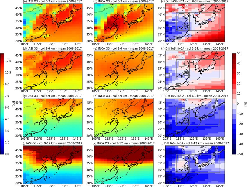
G. Dufour et al.: Recent ozone trends in the Chinese free troposphere                                                      16005

nitrates, black carbon, and particulate organic matter, as well   partial columns, and the Pearson correlation coefficient (R)
as natural aerosols such as sea salt and dust. Ammonia and        is larger than or equal to 0.79. Note that these results are
nitrates aerosols are considered as described by Hauglustaine     based on the comparison with ozonesonde profiles smoothed
et al. (2014). The model has been extended to include an in-      by the averaging kernels of the IASI retrieval. If we com-
teractive chemistry in the stratosphere and mesosphere (Ter-      pare with the raw sonde profiles without any smoothing, the
renoire et al., 2021). Chemical species and reactions specific    results are slightly degraded but remain good, with the nor-
to the middle atmosphere were added to the model. A total         malised biases within ± 5 %, the errors smaller than 30 %,
of 31 species were added to the standard chemical scheme,         and the correlations larger than 0.6. Version 3.0 of the O3
mostly belonging to the chlorine and bromine chemistry, and       IASI product reduces biases and increases the correlation
66 gas-phase reactions and 26 photolytic reactions.               with the ozonesondes measurements. The bias reduction is
   In this study, meteorological data from the European Cen-      the most effective in the upper troposphere.
tre for Medium-Range Weather Forecasts (ECMWF) ERA-                  In addition, we compared IASI ozone partial columns with
Interim reanalysis have been used to constrain the GCM me-        IAGOS ozone partial columns calculated from profiles mea-
teorology and allow a comparison with measurements. The           sured above Chinese and Korean Peninsula airports for the
relaxation of the GCM winds towards ECMWF meteorology             period 2011–2017. In this region, the IAGOS coverage was
is performed by applying, at each time step, a correction term    too sparse before this period. IAGOS profiles are filtered to
to the GCM u and v wind components, with a relaxation time        coincidence in space and time, with IASI pixels using the
of 2.5 h (Hauglustaine et al., 2004). The ECMWF fields are        same criteria as for the ozonesondes (1◦ around the station;
provided every 6 h and interpolated onto the LMDZ grid.           ± 6 h). The reference point for IAGOS to apply the coin-
   The historical global anthropogenic emissions are taken        cidence criteria is the middle of the profile. IAGOS pro-
from the Community Emissions Data System (CEDS) inven-            files with data missing above 500 hPa do not extend enough
tories (Hoesly et al., 2018) up to 2014. After 2014, the global   in altitude to be correctly compared to IASI observations,
anthropogenic emissions are based on Gidden et al. (2019).        and then they are not analysed. After these two filters, we
For China, the anthropogenic emission inventories are re-         count 213 IAGOS profiles for the time period 2011–2017.
placed the MEIC (Multi-resolution Emission Inventory for          These selected profiles are extended vertically between the
China) inventory (Zheng et al., 2018) available for the period    top (usually the cruise altitude of the aircraft) and 60 km,
2010–2017. The global biomass burning emissions are taken         with the a priori profiles used in the IASI retrieval. We apply
from van Marle et al. (2017) up to 2015 and from Gidden           the IASI averaging kernels to these extended IAGOS pro-
et al. (2019) after 2015. The ORCHIDEE vegetation model           files. The 500 hPa criterion to filter the IAGOS profiles is a
has been used to calculate the biogenic surface fluxes of iso-    compromise to have a reasonable number of profiles to com-
prene, terpenes, acetone, and methanol, as well as NO soil        pare with and to limit the contribution of a priori in the lower
emissions as described by Messina et al. (2016), offline.         tropospheric part of the smoothed profiles. Despite this, the
                                                                  resulting smoothed IAGOS profile may still be significantly
                                                                  affected by the a priori profile used to extend the raw IAGOS
3     Evaluation of the IASI O3 satellite product and             profile, especially when the cruise altitude of the profile is
      model simulations                                           low. Then, the comparison between IASI and IAGOS is the
                                                                  most meaningful below 500 hPa and for the partial columns
3.1    Validation of the IASI O3 product with                     representative of the lower free troposphere. We focus more
       ozonesondes and IAGOS                                      on the lower free tropospheric column (3–6 km) where the
                                                                  IASI retrievals are the most sensitive to ozone (Dufour et al.,
We present here a short validation of the version 3.0 of the      2012). Results are summarised in Table 1. The normalised
IASI O3 product developed at Laboratoire Interuniversitaire       mean bias and the normalised root mean square error esti-
des Systèmes Atmosphériques (LISA). A detailed validation         mate between IASI and IAGOS are −1.8 % and 17 %, re-
will be provided in a dedicated paper. The coincidence cri-       spectively when averaging kernels (AKs) are applied to IA-
teria used for the validation are 1◦ around the station, a time   GOS profiles (−5.6 % and 18 % without AKs applied) for
difference shorter than ± 6 h, and a minimum of 10 clear-sky      this column, which is in agreement with global ozonesonde
pixels matching these criteria. No correction factor has been     validation. The correlation is smaller (0.62) than the one with
applied on ozonesonde measurements as our main concern            the sondes (0.79). Statistics for the other columns are also re-
is the (lower) troposphere. The results of the comparison be-     ported in Table 1. The agreement is still good in terms of bias
tween IASI ozone retrievals and ozonesonde measurements           in the LMT (0–3 km) column but degrades in terms of cor-
are summarised in Table 1 for different partial columns in        relation. The temporal coincident criterion (± 6 h) combined
the troposphere. Normalised mean biases (NMB) for the dif-        with a non-negligible influence of the ozone diurnal cycle
ferent partial columns remain very small (< 2 %). The esti-       (Petetin et al., 2016) on the LMT (0–3 km) column might
mated errors given by the normalised root mean square error       explain the lower correlation for this column (0.45). In ad-
(NRMSE) range between 10 % and 20 %, depending on the             dition, the comparison made assuming a vertical profile at

https://doi.org/10.5194/acp-21-16001-2021                                       Atmos. Chem. Phys., 21, 16001–16025, 2021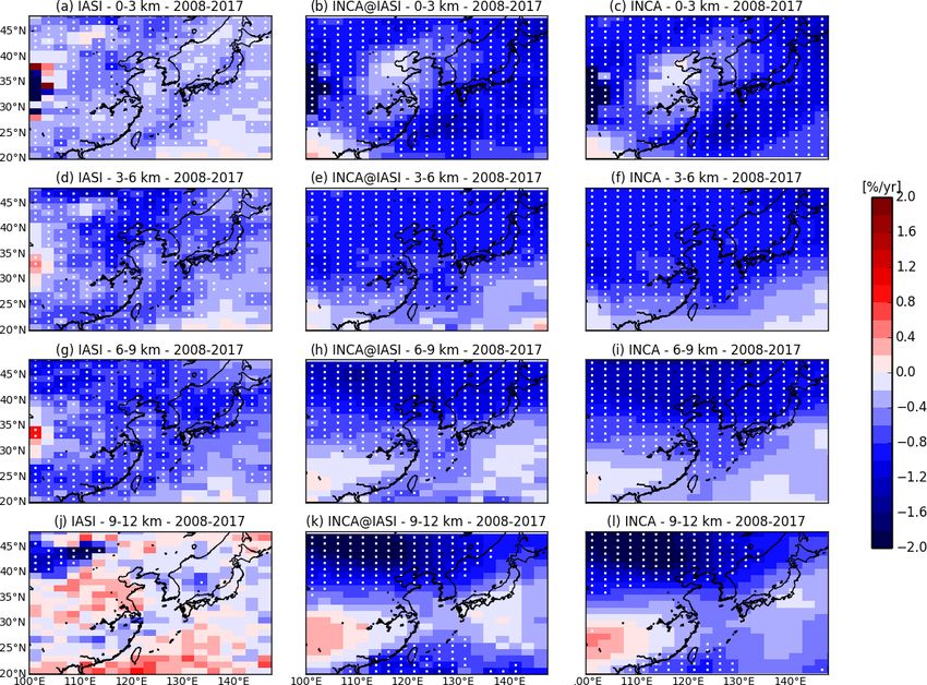
16006 G. Dufour et al.: Recent ozone trends in the Chinese free troposphere
Table 1. Statistics of the comparison of different O3 partial columns derived from IASI with O3 partial columns measured with ozonesondes
for 2007–2012 all the globe and with IAGOS for 2011–2017 for North China–Korean Peninsula. The normalised mean bias (NMB), the
normalised root mean square error (NRMSE), and the Pearson correlation coefficient (R) are provided.
Ozonesondes (2007–2012) IAGOS (2011–2017)
Columns NMB (%) NRMSE(%) R NMB (%) NRMSE (%) R
Surf–3 km −0.1 9.8 0.92 −2.5 14 0.45
3–6 km 0.5 14.8 0.79 −1.8 17 0.62
6–9 km 1.6 18.9 0.84 −2.5 25 0.59
9–12 km 1.3 18.6 0.92
Surf–6 km 0.2 12.3 0.84
Surf–12 km 0.9 13.7 0.89
Table 2. Comparison between the daily O3 concentrations simulated by the INCA model and the daily mean O3 concentrations measured
at the Chinese surface stations for 2014–2017. Due to the model resolution, only the stations classified as rural are used for the comparison.
For each region, the number of stations and the mean observed and simulated O3 concentrations are provided. The normalised mean bias
(NMB in percent) is calculated as the difference between the model concentration and the observed one, with the latter used as the reference.
The normalised root mean square error (NRMSE in percent) is calculated based on the daily averages, and the correlation coefficient (R)
corresponds to the temporal and the spatial correlation (the daily time series of each station are considered in its calculation without any
regional averaging).
Region No. of O3 stations O3 model NMB (%) NRMSE (%) R
stations (µg m−3 ) (µg m−3 )
China 125 66 74 12 50 0.42
CEC 41 70 72 3 48 0.49
BTH 4 77 67 −13 41 0.68
YRD 10 69 81 18 53 0.34
PRD 11 61 86 41 60 0.44
the latitude and longitude of the midpoint of a slant profile shows relatively good performances, especially in terms of
recorded during take-off and landing phases. The lowest part bias. However, the performances of the model in reproduc-
of the profile may be more influenced by urban areas near the ing the ozone concentration depend on the region. A good
airport and then be less reproduced by IASI due to its limited agreement is observed in the CEC region, with a bias of
sensitivity close to the surface. For the 6–9 km column, only 3 %, correlation of 0.49, and NRMSE of 48 %, respectively
50 profiles over 213 reach 300 hPa, and then the IAGOS pro- (Table 2). In the BTH region, north of the CEC, the mod-
files are largely mixed with the a priori profile used in the elled O3 concentrations are smaller than the observed ones
IASI retrieval. The evaluation of IASI using IAGOS is then (−13 %), but the correlation is higher (0.68). In the south of
difficult for the 6–9 km column with so few coincident obser- the CEC, the comparison in the YRD region remains satis-
vations. fying in terms of bias (18 %) but is degraded for the correla-
tion (0.34) and the NRMSE (53 %). In the coastal region of
3.2 Evaluation of the INCA simulations PRD, the available stations are within one model grid cell,
including land and sea. The coarse resolution of the model
likely limits its capability to reproduce correctly the O3 con-
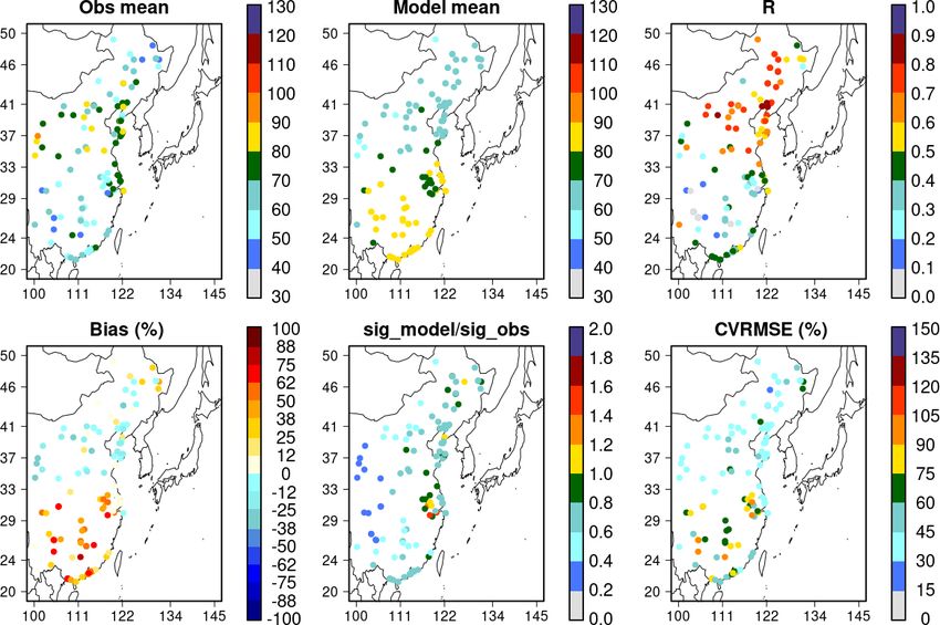
The model is evaluated using the Chinese surface network
centrations of the coastal stations: the model overestimates
described in Sect. 2.3. As the model resolution is coarse and
the surface measurements (41 %) with large NRMSE (60 %)
not representative of urban situations, we compare the model
and poor correlation (0.44). In the SCB, too few stations are
only with the rural-type stations. The daily O3 concentrations
available to provide statistics for the comparison. Figure A1
simulated by the model are compared to the daily averages
(Appendix A) shows the comparison station by station. Sim-
calculated from the hourly surface measurements provided
ilar results are shown with a very good agreement in the
by the Chinese surface network. The normalised mean bias
northern part of the domain; biases are within 10 %, corre-
between INCA and the surface stations is 12 % over the Chi-
lation is larger than 0.6, and NRMSE is smaller than 40 %.
nese domain considered, with INCA being larger. The corre-
In the southern part of the domain, the model has some dif-
lation and the normalised root mean square error (NRMSE)
ficulties in reproducing the observations, with biases ranging
are 0.42 % and 50 %, respectively. On average, the model
Atmos. Chem. Phys., 21, 16001–16025, 2021 https://doi.org/10.5194/acp-21-16001-2021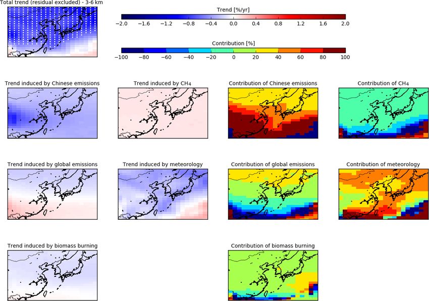
G. Dufour et al.: Recent ozone trends in the Chinese free troposphere 16007
from 30 % to 60 % for most of the stations and being larger the model to keep them independent of the observations and
for some stations. The correlation is limited, and the NRMSE a priori information used in the retrievals (see Sect. 4). Note
is larger than 50 %. In terms of trends, the 2014–2017 time that Barret et al. (2020) also discussed the interest in the con-
period is short to derive robust trends. When considering sideration of raw and smoothed data in satellite data proce-
observed and simulated trends at the surface with p values dures. Spatial distribution and spatial gradients of ozone are
smaller than 0.05, model and observations are rather consis- in good agreement for the four partial columns. On average,
tent, especially in regions where the model simulates the O3 the differences are smaller than 5 % for the 0–3 and 3–6 km
concentrations correctly (Fig. A2). The model tends to un- columns. The difference is larger for the upper columns – 6–
derestimate the positive trends compared to the observations. 9 and 9–12 km columns – with a mean negative difference
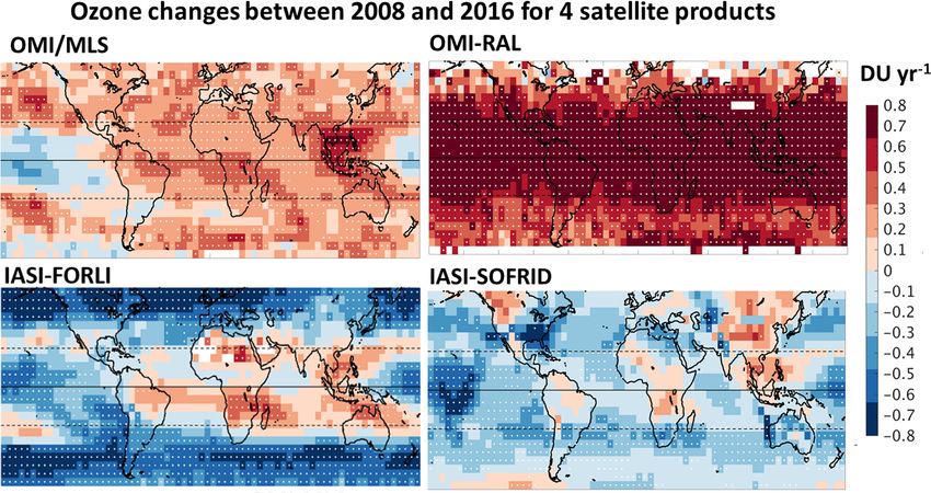
We use also IAGOS ozone profiles above Chinese and Ko- of about 7 % for both 6–9 and 9–12 km columns. For the 0–
rean Peninsula airports for the period 2011–2017 to evaluate 3 km partial column, it is worth noting that the IASI retrieval
the model above 950 hPa (Fig. 2). The selected IAGOS data is not highly sensitive to these altitudes and that the a pri-
correspond to the lowermost troposphere (950–700 hPa), the ori contribution is larger (Dufour et al., 2012). This is illus-
lower (700–470 hPa) and upper (470–300 hPa) free tropo- trated over China by IASI being systematically smaller than
sphere, and the UT-LMS (< 300 hPa) above the Chinese INCA without AK smoothing (−5 % to −25 %; Fig. A3a)
coast (east of 110◦ E and between 30 and 50◦ N) and South and an improved agreement (± 5 %) when applying the AKs
Korea. In order to assess more precisely the model’s ability to the model (Fig. 3a) and by larger differences over trop-
to reproduce the observed ozone behaviour, the IAGOS data ical maritime regions reduced when AKs are applied. The
are projected onto the model daily grid using the Interpol- agreement between IASI and INCA remains largely reason-
IAGOS software (Cohen et al., 2021a) and averaged every able, accounting for the observation and model uncertainties.
month. The subsequent product is hereafter called IAGOS- For the 3–6 km partial columns, where the IASI retrievals are
DM (Distributed onto the Model grid). We derive monthly the most sensitive, a very good agreement between IASI and
means from the INCA daily output by selecting the sampled INCA, within ± 10 %, is observed for a large part of the do-
grid cells. These monthly fields are called INCA-M (with M main (Figs. 3b and A3b). It is the partial columns for which
referring to the IAGOS mask). The two products IAGOS-DM the agreement is the best. For the upper columns (6–9 and
and INCA-M are, thus, consistent in space and time and can 9–12 km), IASI is almost systematically smaller than INCA
be compared together. It is important to note that the regional over the domain (Figs. 3c and d and A3c and d). IASI is al-
averages calculated here do not account for the tropopause ways smaller than INCA over most of China, despite what
altitude, in contrast to Cohen et al. (2021a). Last, as in Co- the partial columns considered. IASI is mainly larger than
hen et al. (2018), the statistical representativeness of the ob- INCA in the lower troposphere and smaller in the upper tro-
servations is enhanced by filtering out the regional monthly posphere elsewhere. In the desert northwestern part of the
means either with fewer than 300 measurement points or domain, even if the emissivity is included in the IASI re-
fewer than 7 d separating the first and the last measurements. trievals, the quality of the retrievals can be affected and confi-
A very good agreement is observed between the INCA model dence in the data reduced. This region is then not considered
and the IAGOS observations, with small biases ranging from here. The retrieval in the tropical-type air masses have been
1.6 % in the lower free troposphere to 12 % in the lowermost shown to reinforce the natural S shape of the ozone profiles,
troposphere. The INCA and IAGOS time series are well cor- leading to some overestimations of ozone in the lower tropo-
related with correlation coefficients equal to or larger than sphere and an underestimation in upper troposphere (Dufour
0.76. Looking in detail, the time series shows that the model et al., 2012). This likely explains the positive and negative
tends to underestimate O3 in the lowermost troposphere and differences with the model in the southeastern part of the do-
to underestimate the largest O3 values in the lower and the main (Fig. A3). Globally, the differences between IASI and
upper free troposphere. INCA are the smallest over Central East China (CEC). Fig-
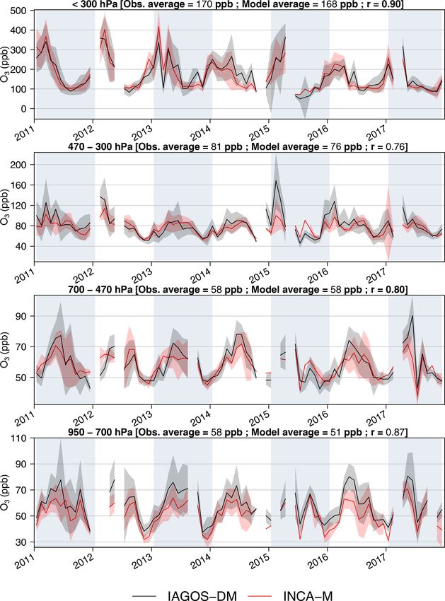
ure 4 shows the IASI and INCA monthly time series of the
3.3 Comparison between IASI O3 product and INCA different O3 partial columns between 2008 and 2017 for this
simulation in northeastern Asia region. The INCA time series are the series from which the
trends are derived (Sect. 4), and then do not included any
We compare IASI and INCA O3 partial columns over the smoothing from the IASI AKs. The correlation between the
East Asia domain (100–145◦ E, 20–48◦ N) averaged over the IASI and INCA time series is good as it is larger than 0.8,
2008–2017 period. To properly compare IASI and INCA, the except for the 6–9 km column (0.75). The high correlation
model is smoothed by IASI averaging kernels (AKs; Fig. 3). is partly driven by the seasonal cycle, but the correlation
The comparison without any smoothing of the model is also remains quite high for deseasonalised (anomalies) series –
shown in the Appendix (Fig. A3). This latter comparison is 0.65, 0.63, and 0.68 for 0–3, 3–6 and 9–12 km columns, re-
also interesting for the determination of the deviation of the spectively – except for the 6–9 km column (0.44). Biases
observations compared to the native model resolution as the ranging from 8 % to 14 %, with INCA being larger, are ob-
simulated trends are calculated without applying the AKs to served between IASI and INCA for the 0–3, 6–9, and 9–
https://doi.org/10.5194/acp-21-16001-2021 Atmos. Chem. Phys., 21, 16001–16025, 2021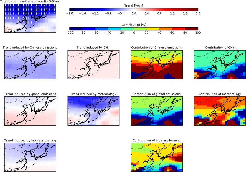
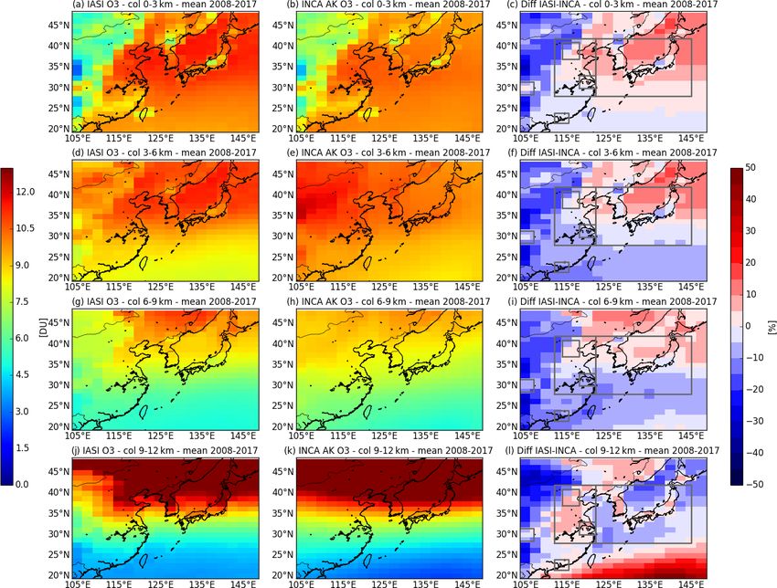
16008                                                      G. Dufour et al.: Recent ozone trends in the Chinese free troposphere

Figure 2. Ozone monthly mean values derived in four altitude domains representing the LMT, LFT, UFT, and UT-LMS (from bottom to
top) from the gridded IAGOS data set (solid black line) and the simulation output (solid red line) over northeastern Asia, with respect to the
IAGOS mask. The uncertainties are defined by the regional average of the standard deviations calculated for each grid cell. For each altitude
domain, the yearly O3 concentration derived from the mean seasonal cycle is indicated above the corresponding graphic for both data sets,
with the Pearson correlation coefficient comparing the two monthly time series.

12 km columns, respectively. The highest values are larger                  In the following, after presenting the trend analysis glob-
with INCA for the 0–3 and 9–12 km columns, and the lowest                ally over the Asian domain for the different partial columns,
values are larger for the 6–9 km columns (Fig. 4). A smaller             the discussion will focus more on the 3–6 km partial column
bias (−3.4 % on average) better balanced between small and               where IASI and INCA agree well. The CEC region will also
large values is observed for the 3–6 km column (Fig. 4b). The            be prioritised in the discussion, as the model and observation
seasonal cycle observed with IASI is reasonably reproduced               operate better, and they are in rather good agreement in this
by the model for the different partial columns, with a better            region. Some other highly populated and polluted regions,
agreement in the 3–6 and 9–12 km columns. However, the                   such as the Sichuan Basin (SCB) and the Pearl River Delta
summer drops observed with IASI in the lower troposphere                 (PRD), will be also discussed, keeping in mind the largest
(0–3 and 3–6 km) are not systematically reproduced by the                differences between model and observations. As we show
model, and the summer maximum is shifted for the 6–9 km                  here, comparisons between IASI and INCA are satisfying
column.                                                                  with and without the application of AKs to the model. For

Atmos. Chem. Phys., 21, 16001–16025, 2021                                                  https://doi.org/10.5194/acp-21-16001-2021
G. Dufour et al.: Recent ozone trends in the Chinese free troposphere                                                               16009

Figure 3. Mean O3 partial columns for 2008–2017 observed with IASI (a, d, g, and j), simulated by INCA (b, e, h, and k), and their
differences (c, f, i, and l). The INCA ozone profiles are smoothed by each individual IASI AKs. The following different partial columns are
considered: the lowermost tropospheric columns from the surface to 3 km altitude (named 0–3 km), the lower free tropospheric columns from
3 to 6 km altitude (named 3–6 km), the upper free tropospheric column from 6 to 9 km (named 6–9 km), and the upper tropospheric column
from 9 to 12 km (named 9–12 km).

the trend analysis, we will consider the model without AKs              units per year or in percent per year. As an ordinary linear re-
applied to avoid introducing retrieval a priori information in          gression is used for trend calculation, the trends uncertainties
the model and have a model fully independent of the obser-              are calculated as the t test value multiplied with the standard
vations. This will allow us to exploit the sensitivity tests con-       error of the trends, which correspond to the 95 % confidence
ducted with the model to determine the processes that drive             interval. The p values are also calculated and reported when
the trends.                                                             possible. An example is given in Fig. 4 for the CEC, with
                                                                        monthly time series on the left and anomalies on the right.
                                                                           Figure 5 presents the 2008–2017 O3 trends derived for dif-
4   O3 trends: satellite and model comparison                           ferent partial columns over the Asian domain using IASI and
                                                                        INCA. Trends derived from IASI are negative, with p < 0.05
To derive the trends, we first calculate the monthly time se-           for most of the domain and the different partial columns,
ries either at the INCA resolution – gridding IASI at this              except in the upper troposphere (9–12 km column). They
resolution – or averaging the model or observation partial              range between −0.2 and −0.6 % yr−1 for the 0–3 km col-
columns over the regions reported in Fig. 1. The monthly                umn and between −0.4 and −1 % yr−1 for the 3–6 and 6–
mean ozone values are used to calculate a mean 2008–2017                9 km columns. The trends derived from the model are rather
seasonal cycle. This cycle is then used to deseasonalise the            uniform over the domain for the 0–3 and 3–6 km columns,
monthly mean time series by calculating the anomalies. The              which are smaller than −1 % yr−1 , except in the CEC region
linear trend is then calculated based on the monthly anoma-             where the trends tend to zero in the lowermost troposphere
lies and a linear regression. It is provided either in Dobson

https://doi.org/10.5194/acp-21-16001-2021                                              Atmos. Chem. Phys., 21, 16001–16025, 2021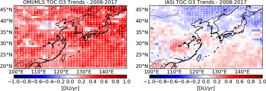
16010                                                   G. Dufour et al.: Recent ozone trends in the Chinese free troposphere

Figure 4. IASI and INCA monthly time series (a, c, e, and g) and anomalies (b, d, f, and h) for the 0–3, 3–6, 6–9, and 9–12 km O3 partial
columns over the CEC region for 2008–2017. Biases, RMSE, and Pearson correlation coefficient between the IASI and INCA monthly time
series are provided, as well as the trends, uncertainties, and associated p values calculated from the anomalies time series.

(0–3 km). It is worth noting that the model shows positive             The trends derived from the model resampled to match IASI
trends at the surface level in this region (not shown), which          observations are reported on Fig. 5. The resampling only
is in agreement with surface measurement studies (e.g. Li              slightly changes the trends derived from the model. In the
et al., 2020). A residual positive trend is observed up to 1 km        following, we consider the model without matching the IASI
altitude in the model and becomes negative higher up (not              sampling.
shown). The trends in the mid–upper troposphere (6–9 km                   Table 3 summarises the O3 trends derived from IASI and
and 9–12 km columns) are mainly negative (p < 0.05) in the             INCA for different partial columns and for the different re-
north to 30◦ N latitude and can be more variable in the sub-           gions reported in Fig. 1. We choose the most populated
tropics (Fig. 5). To evaluate the impact of the IASI sam-              Chinese areas where significant pollutant reductions have
pling (representative of clear-sky conditions), we calculate           occurred since 2013 (Zheng et al., 2018), such as CEC –
the model monthly mean, including the model grid cells on              including BTH and YRD – and PRD and SCB. We also
the days when IASI observations are available in these cells.          consider the KJ region as a region influenced by the pol-

Atmos. Chem. Phys., 21, 16001–16025, 2021                                               https://doi.org/10.5194/acp-21-16001-2021
G. Dufour et al.: Recent ozone trends in the Chinese free troposphere                                                                  16011

Figure 5. Trends calculated in percent per year at the 2.5◦ × 1.25◦ resolution for the 0–3, 3–6, 6–9, and 9–12 km O3 partial columns. Panels
(a, e, i, and m) show the trends derived from IASI, panels (b, f, j, and n) show the trends derived from INCA sampled over the IASI pixels,
panels (c, g, k, and o) show the trends derived from INCA with its native daily resolution, and panels (d, h, l, and p) show the trends derived
from the INCA reference simulation minus the MET simulation (see the text and Table 4 for details). White crosses are displayed when
p values are smaller than 0.05.

lution export from China. We made the trend values bold                   the model and the observations are less reliable for different
in the table when both IASI and INCA have trends with                     reasons explained in Sect. 3. This leads to a poor agreement
p < 0.05 and when the trends agree within 40 % between the                of the derived trends and a lack of reliability of the trends
model and the observations. The trend values correspond-                  for these two regions (large uncertainties in the trend val-
ing to p < 0.05 and a poorer agreement are italicised. The                ues; Table 3). For the BTH and YRD, included in the CEC,
CEC region shows the best agreement between the trends                    and for the KJ, the trends calculated from the observations
derived from IASI and INCA for all the columns, except the                and the model are in good agreement for the 3–6 and 6–9 km
upper tropospheric columns (9–12 km). The anomalies and                   columns, with p < 0.01.
calculated linear trends are shown in detail on Fig. 4b, d, f
and h. For this region, where both the observations and the
model are the most reliable, trends are in very good agree-               5     Discussion
ment (< 15 %) for the 0–3, 3–6, and 6–9 km columns. Trends
derived from IASI for the UT-LMS columns (9–12 km) are                    5.1    Evaluation of the processes contributing to the
very small, with large p values for all the regions (Table 3). It                trends
is then difficult to compare and conclude for the upper tropo-
spheric columns as the trends calculated from the model are               In this work focused on China and the period of 2008–2017,
mainly negative, with p < 0.05. For the PRD and the SCB,                  both IASI observations and INCA simulations show negative
                                                                          O3 trends of similar magnitude in the lower (3–6 km) and up-

https://doi.org/10.5194/acp-21-16001-2021                                                 Atmos. Chem. Phys., 21, 16001–16025, 2021
16012 G. Dufour et al.: Recent ozone trends in the Chinese free troposphere
Table 3. Calculated trends in Dobson units per year from IASI observations and INCA simulations for the different regions of Fig. 1 and
the 0–3, 3–6, 6–9, and 9–12 km partial columns. The associated p value is indicated for each trend. The trend values are shown in bold font
when both IASI and INCA trends have associated p < 0.05 and are within 40 % agreement. The trend values are shown with italics when
both IASI and INCA trends have associated p < 0.05 but with differences larger than 40 %.
0–3 km 3–6 km 6–9 km 9–12 km
IASI INCA IASI INCA IASI INCA IASI INCA
CEC −0.04 ± 0.01 −0.04 ± 0.02 −0.07 ± 0.02 −0.08 ± 0.02 −0.05 ± 0.02 −0.06 ± 0.02 0.01 ± 0.05 −0.06 ± 0.06
(p < 0.01) (p < 0.01) (p < 0.01) (p < 0.01) (p < 0.01) (p < 0.01) (p = 0.66) (p < 0.01)
BTH −0.05 ± 0.01 −0.02 ± 0.01 −0.09 ± 0.02 −0.09 ± 0.01 −0.06 ± 0.03 −0.09 ± 0.04 0.02 ± 0.07 −0.11 ± 0.10
(p < 0.01) (p = 0.16) (p < 0.01) (p < 0.01) (p < 0.01) (p < 0.01) (p = 0.61) (p < 0.01)
YRD −0.03 ± 0.02 −0.06 ± 0.04 −0.05 ± 0.03 −0.08 ± 0.03 −0.05 ± 0.03 −0.05 ± 0.03 −0.009 ± 0.06 −0.02 ± 0.05
(p = 0.04) (p < 0.01) (p < 0.01) (p < 0.01) (p < 0.01) (p < 0.01) (p = 0.54) (p = 0.05)
KJ −0.03 ± 0.01 −0.09 ± 0.03 −0.06 ± 0.02 −0.08 ± 0.02 −0.05 ± 0.02 −0.06 ± 0.03 −0.01 ± 0.05 −0.05 ± 0.06
(p < 0.01) (p < 0.01) (p < 0.01) (p < 0.01) (p < 0.01) (p < 0.01) (p = 0.49) (p = 0.03)
PRD −0.04 ± 0.02 −0.05 ± 0.06 −0.06 ± 0.02 −0.03 ± 0.04 −0.04 ± 0.02 −0.03 ± 0.04 0.009 ± 0.03 −0.04 ± 0.03
(p < 0.01) (p = 0.09) (p < 0.01) (p = 0.22) (p < 0.01) (p = 0.15) (p = 0.67) (p = 0.02)
SCB −0.007 ± 0.01 −0.02 ± 0.006 −0.02 ± 0.02 −0.08 ± 0.03 −0.02 ± 0.02 −0.02 ± 0.03 0 ± 0.04 0.02 ± 0.03
(p = 0.07) (p < 0.01) (p < 0.01) (p < 0.01) (p = 0.05) (p = 0.24) (p = 0.89) (p = 0.23)
Table 4. Description of the different simulations done with the INCA model and the trends calculation. Note that, for all the simulations, the
biogenic emissions are constant over the period.
Simulationsa Trend calculationb
SR = Reference Total Trend(SR)
SC = no China variations China Trend(SR) – trend(SC)
SG = no China and no global variations Global Trend(SC) – trend(SG)
SB = no China and no global and no biomass burning variations BBg Trend(SG) – trend(SB)
S4 = no China and no global and no biomass burning and no methane variations CH4 Trend(SB) – trend(S4)
SM = no China and no global and no biomass burning and no methane and no meteo variations MET Trend(S4)
a All the simulations are corrected from residual O variations (see text). b The contribution of each process to the trend is calculated by dividing the corresponding trend by
3
the total trend (TT).
per (6–9 km) free troposphere in large parts of China and its are maintained at their 2007 values. Since the INCA model
downwind region. Dufour et al. (2018) suggest that negative is a GCM, this method reduces considerably the interan-
O3 trends derived from IASI in the lower troposphere over nual variability associated with meteorology. However, the
the North China Plain for a slightly shorter time period can meteorology is not identical from 1 year to another in the
be explained for almost half by NOx emissions reduction that GCM. This leads to a residual trend as shown in Fig. B1
has been occurring in China since 2013. They argue the neg- (Appendix B) for the different partial columns. This residual
ative impact on the trend of these reductions compared to the trend is mainly negative and small. To remove this residual
positive one at the surface is due to changes in the chemical trend from the model results, we subtract the meteorologi-
regime with the altitude. To go further on this and quantify cal variability (MET) simulation to the other simulations day
the processes contributing to the O3 trends, we performed by day and grid cell by grid cell. The trends derived from
several simulations with the INCA model. The objective is the initial simulation corrected from the residual ozone vari-
to remove, one by one, the interannual variability and trend ations are slightly increased compared to the trends derived
induced by the different processes (emissions and meteorol- from the initial simulation, but they remain fully consistent,
ogy). The different simulations are summarised in Table 4. especially when p < 0.05. Then, we calculate the trend and
First, anthropogenic emissions in China are kept constant to contribution of each process as described in Table 4.
their 2007 values during the 2008–2017 period. Then, in ad- The contribution of the different processes is shown in
dition, the global anthropogenic emissions for the rest of the Fig. 6 for the 3–6 km columns and in Fig. B2 for the 6–
world are kept constant to their 2007 values, the biomass 9 km columns. We focus on these two columns as they cor-
burning emissions, and then the methane concentrations. Fi- respond to the tropospheric regions where IASI is the most
nally, winds used for nudging and sea surface temperatures sensitive and then where agreement with the model is the
Atmos. Chem. Phys., 21, 16001–16025, 2021 https://doi.org/10.5194/acp-21-16001-2021G. Dufour et al.: Recent ozone trends in the Chinese free troposphere 16013
Figure 6. Trends and contributions of the meteorological variability, the Chinese anthropogenic emissions, the global anthropogenic emis-
sions, the global biomass burning emissions, and the CH4 to the trends calculated for the 3–6 km (see Table 4 for details on the simulations).
Table 5. Contributions (in percent) of the meteorological variability (MET), the Chinese anthropogenic emissions (China), the global an-
thropogenic emissions (Global), the global biomass burning emissions (BBg), and the CH4 to the trends calculated for the 3–6 and 6–9 km
partial columns for each individual region in Fig. 1.
3–6 km partial column 6–9 km partial column
MET CH4 BBg Global China MET CH4 BBg Global China
CEC 34.3 −15.2 13.4 7.4 60.1 50.0 −14.9 18.1 −5.4 52.2
BTH 37.8 −14.5 14.7 21.9 40.1 55.4 −11.4 17.0 4.1 34.8
YRD 34.2 −15.9 13.1 −2.5 71.0 42.0 −17.4 14.7 −18.7 79.5
KJ 37.9 −15.2 18.6 11.8 46.9 46.1 −15.6 30.2 −3.4 42.7
best. We also focus mainly on China where the p values of to the other processes (emissions and meteorology). In the
the total trend are smaller than 0.05. In the lower free tro- upper free troposphere, meteorology and Chinese emissions
posphere, the main contributions to the trends are the local also dominate the contributions. Biomass burning emissions
Chinese emissions and the meteorology, with contributions also play a more important role in explaining the trend in
larger than 20 %. The other tested variables (global emis- the North China Plain between the Beijing region and the
sions, biomass burning emissions, and methane) contribute to Yangtze River. In the south of the domain, where the robust-
the trends within 20 % over mainland China, with a negative ness of the trends might be discussed as p values are larger
contribution of methane for the entire domain. This means than 0.05, strong compensations seem to operate between the
that the increase in methane concentrations and then the asso- contributions of the different processes, leading to a less ro-
ciated ozone production counteracts the ozone reduction due bust assessment of their respective contributions. The differ-
https://doi.org/10.5194/acp-21-16001-2021 Atmos. Chem. Phys., 21, 16001–16025, 202116014 G. Dufour et al.: Recent ozone trends in the Chinese free troposphere
ent contributions for the regions where the model and the ob- period, and to the starting and ending point of the time se-
servations are the most reliable are detailed in Table 5. Chi- ries. Due to the availability of the satellite measurements and
nese emissions contribute to 60 % in the main source region, the simulated period with the model, it was not possible to
the CEC, with variations inside the regions for the 3–6 km extend the time period further. We tested the impact of the
column; the Chinese emissions contribute to 40 % in BTH starting and ending point of the time series by removing 1
and more than 70 % in YRD. The Chinese contribution to and 2 years at the beginning and at the end of the period. The
the trends in the export region (KJ) remains high, with 47 % trends derived from IASI and INCA for the 3–6 km column
contribution. The meteorological contribution ranges from in the CEC for the different periods are summarised in Ta-
34 % to 38 %. Methane and biomass burning emissions con- ble B1 (Appendix B). They remain consistent with the trend
tributions are rather stable over the different regions around derived for 2008–2017, respectively for IASI and INCA, and
−15 % and +14 %, respectively, with the biomass burning are within its confidence interval. These results corroborate
contribution being slightly higher in the export region (19 % the consistency between the modelled and observed trends
for KJ). Surprisingly, the global emissions contribute the and their robustness. However, it is worth noting that the cal-
most to the trends in the highly polluted region of the BTH culated trends seem more sensitive to the end of the period,
(22 %). For the 6–9 km column, the meteorological contribu- corresponding to a strong El Niño period, than to the begin-
tion to the trends increases (about 50 % or larger) as the Chi- ning of the period. Removing the last 2 years of the period
nese emissions contribution decreases. The biomass burning leads to a decrease in the IASI trend and to an increase in
contribution is globally larger, especially in the export region the INCA trend. This apparent inconsistency, which should
where it reaches 30 %. The global anthropogenic emissions be evaluated when longer simulations with consistent emis-
contribution remains small in absolute value, except in the sions and longer observation time series will be available,
YRD region where it becomes negative and reaches −20 %. stresses the difficulty of working with short-term trends and
The prevailing contribution of Chinese emissions changes in the need for caution to prevent overinterpreting the results. It
the negative O3 trends in the lower and upper free tropo- is worth noting that using the Theil–Sen estimator to calcu-
sphere seems to confirm the previous outcomes of Dufour late the trends changes only slightly the trends.
et al. (2018).
Discrepancies between different satellite sounders and
5.2 Limitation of the study products
The results presented in our study are not fully in line with The TOAR points toward the following major discrepancy
the recent TOAR (Gaudel et al., 2018) and related works between the different satellite ozone products available for
(Cooper et al., 2020; Gaudel et al., 2020), which state a the report: the OMI UV sounder showing mainly positive
general increase in tropospheric ozone during the last few trends over 2008–2016 and the IASI IR sounder showing
decades. If negative trends are observed at the surface in de- mainly negative trends over the same period (Fig. B3; Ap-
veloped countries, for example, in summer, positive trends pendix B). Over northeastern Asia, the discrepancy in the
for the free troposphere are reported using mainly IAGOS as sign of the trend calculated from the different satellite prod-
a reference (Cooper et al., 2020). It is worth noting that this ucts is contrasted more. The OMI/MLS and OMI-RAL prod-
study brings another angle to the question of ozone changes ucts still show positive trends as all over the globe. The
with time over China than previously discussed during Phase IASI-SOFRID (SOftware for a Fast Retrieval of IASI Data)
I of TOAR. In the TOAR effort, our IASI product was used product shows positive trends all over China, and the IASI-
to describe the seasonal variability in ozone for the time pe- FORLI (Fast Optimal Retrieval on Layers for IASI) prod-
riod of 2010–2014 over China. However, this product was uct positive trends only in the southeastern part of China.
not used to assess ozone trends. Compared to the other IASI The IASI O3 product used in this study was not included
products, our product is more sensitive to the lower part of in the comparison as it is not a global product. It is worth
the troposphere (see Table 2 in Gaudel et al., 2018). We hope noting that, for the TOAR, the tropospheric columns de-
this study can bring more information to fuel the discus- rived from the different satellite products were not based
sion on the discrepancies between the UV and IR techniques. on the same tropopause height definition, and each product
Even if our study seems to show consistent trends derived by was considered with its native sampling. This might con-
IASI and the model in the free troposphere, we stress, in this tribute partly to the differences between the trends, in addi-
subsection, vigilant points for the interpretation of the results. tion to the fundamental differences in the measurement tech-
niques (UV and IR) and the retrieval algorithms used. Possi-
Length of the period ble drifts over the time have not been systematically studied
in the TOAR. Some individual studies exist, but once again,
In this study, we derived trends over a limited 10-year period. they do not allow one to draw conclusions concerning the
Calculating short-term trends leads to an increased sensitiv- role of the drifts in the trend discrepancies. Indeed, Boynard
ity to the inter- and intra-annual variations, the length of the et al. (2018) noticed a significant negative drift in the North-
Atmos. Chem. Phys., 21, 16001–16025, 2021 https://doi.org/10.5194/acp-21-16001-2021You can also read