Generator Fleet Characteristics Model - NIST Technical Note NIST TN 2246 - Cheyney O'Fallon Avi Gopstein - TSAPPS at NIST
←
→
Page content transcription
If your browser does not render page correctly, please read the page content below
NIST Technical Note
                            NIST TN 2246

Generator Fleet Characteristics Model

                                            Cheyney O’Fallon
                                                Avi Gopstein

                 This publication is available free of charge from:
                           https://doi.org/10.6028/NIST.TN.2246
NIST Technical Note
NIST TN 2246
Generator Fleet Characteristics Model
Cheyney O’Fallon
Avi Gopstein
Smart Grid Group
Communications Technology Laboratory
This publication is available free of charge from:
https://doi.org/10.6028/NIST.TN.2246
February 2023
U.S. Department of Commerce
Gina M. Raimondo, Secretary
National Institute of Standards and Technology
Laurie E. Locascio, NIST Director and Under Secretary of Commerce for Standards and TechnologyNIST TN 2246 February 2023 Certain commercial entities, equipment, or materials may be identifed in this document in order to describe an experimental procedure or concept adequately. Such identifcation is not intended to imply recommendation or endorsement by the National Institute of Standards and Technology, nor is it intended to imply that the entities, materials, or equipment are necessarily the best available for the purpose. NIST Technical Series Policies Copyright, Fair Use, and Licensing Statements NIST Technical Series Publication Identifer Syntax Publication History Approved by the NIST Editorial Review Board on 2023-02-01 How to cite this NIST Technical Series Publication: O’Fallon C, Gopstein A (2023) Generator Fleet Characteristics Model. (National Institute of Standards and Technology, Gaithersburg, MD), NIST TN 2246. https://doi.org/10.6028/NIST.TN.2246 NIST Author ORCID iDs Cheyney O’Fallon: 0000-0002-5931-4173 Avi Gopstein: 0000-0002-5654-669X Contact Information cheyney.ofallon@nist.gov
NIST TN 2246
February 2023

Abstract

This manuscript presents the Generator Fleet Characteristics Model (GFCM), a general purpose
tool for the analysis of power system operations, economics, and resilience. The GFCM is a
collection of MATLAB functions that use publicly available data with national coverage to produce
year-long (8760 hour) analyses of the electric grid at the balancing authority level. As the name
implies, the GFCM builds up a series of snapshots of electric grid conditions and outcomes using
the economics of the generator feet as a starting point for understanding system complexity and
dynamics. While the synchronous inertia application we present here uses the GFCM to build a
detailed picture of the present state of electric grid operations and market outcomes, the model is
designed to facilitate counterfactual study through the comparison of model outputs by an analyst
that systematically varies inputs. The GFCM forms a modeling framework intended to aide in the
formulation of “what if” questions regarding how the grid might operate under changing ambient
conditions while harnessing evolving technologies.

Keywords

Economics; Electricity; Generator Fleet; Infrastructure; Interoperability; Operations; Power Sys-
tems; Resilience; Smart Grid; Synchronous Inertia.

                                                 i
NIST TN 2246
February 2023
Table of Contents
1. Introduction . . . . . . . . . . . . . . . . . . . . . . . . . . . . . . . . . . . . . . . . . . . . . 1
1.1. Changing Composition of Useful Phenomena . . . . . . . . . . . . . . . . . . . . . . 2
1.2. A Simple Model of Generating Fleet Characteristics . . . . . . . . . . . . . . . . . . 3
2. Model . . . . . . . . . . . . . . . . . . . . . . . . . . . . . . . . . . . . . . . . . . . . . . . . . 4
2.1. Model Purpose . . . . . . . . . . . . . . . . . . . . . . . . . . . . . . . . . . . . . . . . 5
2.2. Primary Data Inputs . . . . . . . . . . . . . . . . . . . . . . . . . . . . . . . . . . . . . 5
2.2.1. Static EIA Data . . . . . . . . . . . . . . . . . . . . . . . . . . . . . . . . . . . 6
2.2.2. EIA API Data . . . . . . . . . . . . . . . . . . . . . . . . . . . . . . . . . . . . 6
2.2.3. Scenario Specifcation . . . . . . . . . . . . . . . . . . . . . . . . . . . . . . . 7
2.3. Auxiliary Data Inputs . . . . . . . . . . . . . . . . . . . . . . . . . . . . . . . . . . . . 7
2.3.1. Inertia from Motor Loads . . . . . . . . . . . . . . . . . . . . . . . . . . . . . 8
2.3.2. Inertia from Private Use Networks . . . . . . . . . . . . . . . . . . . . . . . . 8
2.3.3. Weather Conditions . . . . . . . . . . . . . . . . . . . . . . . . . . . . . . . . . 8
2.4. Process Modules . . . . . . . . . . . . . . . . . . . . . . . . . . . . . . . . . . . . . . . 9
2.4.1. Fleet Selection . . . . . . . . . . . . . . . . . . . . . . . . . . . . . . . . . . . . 9
2.4.2. Marginal Cost Determination . . . . . . . . . . . . . . . . . . . . . . . . . . . 9
2.4.3. Generator Allocation . . . . . . . . . . . . . . . . . . . . . . . . . . . . . . . . 10
2.4.4. Market Snapshot . . . . . . . . . . . . . . . . . . . . . . . . . . . . . . . . . . 11
2.4.5. Auxiliary Sources of Inertial Contributions . . . . . . . . . . . . . . . . . . . . 12
2.4.6. Function Descriptions . . . . . . . . . . . . . . . . . . . . . . . . . . . . . . . . 13
2.4.6.1. gfcm v1 scenario specifer.m . . . . . . . . . . . . . . . . . . . . . . 13
2.4.6.2. gfcm v1 scenario main.m . . . . . . . . . . . . . . . . . . . . . . . . 13
2.4.6.3. gfcm v1 scenario snapshot.m . . . . . . . . . . . . . . . . . . . . . 13
2.4.6.4. gfcm v1 validation.m . . . . . . . . . . . . . . . . . . . . . . . . . . 13
2.4.6.5. gfcm v1 event focus graphics.m . . . . . . . . . . . . . . . . . . . . 14
2.4.6.6. gfcm v1 dir parent.m . . . . . . . . . . . . . . . . . . . . . . . . . . 14
2.4.6.7. gfcm v1 eia api call.m . . . . . . . . . . . . . . . . . . . . . . . . . 14
2.4.6.8. gfcm v1 api url constructor.m . . . . . . . . . . . . . . . . . . . . . 14
2.4.6.9. gfcm v1 api v2 data handler.m . . . . . . . . . . . . . . . . . . . . 14
2.4.6.10. gfcm v1 recursive.m . . . . . . . . . . . . . . . . . . . . . . . . . . . 14
iiNIST TN 2246
February 2023
2.4.6.11. gfcm v1 eia api key.m . . . . . . . . . . . . . . . . . . . . . . . . . . 15
2.5. Model Outputs . . . . . . . . . . . . . . . . . . . . . . . . . . . . . . . . . . . . . . . . 15
2.6. Model Validation . . . . . . . . . . . . . . . . . . . . . . . . . . . . . . . . . . . . . . . 20
3. Tutorial . . . . . . . . . . . . . . . . . . . . . . . . . . . . . . . . . . . . . . . . . . . . . . . . 23
3.1. GFCM Download and Setup . . . . . . . . . . . . . . . . . . . . . . . . . . . . . . . . 23
3.2. Running the GFCM . . . . . . . . . . . . . . . . . . . . . . . . . . . . . . . . . . . . . 24
3.3. Note on Hardware and Runtimes . . . . . . . . . . . . . . . . . . . . . . . . . . . . . . 24
4. Conclusion . . . . . . . . . . . . . . . . . . . . . . . . . . . . . . . . . . . . . . . . . . . . . . 24
References . . . . . . . . . . . . . . . . . . . . . . . . . . . . . . . . . . . . . . . . . . . . . . . . 25
Appendix A. List of Symbols, Abbreviations, and Acronyms . . . . . . . . . . . . . . . . . . . 28
Appendix B. Data and Code Manifest . . . . . . . . . . . . . . . . . . . . . . . . . . . . . . . . 28
List of Tables
Table 1. Baseline Inertia Constants . . . . . . . . . . . . . . . . . . . . . . . . . . . . . . . . . . 7
Table 2. System Inertia Estimates: Summary Statistics for ERCOT 2019-2021 . . . . . . . . 20
Table 3. MATLAB Code . . . . . . . . . . . . . . . . . . . . . . . . . . . . . . . . . . . . . . . . 29
Table 4. Input Data Manifest . . . . . . . . . . . . . . . . . . . . . . . . . . . . . . . . . . . . . 30
List of Figures
Fig. 1. Temporal Data Support: Complete for July 2018 to Present . . . . . . . . . . . . . 6
Fig. 2. Marginal Cost Curve for Generating Units Serving Load . . . . . . . . . . . . . . . . 12
Fig. 3. Temporal Heat Map . . . . . . . . . . . . . . . . . . . . . . . . . . . . . . . . . . . . . 16
Fig. 4. Inertia Duration Curve . . . . . . . . . . . . . . . . . . . . . . . . . . . . . . . . . . . . 17
Fig. 5. Balancing Authority Map at Annual Minimum Inertia . . . . . . . . . . . . . . . . . 18
Fig. 6. Inertia Estimates Box Plot . . . . . . . . . . . . . . . . . . . . . . . . . . . . . . . . . 19
Fig. 7. Observed and Modeled Monthly Net Generation by Technology . . . . . . . . . . . 21
Fig. 8. Observed and Modeled Monthly Net Generation . . . . . . . . . . . . . . . . . . . . 22
Fig. 9. Code Dependency Diagram . . . . . . . . . . . . . . . . . . . . . . . . . . . . . . . . . 29
iiiNIST TN 2246
February 2023
1. Introduction
Public and private investment in the electric grid creates value for a diverse array of sectors and
stakeholder communities. In turn, these reliable and resilient systems for the generation and de-
livery of abundant, low-cost electricity improve the competitiveness of the American economy.
The reliability and resilience of the electric grid requires thoughtful management of complexity
and attendant costs as many stakeholders engage in what amounts to perpetual integration of new
components and systems. These complexity costs extend beyond the physical system to the very
models and tools used to analyze and operate the grid. As the need grows for grid operators to
improve their capacity for hosting emerging technologies, our ability to create inclusive oppor-
tunities for such stakeholder contributions may be limited by the scarcity of publicly available
and economically accessible tools for conducting critical assessments. The work presented in this
document concerns the development and use of one such tool.
Performance requirements for critical infrastructure and utilities increase monotonically with so-
cietal expectations. Going forward, an increasing share of solutions to operational problems will
be drawn from technologies for which relative costs and characteristics compare favorably to the
legacy infrastructure of the grid. The characteristics of the grid will change accordingly. If we are
to measure what this change portends for the effectiveness of current and prospective operating
strategies, we need tools for understanding patterns of change emanating from the characteristics
of the generating feet.
The Generator Fleet Characteristics Model (GFCM) is designed to sketch an effcient production
frontier for electricity generation and, through the characteristics of individual generators, under-
stand what is possible when the grid has high levels of physical and digital interoperability. The
GFCM provides a framework for constructing counterfactuals that facilitate analysis of systemic
change in the grid, and lets the analyst ask how the grid’s opportunities for value creation would
look if the current constraints on information and power fow over communications and physical
networks were relaxed through improved interoperability.
The costs of developing understanding rise with the complexity of the tools we employ. The
GFCM was designed to be simple in structure, employ public data resources extensively, and offer
the opportunity for greater specifcation and complexity as needed by the analyst. As an initial
demonstration refecting the original point of departure for this research effort, the GFCM is used
to understand how system inertia from synchronous generation varies hourly over the course of a
year. Inertia from synchronous generation is one of several factors that infuence system stability.1
The GFCM allocates generation according to observed patterns in load and net generation by
energy source, allowing for simple aggregation of inertial contributions by online generating units.
Hourly time series of total inertial contributions and other key operating and economic variables for
a given balancing authority (BA) are produced for a full year with the GFCM. In time, the GFCM
can be used to evaluate changes in system inertia with the reorganization of some grid operations
1 Other
factors include load inertia and damping, contingency size, under frequency load shedding settings, and fre-
quency response speed [1].
1NIST TN 2246
February 2023
and improvements to interoperability that relax presently binding constraints on coordinated feet
operations. The GFCM is validated against data for the Electric Reliability Council of Texas
(ERCOT) by modulating assumed inputs to recover inertia time series that obtain suffcient fdelity
to data made public by that BA.
1.1. Changing Composition of Useful Phenomena
We begin by offering some clarifcation regarding our use of the term inertia, differentiating be-
tween its use in a loose practical sense as it relates to electric power system operations, and its
strictly formal use to describe fundamental physical phenomenon of inertia. For electric power
systems, the presence of inertial contributions from synchronous generation and load supports
frequency stability and system security. The quantity of inertia varies with the changing set of
generators and loads interconnected with the grid. The physical phenomenon of inertia is that
which relates to Newton’s frst law of motion and the resistance of a physical object to a change in
velocity. In the rest of this document, we use the word inertia in the systemic sense rather than that
of the narrow and explicit textbook defnition, all while acknowledging the terminological overlap.
The concepts of physical and electric system inertia intersect in the traditional mechanisms for
producing and consuming inertia. Generators built from large turbines have physical inertia and
control feedback loops that together stabilize electrical output in the face of system disturbances.
Similarly, traditional analog loads can involve some physical inertia for motors and other large
machines, but also naturally adjust and continue to function through small signal perturbations.
This combination of physical inertia and electrical stability provided by traditional generators and
loads manifests as the inertia of the power system.
However, as the technology set capable of economically supplying electricity and ancillary ser-
vices admits new members, the composition of physical phenomena actively harnessed to provide
useful functionalities to the grid increasingly turns to the technical solutions enjoying signifcant
cost improvements. The value propositions of inverter-based resources, sensors, edge comput-
ing, and advanced power electronics continue to improve. These rising technology sets trade the
well-characterized performance of synchronous generators for the ability to contribute to grid op-
erations without producing emissions or requiring extensive operations and maintenance costs.
Furthermore, the cost structures of electric grid infrastructure are transitioning from that of steel
and fuel to that of silicon and communications. This manuscript describes the GFCM and develops
insights into the market structures and cycles that infuence the inertial contributions available to
support grid stability.
The discussion surrounding inertia would beneft from improved transparency into its historical
presence, alleged disappearance, and a characterization of its value to grid operations more broadly.
While we acknowledge that the potential quantity of inertial contributions from synchronous gen-
eration is likely to decline in some segments of the electric grid, we also draw attention to typical
diurnal fuctuations in inertia and the changes in the cost of that inertia which is contributed. Fur-
thermore, our model offers insight into other industry trends that are likely to impact the inertia
available to grid operators going forward.
2NIST TN 2246
February 2023
1.2. A Simple Model of Generating Fleet Characteristics
A simple metric is needed to track the evolution of generator-based inertia on the U.S. electric grid.
The inertia of each generator is a consequence of its design and is therefore specifc to individual
generating units. Data on the inertial characteristics of individual generators is generally propri-
etary. However, the physical differences between technologies are suffcient that average values for
generators of each technology group may be used for characterizing their inertial contribution to
the bulk electric system. The sum of these inertial contributions available to support grid stability
is of interest to us.
The inertia constant (H) of a generator, reported in seconds, expresses the duration that a syn-
chronous generator may provide its rated power using only its kinetic energy [2]. Average values
by technology group for the inertia constant of generators operating within the ERCOT footprint
are presented in [3]. We employ these average values of the inertia constant in estimating the
inertial contribution (MW s) of each generator reported as operational in the Energy Information
Administration (EIA) Electric Power Monthly (EPM). The EPM data reports each generator that
is operational as of a given date (August 2019 in our case). Information on initial operating month
and planned retirement month are incorporated to ensure that the operable feet, as modeled for
any given month, refects ongoing changes to technological composition of generation resources.
Each generator is assigned an inertia constant from the ERCOT data by rough matching on the
prime mover code and technology group listed in the EPM. Assignment is made based on prime
mover code with ambiguities resolved by looking at the data contained in the technology vari-
able. Some assignments are cleaner than others, and the diversity of generator design implies that
average inertia constant values may not be completely representative of specifc generating units.
We use inertia constant values for generator groups as baseline inputs to calculate the inertial
contribution of each generating unit. The sum of all inertial contributions available to the grid will
depend on which generators are allocated to serve load. In actual wholesale markets, generating
unit commitment and dispatch is conducted in a manner that respects the security constraints of the
system. True dispatch, therefore, depends on the economics of generating units and the physical
constraints on system operations.
Our model ranks generating units in order of increasing marginal generating costs ($/MW h). Bar-
ring other constraints, the smallest set of the lowest marginal cost generators capable of meeting
system load is allocated. We initially focus on the marginal cost of an inertial contribution as a
valuation of the replacement cost of inertia. The full marginal cost of generation must be paid
to obtain an inertial contribution from a generator. The marginal cost of generation ($/MW h)
is calculated using data on fuel costs, heat rates, and variable operating and maintenance costs.
Another cost-adder based on the location of a given generator within the grid’s network structure
may also be modeled and included in the marginal cost calculation that informs merit order in the
GFCM. For the base version of the GFCM, the network component of marginal cost is derived
using a random number generator. The data inputs for marginal cost calculations are presented in
Table 4 in Appendix B. The marginal cost of an inertial contribution ($/MW s) is calculated using
the marginal cost of generation and inertial contribution data. After marginal cost estimates are
3NIST TN 2246
February 2023
obtained for all generating units, we construct a supply (industry marginal cost) curve for genera-
tion and inertial contributions. The set of operable generators that supply power in any period is
determined by the level of load. It is for this group of allocated generating units that we estimate
historical inertia conditions with the GFCM.
System inertia may be infuenced by anything that changes the set of generating units that are
supplying energy and ancillary services to the grid. Grid operating constraints include minimum
stable generation levels, ramp rates, minimum up and down times, startup costs, and fuel costs
[4]. While the model thus far developed and presented in this manuscript does not incorporate all
constraints, it is designed so that future iterations of the model may beneft from their inclusion. In
its present iteration, the model accounts for the differing cost structures (including fuel) of assorted
generating technologies, load levels, and intermittent generation from wind and solar resources.
The estimates of generator-based inertial contributions to the grid describe the limiting case in
which physical constraints such as ramping rates or transmission capacity limits between regions
do not bind. That is, the base model presented here considers the regions of the grid encompassed
by balancing authorities independently.
While this manuscript focuses on conventional inertial contributions, the model is designed to
accommodate the inclusion of technical substitutes in service of grid stability. The search for and
refnement of technical substitutes for synchronous inertia is an active area of research. A growing
body of literature surveys the diversity of technical solutions that have been developed in different
operating environments as a response to changing inertia [5–16].
2. Model
Guiding our modeling philosophy is the realization that there is too much complexity and hetero-
geneity to produce a high-fdelity, broadly applicable, and parsimonious model. Even if such a
model could be specifed satisfactorily, the data requirements would likely prove so onerous as to
obviate some of the value of the modeling exercise. Instead, the model presented in this manuscript
uses publicly available data with national coverage to form a framework for examining the set of
resources supplying energy and ancillary services to electricity markets organized as BAs. The
approach focuses on developing a series of static analyses of electricity markets and does not ex-
plicitly model inter-hourly operating dynamics such as ramp rates and start-up times.
Present inputs have been limited to those necessary to develop an understanding of system inertia,
but we recognize that the analysis of resource-based inertial contributions is only one possible
application of the model. Modeling additional market complexity such as line congestion and
dynamic operating constraints is left for future work. An open-source approach ensures the model
developed is not limited by overft to a narrow segment of the electric grid, current operating
conditions (including climate), or governance structures. While the MATLAB software with which
the GFCM is built is proprietary, it is commonly available to and already used by researchers in
academia, government, and industry.
The chosen design preserves the model’s fexibility for addressing geographically and structurally
4NIST TN 2246
February 2023
distinct settings. The design also maintains the headroom to increase model specifcity where
results are sensitive to uncertainty or variability in assumptions. Ongoing improvements to the
EIA application programming interface (API) have enabled the design of a relatively lightweight
model that can draw on new electric grid operating data as it becomes available.2 The GFCM
obtains hourly data on the ambient operating conditions of generating units using the European
Centre for Medium-Range Weather Forecasts (ECMWF) Reanalysis v5 (ERA5) data resource.
Reanalysis data access is currently managed through a series of requests submitted to the Climate
Data Store (CDS). Minimizing the number of core data inputs ensures the fexibility necessary to
model a diverse set of anticipated and unanticipated scenarios as they emerge from an evolving
electric grid. At present, the ambient condition data represents the largest single data input to the
GFCM, as well as the greatest potential source of analytical augmentation.
2.1. Model Purpose
The model is tuned to investigate the question of how system inertia evolves over time and is
modulated by market structure and conditions. Model parsimony is maintained through a focus on
the primary infuences that determine the set of generators serving load and offering non-market
stability services like inertia. Principal among these infuences is system load or level of demand
for electricity, the feet of operable generating units, and cost structures of assorted generating
technologies.
2.2. Primary Data Inputs
The primary data inputs consist of a collection of static EIA data tables, which detail the char-
acteristics of the generator feet; hourly operating data (e.g., system load and net generation by
fuel source) from assorted BAs obtained through the EIA API; and user-provided parameters in
the form of the specifcation table (.xlsx). Figure 1 presents the temporal support for selected data
resources.
The frst objective of data acquisition efforts for the GFCM is to obtain a comprehensive list of
the operable generators capable of serving load and providing ancillary and implicit services to the
grid. We construct the list for each month in our study period from downloaded EIA Form-860M
data. We acquire a list of operable generators in a reference month and then construct a group of
data sets for each other study month (before and after the reference month), adjusting the set of
operable generators to include those planned to have come online and remove those planned to
retire in the intervening months. The chosen reference month of August 2019 may be changed by
the analyst with minimal adjustments to data inputs and code. A comprehensive list of generator
retirements since 2002 is included in the monthly version of the EIA Form-860 starting in 2017.
More information on the EIA data can be found in [18].
2 The EIA API occasionally supplies time series with gaps due to reporting outages.
The inertia model uses autoregres-
sive modeling tools from the MATLAB Signal Processing Toolbox to fll in the gaps in the API data. For additional
discussion regarding working with EIA demand data, see [17].
5NIST TN 2246
February 2023
Available from 1979 Reanalysis Weather Data:
Temperature
Net Generation:
Electric Power Sector
Average Cost:
Fossil Fuels
2001 2003 2005 2007 2009 2011 2013 2015 2017 2019 2021
Demand:
by Balancing Authority
Total Interchange:
by Balancing Authority
Net Generation:
by Balancing Authority and Fuel
Model Data Support
Fig. 1. Temporal Data Support: Complete for July 2018 to Present
2.2.1. Static EIA Data
The generator data from EIA Form 860 constitutes the foundation of the GFCM. The data contains
names and identifer numbers at the entity (organization), plant, and generator level, as well as
categorical representations of generating technology, including a prime mover code for each gen-
erator.3 An accounting of the static data inputs to the GFCM is located in Table 4 in Appendix B.
The scenario specifcation data is described in Section 2.2.3. The generator data comes from the
EIA Form 860 data as of August 2019. The 2019 EIA Electric Power Annual (EPA) is the source
of several data sets containing heat rate and operating cost information as well as general reference
information.
2.2.2. EIA API Data
The GFCM obtains electric system operating data through multiple API calls to the EIA. While
developmental iterations of the GFCM used Version 1 of the EIA API, the published form of the
GFCM employs only Version 2 of the EIA API. Perhaps the most important model input obtained
though the EIA API is the top-level hourly load series. No variable more closely tracks movements
in modeled inertia than the demand that system operators allocate power plants to match. Hourly
net generation by energy source is also crucial to the GFCM allocation modeling strategy. The
energy source groups are defned simply by the terms: coal, natural gas, nuclear, hydro, wind,
solar, petroleum, and other. Total net interchange between the focal BA and adjacent peer entities
is also obtained from the EIA API. The fossil fuel cost data that informs marginal cost calculations
is obtained through several API calls.
3 The EIA Glossary provides the following defnition for prime mover: “The engine, turbine, water wheel, or similar
machine that drives an electric generator; or, for reporting purposes, a device that converts energy to electricity
directly (e.g., photovoltaic solar and fuel cells)” [19].
6NIST TN 2246
February 2023
An additional note on the data series obtained through the EIA API is warranted here. In the
test case for the ERCOT BA, there are several periods in which net generation classifed as from
natural gas dips precipitously in concert with offsetting rises in net generation from the other
category. Whether these generators operated using alternative fuels during these periods, or as is
more likely, the discrete jumps refect an incorrect coding of generation source, a simple algorithm
is implemented to prevent the model from trying to allocate more generation to the other category
than its installed capacity could deliver. Optionally, the analyst may flter out and replace other net
generation values that exceed a set number of standard deviations above the mean.
2.2.3. Scenario Specifcation
The specifcation for a GFCM scenario run is encapsulated in a single .xlsx fle. Each scenario is
frst specifed with respect to the BA and time period of focus. By default, the specifcation table
lists 12 scenarios, one for each month in 2019. The second group of scenario parameters contains
the inertia constants, which are presented for the baseline scenario in Table 1. A power factor of
1 is assumed in the specifcation. If a plant retirement date is unknown, operating life defaults to
50 years. Additional parameters allow the analyst to fne-tune the modeling of auxiliary sources of
inertia, set default dispatch levels for different technologies, and adjust how combined cycle plants
are handled.
Table 1. Baseline Inertia Constants
Technology H Constant (s) Technology H Constant (s)
Combustion Turbine 5.29 Geothermal BT 1.00
Combined Cycle 4.97 Flywheel 1.00
Nuclear 4.07 Pumped Storage 0.00
Gas Steam Turbine 2.94 Compressed Air Energy Storage 0.00
Coal 2.63 Solar Thermal 1.00
Hydro 2.40 Fuel Cell 0.00
Wind 0.00 Energy Storage 0.00
Solar PV 0.00 Battery 0.00
Steam Other 1.00 Internal Combustion Engine 1.00
Geothermal ST 1.00
The frst eight values taken from the average values by technology group for the inertia constant
of generators operating within the ERCOT footprint are presented in [3]. H constants for all other
technologies are assumed to be either nonexistent (zero) or minimal (one).
2.3. Auxiliary Data Inputs
In addition to the core feet characteristics and operating data obtained from the EIA, the GFCM
incorporates data on typical inertial contributions from load and private use networks as well as
ambient weather conditions. Simple point estimates for the inertial contributions from load and
private use networks are taken directly from the literature as described below. In contrast, the
7NIST TN 2246
February 2023
ambient weather component of the GFCM takes advantage of comprehensive modern reanalysis
products to use a single resource with complete spatial and temporal data support for all BAs in
the contiguous U.S.
2.3.1. Inertia from Motor Loads
Non-generator-based inertial contributions are as mutable as any economy served by the electric
grid and therefore constitute a source of potential uncertainty for the model. Without hard data
on these contributions, the analyst is left to test the sensitivity of model results to assumed values.
Where possible, assumed values are drawn directly from the literature. Inertia from industrial
motor loads varies with the demand for electricity to operate such devices and generally scales
up in times of peak demand while remaining low overnight when loads diminish [20]. Accurate
modeling of inertia from load requires effective modeling of the loads themselves. The extensive
literature on modeling loads is summarized in [21]. The adoption of new or improving technologies
can change the characteristics of the loads that the electric grid must meet. For example, increasing
use of variable frequency drives (VFD) will change the temporal profle of inertia from load. The
rising deployment of VFD will decrease the energy use and inertial contributions of motor loads
as it decouples these devices from the synchronous grid.
2.3.2. Inertia from Private Use Networks
The large and energy-intensive industrial base of Texas operates considerable private use network
(PUN) resources for which load is not explicitly metered by wholesale market operators. While
these PUN entities generally do not (net of their own generation) consume energy from the whole-
sale market, they are synchronously connected with the grid and therefore contribute to system
inertia at a non-negligible level. Most PUN generating units in ERCOT employ combined cycle,
combustion turbine simple cycle, or gas steam technologies [22]. An ERCOT report on system in-
ertia found that PUN generating units, ancillary service providers, and always-online nuclear plants
make considerable baseline inertial contributions to the ERCOT grid. From 2013 to 2018, inertial
contributions from PUN never fell below 32 GW•s. Ancillary service providers made minimum
contributions of 45 GW•s and nuclear plants consistently contributed 18 GW•s [23].
2.3.3. Weather Conditions
Ambient operating conditions can subtly impact the capacity and effciency of thermoelectric gen-
erating units, infuencing their competitiveness within the merit order. While the inertial contribu-
tion of an online synchronous generator does not change with ambient conditions, the propensity
of the plant to be allocated or idled, and therefore its contribution to system inertia, evolves over
time with the competitiveness of the facility’s market offerings.
Improvements in the quality and availability of reanalysis data make it possible to recreate a data
set of the ambient conditions in which electric generating units operate. We obtain hourly 2-meter
temperature data from the 0.25° grid of the ERA5 data set produced by the ECMWF. For the initial
version of GFCM, the integration of reanalysis data was limited to temperature, but future work
8NIST TN 2246
February 2023
could readily expand this integration to include measures of atmospheric pressure, humidity, wind
speeds, radiation, and even cloud cover.
While an API exists for interfacing with the ECMWF data, the current version of the GFCM uses
static inputs downloaded and cleaned in advance of the MATLAB model runs. ERA5 reanalysis
data is downloaded as a NetCDF fle, converted to .csv using a python script, and then imported
into MATLAB for model integration.
2.4. Process Modules
The GFCM is composed of a series of modules that combine user parameters and electric grid input
data to model a scenario. An accounting of the MATLAB functions employed to implement the
GFCM is in Table 3 in Appendix B. The dependency of these functions on each other is presented in
Fig. 9. This section describes the components of the model in conceptual form. The frst function
uses the input described in Section 2.2.3 to specify the scenarios to be run with the GFCM and
orchestrates the calling of all other functions to produce the standard model outputs.
2.4.1. Fleet Selection
After ingesting specifcations, the next component of the model involves tracking the feet of op-
erable generating units at the monthly level. Generating feet data is obtained from Form EIA-
860M. A series of data sets is created containing all reporting generators in U.S. BAs and changing
monthly according to retirements and new installations. These data sets provide the pools of gen-
erating resources from which the model will draw to meet load and estimate inertia. Fleet selection
is handled in the g f cm v1 scenario main.m function.
2.4.2. Marginal Cost Determination
For a given BA, we obtain an hourly rank order of generating units by mapping in data on marginal
cost structures. The function g f cm v1 scenario main.m handles most of the data wrangling tasks
while g f cm v1 scenario snapshot.m determines marginal costs and generator allocation. Marginal
costs of production include outlays for fuel and variable operating and maintenance (VOM) costs.
In conjunction with generator effciency data (heat rates), it is possible to estimate the marginal
cost of serving load. Fuel cost data is obtained through an API call, and it varies at the monthly
level. The generator effciency data employed in the model is the average tested heat rates by
prime mover and energy source data, which is reported in Table 8.2 of the EIA EPA. VOM costs
are likely to vary somewhat at the generator level. However, in keeping with a parsimonious ap-
proach to modeling, we obtain average values for specifc generating technologies from two cost
studies available through the EIA [24, 25].
Operations and maintenance expenditures are rising for many synchronous generation facilities
as the need for unit cycling – operating generating units at varying levels of load – can increase
with the penetration of variable generation [26]. Future iterations of the GFCM may seek greater
modeling fdelity through explicit treatment of cost variability due to generating unit cycling, but
the present model ignores these effects.
9NIST TN 2246
February 2023
A generator’s geographic location and thus position within the network structure of the electric
grid may effect its rank in the generator feet merit order. To allow for this variation the GFCM
includes a network cost adder that by default is a draw from a normal distribution with mean zero
and standard deveiation of one. The distribution of network related costs associated with electricity
delivery may be altered by the analyst to refect regionally specifc network structures.
Optionally, the GFCM can utilize spatial differences in temperature to introduce subtle hourly
variation in the rank order of generating units that would otherwise be tied with respect to their
marginal cost. The sensitivity of individual generating units to temperature varies with the technol-
ogy group and specifc design parameters of the facilities. Rather than conduct an exhaustive and
data-intensive adjustment of each plant’s effciency and capacity to the constantly varying weather
conditions, the GFCM assumes the merit order of production (generator competitiveness) to be
decreasing with temperature while not imposing specifc changes to the assumed marginal cost.
The GFCM incorporates many of the data resources necessary to model generator-level hetero-
geneity with respect to local ambient conditions, positioning the model for further augmentation.
A summary of literature investigating the condition-adjusted effciency and output of thermal gen-
erating plants can be found in [27]. As natural gas turbine power plants increasingly account for
the marginal generating technologies serving load, understanding how operating conditions such
as ambient temperature affect their allocation and thus contribute to system inertia is crucial to
planning for system resilience.
The density of air fed into gas turbines decreases with ambient temperature, requiring greater fuel
inputs to compress the same mass of air for combustion. Increased fuel inputs for the same level
of output results in higher heat rates and lower net effciency of generation for gas turbine plants,
both simple cycle and combined cycle [28]. For additional references on the sensitivity of power
plant operations to ambient conditions, see [29–39].
2.4.3. Generator Allocation
Several heuristics are used to simplify the modeling of generator allocation. Data on BA load,
net generation by energy source, and total interchange with adjacent BAs are all obtained using
the EIA API. Within a BA, demand is equal to net generation minus total net interchange.4 Some
generation serves base load while other generating units modulate their offerings commensurate
with variable demand. We assume that nuclear power plants always serve base load in the BA
where they are located. Nuclear fuel costs are treated differently than the fossil fuel costs of other
thermal generation, as power output does not scale directly with fuel consumption in nuclear plants.
We allocate the hourly net generation from nuclear power among the fewest possible reactors in a
given BA. Next, we allocate net generation from each of the three variable renewable generation
groups: hydroelectric, solar, and wind power. The fewest hydroelectric plants necessary to supply
the observed level of net generation are modeled as online and providing inertia. Net generation
4 Positive
values of total net interchange for a BA indicate exports, and negative values indicate the BA is importing
power from adjacent BAs.
10NIST TN 2246
February 2023
from wind and solar generating units is allocated uniformly across all generators.5
The remaining net load is met with thermal generating units. The net generation from each of
the thermal generating energy source groups is allocated among the relevant generating units by
merit of their marginal costs. In this manner, out of merit order (as determined by marginal cost)
generation that serves load for reliability or security reasons is automatically allocated in the model.
While we do not see which specifc thermal generating units are committed to serve load or how
they are dispatched, we can make the simple assumption that in the limiting case the fewest, lowest
marginal cost resources for each energy source group are used. The results sketch an envelope
within which actual grid operations, constrained by dynamic operating and congestion constraints,
will occur.
The heuristic approach to generator allocation can be modifed to evaluate the model’s sensitivity
to assumed input values and market rules. In its simplest form, the model focuses on some of the
least mutable components of the electric grid, the physical generating units, which are designed
for multi-decade service lives. Transmission and distribution network topology continues to evolve
through discrete changes associated with new installations and confgurations. Furthermore, the
high levels of anticipated investment in electricity delivery infrastructure over the coming years
suggests that the current experience with operating constraints may change substantially. Individ-
ual segments of the transmission and distribution grid may change slowly, but the full network
model evolves with each new node and edge.
2.4.4. Market Snapshot
By modeling an allocation of generating resources suffcient to meet observed levels of net gen-
eration and system load, we produce a snapshot of the resources that could supply inertial contri-
butions to the electric grid. Figure 2 presents the supply curve or industry marginal cost curve of
generators allocated to serve load at a local minimum in system inertia observed on April 22, 2019
at 8:00 UTC. We map in inertia constant values for each generator and aggregate contributions
within the BA to estimate the value of system inertia that would be obtained in the absence of
binding constraints on operating dynamics and congestion.
5 In
reality, especially in a BA as geographically large as ERCOT, the generation profle of solar resources in the west
will lag that of the those in the east due to the sun’s passage overhead. For simplicity, this operational diversity is not
modeled.
11NIST TN 2246
February 2023
Fig. 2. Marginal Cost Curve for Generating Units Serving Load
For each of the 8760 hours in the focal year of 2019, the g f cm v1 scenario snapshot.m function
produces a static merit order of generating units, assorted summary statistics, and generating-
level operating logs. The outputs from the snapshot function include the estimates of system
inertia and average generator H value as well as system cost and revenue estimates. The generator-
level operating logs make it possible to recreate plausible allocations of generating units. A series
of market snapshots is collated to construct longitudinal data on system inertia levels and the
associated market conditions.
2.4.5. Auxiliary Sources of Inertial Contributions
Inertial contributions from additional sources are modeled as percent shares of the system inertia
inclusive of generator feet inertia and are defned by a pair of sine waves that are parameterized as
shown in Eq. 1.
% h + θx
Ix% = I x + αx sin (2π) (1)
24
12NIST TN 2246
February 2023
The percent of total system inertia derived from source x ∈ {PUN, Load} is denoted Ix% . The time
%
average percent of system inertia from source x is denoted I x . The amplitude of the sine wave is
modulated with the parameter αx , the variable h is the hour of the day in UTC time as an integer,
and θx ∈ [−23, −22, · · · , 0, · · · , 22, 23] is a temporal offset parameter for adjusting the phase of
the diurnal cycle. Any defensible choice of offset parameter may be input through the scenario
specifcation spreadsheet. However, changes to the offset parameter may have substantial impacts
on model outputs if the imputed diurnal cycle of inertia from load and PUN resources aligns or
counterbalances the prevailing diurnal cycle in load.
2.4.6. Function Descriptions
This section briefy describes each of the MATLAB functions that together form the GFCM. See
Appendix B for a tabular summary of the functions and graphical representation of the relationships
between them.
2.4.6.1. gfcm v1 scenario specifer.m
The scenario specifer is generally the frst function run by the analyst. It imports parameters
describing the simulation to be run and makes calls to all the other functions that together model
electric grid operations and techno-economic outcomes of interest. The specifer function also
initiates the validation process to determine the quality of model outputs.
2.4.6.2. gfcm v1 scenario main.m
The scenario main function conducts most of the data handling process for data inputs not obtained
through the EIA API. In a typical GFCM run, the scenario main function is called 12 times, once
for each month in a given year. While individual hours are modeled though calls from the scenario
main to the scenario snapshot function, the scenario main function collects these hourly model
outputs into generator logs for comprehensive analysis.
2.4.6.3. gfcm v1 scenario snapshot.m
The scenario snapshot function takes data from the scenario specifer and scenario main functions
to determine the marginal cost of generation for each member of the generator feet and constructs
an hourly-varying merit order along which to allocate observed net generation by energy source.
While the precise identity of generators serving load in any given hour is unknown, the GFCM
scenario snapshot produces a plausible allocation of generators absent the spatiotemporal operating
constraints.
2.4.6.4. gfcm v1 validation.m
The validation function compares model outputs to historically observed data not employed else-
where by the GFCM to determine the validity of the model as applied. The validation process
13NIST TN 2246
February 2023
includes the production of both tabular and graphical outputs for review by the analyst. The val-
idation function is intended to provide the analyst with a replicable process for evaluating the
GFCM’s ftness for purpose that can be used with a wide variety of potential applications, favoring
a multifaceted approach over the production of a single binary indicator of validity.
2.4.6.5. gfcm v1 event focus graphics.m
The event focus graphics function allows the analyst to zoom in to a shorter segment of time around
an event like the minimum system inertia, or an observed disruption in grid operations. The event
focus graphics include time series plots and temporal heat maps for variables of interest like inertia,
load, net generation, and net interchange with neighboring balancing authorities.
2.4.6.6. gfcm v1 dir parent.m
This function provides a simple stand alone means for the analyst to specify the local parent directly
from which the GFCM is run. This function supports the portability of the GFCM MATLAB code.
2.4.6.7. gfcm v1 eia api call.m
This function makes the API call to EIA servers and contains a simple procedure for error handling.
2.4.6.8. gfcm v1 api url constructor.m
The API URL constructor function assembles the URL strings that indicate where GFCM data
inputs can be found on the EIA website. This function follows the format for version two of the
EIA API.
2.4.6.9. gfcm v1 api v2 data handler.m
The API data handler function takes the URLs created by the API URL constructor and makes
a call for data to EIA servers using the EIA API call function. Then the handler function takes
the data returned from the EIA and formats it for use by the rest of the GFCM. This function is
designed to work with version two of the EIA API.
2.4.6.10. gfcm v1 recursive.m
The recursive function makes the specifed number of calls to the scenario specifer function and
enables the systematic adjustment of model parameters to iteratively improve model ft to a specifc
year and balancing authority pair. The recursive function is not necessary in most simple runs of
the GFCM. The recursive variable must be set equal to 1 in line 100 of the specifer function and
line 32 of snapshot before starting the GFCM from the recursive function.
14NIST TN 2246
February 2023
2.4.6.11. gfcm v1 eia api key.m
The EIA API key function is where the user should specify their API key for automated data
acquisition. The analyst must obtain a key from https://www.eia.gov/opendata/register.php and
specify the value in this function before attempting to run the GFCM.
2.5. Model Outputs
When the analyst runs the g f cm v1 scenario speci f ier.m function, an analysis of the 8760 hours
in a year is conducted in roughly 1.5 hours. The model will take a little longer if it is the frst time
running and all EIA API data resources must be acquired. First, a directory for the specifc BA
under evaluation is made if it does not already exist. Next, a scenario batch (SB) directory is made
and labeled according to the timestamp at which the SB was initiated. Within this timestamped
directory, hourly model outputs are collected into monthly subdirectories, and grouped by the
primary data products of interest located in the “GenLogs” and “Validation” subdirectories. An
additional ValidationLog.mat fle is created and updated if the recursive model ftting options are
employed by the analyst. The “GenLogs” directory contains monthly panel data detailing the
hourly status of each generator in the BA. Most of the model visualizations are collected into the
“Validation” directory.
Figure 3 presents a temporal heat map for total inertial contributions on the ERCOT system over
the course of 2019. Diurnal fuctuations in the prevalence of system inertia are found throughout
the year, but the largest swings in system inertia echo the largest swings in system load. For
ERCOT, system inertia is at its peak in the summer months and obtains its minimum levels during
the shoulder seasons of spring and fall, when heating and cooling loads are relatively diminished.
15NIST TN 2246
February 2023
Fig. 3. Temporal Heat Map
Figure 4 presents a duration curve for system inertia as estimated by the GFCM for ERCOT in
2019. The duration curve displays the number of hours for which system inertia is at or below a
given level. The model run presented in Fig. 4 indicates that system inertia falls below a critical
value in only 15 out of 8760 hours. The critical inertia level is estimated following the approach
discussed in [3]. The critical inertia value for any given hour will change with the size of the
largest contingency (the generating capacity of the two largest online generators, which in Texas,
are usually nuclear reactors). The high and low critical inertia values presented in Fig. 4 are the
highest and lowest hourly values estimated in the course of the year. The GFCM achieves a high
level of agreement with ERCOT’s own published estimates for the distribution of system inertia
values [40]. While ERCOT has not reported system inertia dropping below the critical level, the
estimate of the critical inertia level produced by the GFCM is slightly higher than that reported by
ERCOT. This small difference in critical inertia level may account for the difference in estimates
of sub-critical system inertia levels.
The assumption that inertia from load and PUN scales proportionally with load achieves good
fdelity between modeled and observed values at the low end of the distribution, but overstates the
amount of inertia under high load conditions. As system inertia is only a problem when inadequate,
model fdelity at the low end of the distribution is more important than at peak load.
16NIST TN 2246
February 2023
Fig. 4. Inertia Duration Curve
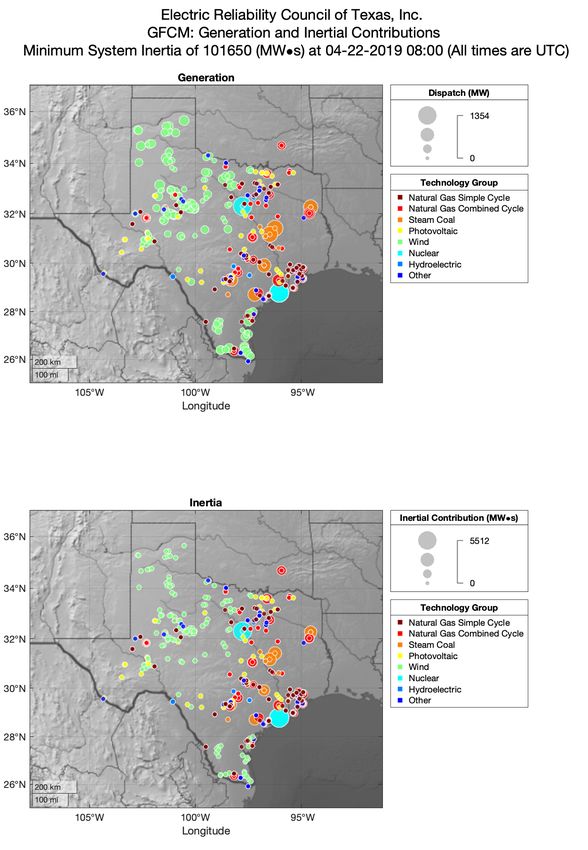
Figure 5 shows a spatial representation of inertia and net generation at the generator level for the
hours in which system inertia is estimated to obtain its minimum value. Similar graphics can be
produced with the GFCM for the hour in which wind generation is estimated to reach its highest
share of net generation. In this case, natural gas plants account for a large amount of the inertial
contributions made to the ERCOT grid. Careful observers of Fig. 5 may notice the peculiar
presence of an ERCOT plant located in Oklahoma. This is the Tenaska Kiamichi Generating
Station, which is capable of selling power to either ERCOT or the Southwest Power Pool (SPP)
[41, 42].
17NIST TN 2246
February 2023
Fig. 5. Balancing Authority Map at Annual Minimum Inertia
Figure 6 presents a box plot of the total system inertia values estimated for ERCOT in 2019 using
the GFCM. The distribution of hourly inertial contribution values attributable to combined cycle
natural gas plants, simple cycle natural gas plants, coal generation, load, and private use networks
is also displayed. Combined cycle plants are among the largest contributors to system inertia,
18NIST TN 2246
February 2023
both individually and as a group. Contributions to system inertia from conventional coal plants
appear smaller than those from load and private use networks, both of which are assumed to scale
with load. This fnding suggests that system operators may need to treat inertia from load and
private use networks commensurate with the fact that these sources account for a non-negligible
share of system inertia. The table included in Fig. 6 allows comparison of the GFCM estimate of
minimum system inertia, 101650 MW•s, with the target value of 134500 MW•s [40]. Note that
for the purpose of GFCM reporting, generator counts record wind farms with multiple turbines
as a single generator. The distribution of GFCM values for inertia from natural gas simple cycle
generation is a result of the model determining that such generators have higher marginal costs
than their combined cycle counterparts and are therefore allocated only when demand exceeds
levels which can be met by combined cycle generation alone. Heterogeneity in generator design
or grid conditions, if modeled with greater levels of granularity, could create a smoother transition
between technology groups along the merit order.
Fig. 6. Inertia Estimates Box Plot
19NIST TN 2246
February 2023
While system inertia and the minimum inertia event date differ between observed and modeled
values, the GFCM value for demand in that hour, 29860 MWh, is within 0.1 percent of the target
value of 29883 MWh. The remaining discrepancy between model and observed system inertia
may be driven by assumed patterns in PUN and load-based inertial contributions, neither of which
are directly observable by the analyst.
Table 2 presents summary statistics for hourly system inertia values estimated by the GFCM for
ERCOT from 2019 through 2021. The maximum, minimum, mean, and median system inertia
values decline over the three years. The standard deviation of hourly system inertia values de-
creased in 2020 before rising in 2021. The onset of the COVID-19 pandemic and the effects of
policy responses to the public health crisis cannot be eliminated as potential drivers of the observed
change in system inertia. The inertial contributions of demand-side and PUN resources remain a
source of model uncertainty, especially during a period of study for which signifcant changes to
economic organization occur. Additionally, rising input price volatility or increasing penetration
of intermittent resources may be suffcient to explain the rising standard deviation of system inertia
values in 2021.
Table 2. System Inertia Estimates: Summary Statistics for ERCOT 2019-2021
Year 2019 2020 2021
Maximum 520 942 508 819 499 569
Minimum 101 650 100 944 89 350
Mean 245 959 232 801 228 481
Median 227 755 216 049 207 692
Standard Deviation 87 662 82 069 90 014
System inertia summary statistics are valued in MW•s.
2.6. Model Validation
Validation of the GFCM is a process of obtaining and evaluating visualizations and metrics of
model performance. Ultimately, it is up to the analyst to determine whether the GFCM is perform-
ing suffciently well to justify its application to a given scenario. This section discusses several of
the model outputs produced to aid the analyst with model validation.
As a frst step, net generation is aggregated to the monthly generator level to harmonize the model
output with the variables presented in EIA Form 923. EIA Form 923 is not used at any other point
in the GFCM and is thus suited for model validation exercises. For a subset of generating units, we
obtain actual net generation values against which to validate model performance. We use monthly
aggregates because hourly generator level output data is proprietary. We are mainly interested in
determining whether the distributions of modeled net generation refect patterns observed in the
actual data. Because we do not differentiate assumed inertial constants within a given technology
group, matching a specifc generator value is less important than capturing the distribution of values
with satisfactory fdelity.
20NIST TN 2246
February 2023
Figure 7 presents a scatter plot of the observed (EIA Form 923) and modeled monthly data broken
out by a third variable indicating technology. Both axes are in log scale. The GFCM validation
function produces similar scatter plots coded by other tertiary variables, including the decade when
the generator began operating, the energy source code, the month of the year, industry classifcation
code, prime mover codes, and industrial sector. Proximity to the 45 degree line indicates a higher
degree of model agreement with reality at the generator level, though complete agreement at this
level of analysis is not necessary for the GFCM to capture system dynamics in synchronous inertial
contributions. These scatter plots are intended as a diagnostic tool for the analyst to identify and
understand any systematic departures of the model outcomes from the values reported in EIA Form
923.
Fig. 7. Observed and Modeled Monthly Net Generation by Technology
The scatter plots are useful for diagnosing potential model bias, but they mask the degree to which
the GFCM is able to recreate observed distributions of generating unit output. Figure 8 compares
the distribution of monthly net generation produced by the GFCM with that from EIA Form 923.
21You can also read