Benchmarking of numerical integration methods for ODE models of biological systems
←
→
Page content transcription
If your browser does not render page correctly, please read the page content below
www.nature.com/scientificreports
OPEN Benchmarking of numerical
integration methods for ODE
models of biological systems
Philipp Städter1,2,4, Yannik Schälte1,2,4, Leonard Schmiester1,2,4, Jan Hasenauer1,2,3* &
Paul L. Stapor1,2
Ordinary differential equation (ODE) models are a key tool to understand complex mechanisms
in systems biology. These models are studied using various approaches, including stability and
bifurcation analysis, but most frequently by numerical simulations. The number of required
simulations is often large, e.g., when unknown parameters need to be inferred. This renders efficient
and reliable numerical integration methods essential. However, these methods depend on various
hyperparameters, which strongly impact the ODE solution. Despite this, and although hundreds
of published ODE models are freely available in public databases, a thorough study that quantifies
the impact of hyperparameters on the ODE solver in terms of accuracy and computation time is still
missing. In this manuscript, we investigate which choices of algorithms and hyperparameters are
generally favorable when dealing with ODE models arising from biological processes. To ensure a
representative evaluation, we considered 142 published models. Our study provides evidence that
most ODEs in computational biology are stiff, and we give guidelines for the choice of algorithms and
hyperparameters. We anticipate that our results will help researchers in systems biology to choose
appropriate numerical methods when dealing with ODE models.
Systems biology aims at understanding and predicting the behavior of complex biological processes through
mathematical models1. In particular, ordinary differential equations (ODEs) are widely used to gain a holistic
understanding of the behaviour of such systems2. These ODE models are often derived from biochemical reaction
networks and stored/exchanged using the Systems Biology Markup Language (SBML)3 or Cell Markup Language
(CellML)4. Based on these community standards, large collections of published ODE models have been made
available to enhance reproducibility of scientific results, like BioModels5 and JWS6. These model collections allow
an analysis of typical properties of published ODE models of biological processes and are an excellent source for
method studies and method d evelopment7.
Most published models of biochemical reaction networks are non-linear and closed form solutions are not
available. Accordingly, numerical integration methods have to be employed to study them8. For this task, the
modeler has the choice between many possible numerical simulation algorithms, which have specific hyperpa-
rameters that can strongly impact the result. Key parameters are for instance the relative and absolute tolerance,
which determine the precision of the numerical solution. Too relaxed tolerances may lead to incorrect results,
while too strict tolerances may result in an unnecessarily high computation time, or may even lead to a failure
of ODE integration, if the desired solution accuracy cannot be a chieved9.
Various theoretical results about the reliability and the scaling behaviour of ODE solvers are available10.
However, to the best of our knowledge, there is no comprehensive study on the impact of ODE solver settings on
the simulation results and their reliability which focuses on models of biological processes. So far, case studies
using only single models or a very small number of models have been carried out, which demonstrate the need
for efficient implementations of ODE solvers (see, e.g.,8). In addition to this, various hypotheses on the general
properties of ODE models in systems biology exist, e.g., whether or not the underlying ODEs are expected to
be stiff—an ODE is (informally) called stiff, if it exhibits different time-scales, i.e., fast and slow dynamics are
described at the same time11,12. The absence of representative studies and statistical evaluations is surprising as
various tasks require large numbers of numerical simulations, rendering computation efficiency and numerical
1
Institute of Computational Biology, Helmholtz Zentrum München - German Research Center for Environmental
Health, 85764 Neuherberg, Germany. 2Center for Mathematics, Technische Universität München, 85748 Garching,
Germany. 3Faculty of Mathematics and Natural Sciences, University of Bonn, 53113 Bonn, Germany. 4These
authors contributed equally: Philipp Städter, Yannik Schälte and Leonard Schmiester. *email: jan.hasenauer@
uni‑bonn.de
Scientific Reports | (2021) 11:2696 | https://doi.org/10.1038/s41598-021-82196-2 1
Vol.:(0123456789)www.nature.com/scientificreports/
robustness an important topic. In particular when performing parameter estimation, a model has to be simulated,
i.e., the underlying ODE has to be solved, thousands to millions of times8,13. Indeed, it has recently been pointed
out that the ODE solver is actually a crucial hyperparameter, which often remains u nconsidered14. Hence, study-
ing these questions on a wide set of real world applications is of high importance for many modeling applications.
In this work, we benchmark numerical integration methods and their hyperparameters. We established a
benchmark collection of 142 models from the two freely accessible databases BioModels5,15 and JWS Online6,
which covers a broad range of different properties. These models were simulated using various ODE solver algo-
rithms implemented in the ODE solver toolboxes C VODES16 from the SUNDIALS suite9 and the ODEPACK
17
package , which are possibly the most widely used software package to integrate ODEs in systems biology. We
investigated various combinations of ODE integration algorithm, non-linear solver employed in implicit multi-
step methods, linear solvers employed within the non-linear solver, and relative and absolute error tolerances.
By analyzing the computation time and the failure rate, we derived guidelines for the tuning of ODE solvers in
systems biology, which facilitate fast and reliable simulation of the corresponding ODE systems.
Results
To analyze combinations of algorithms and hyperparameters, we considered the ODE solvers from the SUNDI-
ALS package CVODES9,16, which implement implicit multi-step methods for numerically solving an initial value
problem, i.e., an ODE with initial conditions and offer a variety of hyperparameters. We furthermore included
the ODEPACK17 package in our analysis, which uses the multi-step algorithm LSODA, which adaptively switches
between methods stiff and nonstiff ODEs for numerical integration18. CVODES and ODEPACK are used in
multiple systems biology t oolboxes19–22 and are therefore particularly relevant.
An initial value problem is solved by iterative time-stepping, following a specific integration a lgorithm10,23,
(see Methods, Numerical integration methods for ODEs for more details). In each time step, a non-linear problem
is solved via a fixed-point iteration or a sequence of linear problems. These are solved until a previously defined
precision, given by absolute and relative error tolerances, is fulfilled.
CVODES offers the following hyperparameters:
1. Integration algorithm:
(a) Adams-Moulton (AM): implicit multi-step method of variable order 1 to 12, chosen automatically
(b) Backward Differentiation Formula (BDF): implicit multi-step method of variable order 1 to 5, chosen
automatically
2. Non-linear solvers:
(a) Functional: solution to the non-linear problem directly via a fixed-point method
(b) Newton-type: linearization of the non-linear problem
3. Linear solver (only when using Newton-type non-linear solver):
(a) DENSE: dense LU decomposition
(b) GMRES: iterative generalized minimal residual method on Krylov subspaces
(c) BICGSTAB: iterative biconjugate gradient method on Krylov subspaces
(d) TFQMR: iterative quasi-minimal residual method on Krylov subspaces
(e) KLU: sparse LU decomposition
4. Error tolerances: upper bounds for the absolute and relative error made in each time-step
ODEPACK offers absolute and relative error tolerances as only hyperparameters, with LSODA switching auto-
matically between a BDF algorithm using a Newton-type method with dense LU decomposition in the stiff and
an AM algorithm using a functional iterator in the nonstiff case.
We will call a combination of these hyperparameters a solver setting.
As it is still unclear which solver settings are best suited for models of biochemical reaction networks, we
performed a comprehensive empirical study to answer this question. Therefore, we considered for CVODES all
20 possible combinations of integration algorithm, non-linear solver, and linear solver with 7 different error
tolerances combinations. For ODEPACK, we used the same 7 combinations of error tolerances. Furthermore,
we considered 36 error tolerance combinations in an in-depth tolerance study for CVODES, yielding in total
176 (= 20 × 7 + 7 + (36 − 7)) different solver settings.
As performance characteristics of a solver setting, we consider the following two criteria:
1. Integration failures: These failures may occur if either the dynamics of the system become too stiff or if the
state of the system diverges. In these cases, the requested numerical accuracy per integration step cannot be
achieved by a solver setting and the (adaptively chosen) step-size falls below machine precision and integra-
tion gets stuck.
2. Computation times: The total computation time is determined by the number of steps the solver takes and
their individual computation times. Both quantities can vary heavily depending on the solver settings.
Scientific Reports | (2021) 11:2696 | https://doi.org/10.1038/s41598-021-82196-2 2
Vol:.(1234567890)www.nature.com/scientificreports/
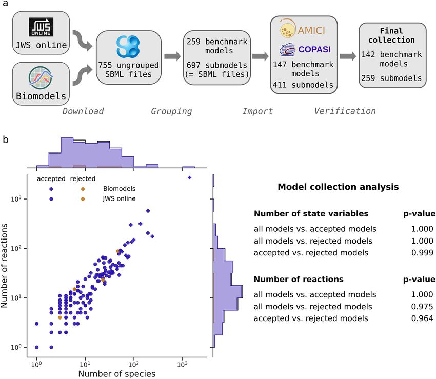
Figure 1. Model collection. (a) Workflow of collecting models for the benchmark collection. Models were
downloaded, grouped according to their number of species and reactions, the author name and year of their
publication, imported with AMICI and COPASI, and simulation results were compared to reference trajectories
using multiple solver settings. (b) Basic properties (number of state variables and reactions) of the benchmark
collection models, as joint scatter plot, indicating the number of accepted, rejected, and the total number of
grouped models. The distributions of the numbers of state variables and numbers of reactions were compared
for all imported models, vs. accepted models vs. rejected models by a Kolmogorov-Smirnov test, to assess a
possible bias due to the filtering step.
A comprehensive model collection allows the systematic benchmarking of hyperparame-
ters. For a comprehensive study on a variety of ODE models, we downloaded all SBML models from the
JWS database6. As all of those models had less than 100 state variables, we complemented them with a set of the
largest models from the BioModels database5. To simulate these models using CVODES, we imported them with
AMICI (Advanced Multi-language Interface to CVODES and IDAS22), which performs symbolic preprocess-
ing and creates and compiles executable code for each model. For simulation with the LSODA algorithm from
ODEPACK, we furthermore imported these model with COPASI19. As neither AMICI nor COPASI support all
features of SBML, only a subset of the models could be imported with both toolboxes. These SBML models were
then grouped together, to avoid counting variations of the same model multiple times, yielding 148 benchmark
models comprising 411 SBML files: One benchmark model may hence consist of multiple submodels, i.e., SBML
files. Computation times were averaged over the submodels of a benchmark model. We considered the simula-
tion of a benchmark model failed if the simulation of at least one of its submodels failed. To ensure a proper
comparison, we verified the correctness of the simulated trajectories (Fig. 1a, Supplementary Fig. S1), based on
reference solutions. After this filtering step, we were left with 142 benchmark models comprising 259 submod-
els, of which a majority comprises between 10 and 100 state variables and reactions (Fig. 1b). A Kolmogorov-
Smirnov test on the distributions of the numbers of model species and reactions comparing the accepted with
Scientific Reports | (2021) 11:2696 | https://doi.org/10.1038/s41598-021-82196-2 3
Vol.:(0123456789)www.nature.com/scientificreports/
Figure 2. Non-linear solver. Comparison of functional and Newton-type non-linear solver in terms of failure
rate. Each point represents the failure rate when simulating all models for a given combination of integration
algorithm, non-linear solver, linear solver and error tolerances.
the rejected models yielded little evidence for these distributions to be different (p-values of 0.999 and 0.964 for
species and reactions, respectively). For details on the construction of the benchmarking collection (e.g., source
of reference solutions) we refer to the Methods, Creation of the ODE solver benchmark collection.
Newton‑type method outperforms functional iterator when solving the non‑linear prob-
lem. Using the 142 benchmark models, we analyzed the impact of different hyperparameters on the perfor-
mance of numerical ODE solvers. As we expected the combination of the non-linear and linear solver to strongly
impact the reliability of the numerical ODE integration, we decided to first study this aspect.
We compared the rate of integration failure for the two available non-linear solvers—the functional iterator
and the Newton-type solver—for both ODE integration algorithms in CVODES (AM and BDF), all available
linear solvers and a set of heterogeneous error tolerances, motivated by commonly used ODE solver settings.
LSODA uses a fixed implementation for solving the nonlinear problem which can not be altered.
This comparison revealed that the Newton-type method performs better than the functional iterator: While
the functional iterator, which does not rely on a linear solver, failed on average for 10–15% of the models, the
Newton-type method failed substantially less (Fig. 2). Indeed, in combination with the BDF integration algo-
rithm, we observed for all but the dense direct linear solver DENSE a failure rate of roughly 5% of the models.
Overall, the BDF integration algorithm appeared to be less prone to integration failure than the AM method.
Fisher’s exact tests showed that the difference was not significant for the functional iterator (with a p-value of
0.215 for the linear solver KLU), but significant when using the Newton-type method (p-value of 1.35 · 10−5 for
KLU). The LSODA algorithm outperformed the best results of the BDF algorithm and the Newton-type method
(p-values using Fisher’s exact test of 7.43 · 10−6 for LSODA vs. KLU and 0.025 for LSODA vs. BICGSTAB). This is
surprising, as it uses a Newton-type method with dense linear solver and relies on the BDF algorithm—a setting
which performed clearly worse in CVODES. This suggests that the implementation of the non-linear and linear
solver in ODEPACK is superior to the one in CVODES for the considered models class.
These results can be considered as hint that many models are stiff, as the AM algorithm is less tailored to
models exhibiting stiff d ynamics23 than the BDF or the LSODA algorithm.
Interestingly, some models could only be integrated using an iterative linear solver, while another small set
of models could only be integrated using a direct linear solver. This suggests that it may be crucial to have the
choice between different linear solvers in certain applications. Furthermore, we observed that the failure rate
tended to increase for stricter error tolerances. The highest failure rate was observed for the Newton-type method
in combination with the dense linear solver. For all other linear solvers, the Newton-type method is less prone
to integration failure than the functional iterator and also more efficient in terms of computation time (Supple-
mentary Fig. S2). Thus, we focus in the following only on results for the Newton-type method.
The sparse direct linear solver from CVODES scales best. To determine the performance of the dif-
ferent linear solvers, we assessed their computation times. For the BDF algorithm, we found that the dense direct
solver exhibited the worst scaling behavior with respect to the number of state variables, followed by the iterative
solver TFQMR (Fig. 3a). The iterative linear solvers GMRES and BICGSTAB showed a roughly linear scaling
behavior for the BDF algorithm of the computation time with the model size. The sparse direct solver KLU had
the best scaling behavior. For the BDF algorithm with the linear solver KLU, the complexity of the numerical
integration increased roughly by a factor of four when the model size increased by a factor of five.
Assessing the computation times across models for different error tolerances confirmed that the sparse direct
linear solver KLU performed best for every tolerance combination (Fig. 3b, Supplementary Figs. S3, S4, and S5),
Scientific Reports | (2021) 11:2696 | https://doi.org/10.1038/s41598-021-82196-2 4
Vol:.(1234567890)www.nature.com/scientificreports/
Figure 3. Linear solvers. Scaling behavior and computation time comparison of the linear solvers and
integration algorithms. (a) Each point depicts the simulation time of one model (median of 25 repetitions) with
one solver setting: BDF integration algorithm, Newton-type non-linear solver, one tolerance combination, and
one linear solver (which are color-coded). Results are shown for seven tolerance combinations and five linear
solvers, meaning there are 35 points for each model. The accompanying linear regressions display the scaling
behavior with respect to the number of state variables. (b) Box plot of the simulation times, separated by the
tolerance combination in addition to the linear solver, using the BDF integration algorithm and the Newton-
type non-linear solver. (c) Scaling behavior of the different integration algorithms using the Newton-type
method and the direct linear solvers with the same setup as in subfigure (a). (d) Box plot of the simulation times
for the different integration algorithms using the Newton-type method and the direct linear solvers with the
same setup as in subfigure b.
followed by the two iterative linear solvers GMRES and BICGSTAB, which showed comparable computation
times. The dense linear solver DENSE yielded the highest computation times. As expected, stricter error toler-
ances consistently led to an increase of computation time for all employed solver settings.
When comparing the scaling behavior of the direct linear solvers across integration algorithms, we saw that
KLU performed best and DENSE performed worst (both from CVODES, Fig. 3c), while the LSODA imple-
mentation had an intermediate scaling. Overall, the combination of BDF and KLU was the best performer, also
in terms of computation time (Fig. 3d). In general, the scaling behavior for the AM integration algorithm was
slightly worse than for the BDF algorithm (Supplementary Figs. S3, S4, and S5).
Choosing error tolerances is a trade‑off between accuracy, reliability, and computation
time. In a next step, we studied the effect of the error tolerances on the computation time. As the Newton-
type non-linear solver with the sparse direct linear solver KLU outperformed the other combinations, we used
this combination to analyze the impact of the absolute and relative error tolerances on computation time and
failure rate. For an extensive tolerance study, not only the hitherto seven, but 36 tolerance combinations were
analyzed, covering a broad spectrum. As upper bounds for the relative and absolute tolerances we used 10−6, as
Scientific Reports | (2021) 11:2696 | https://doi.org/10.1038/s41598-021-82196-2 5
Vol.:(0123456789)www.nature.com/scientificreports/
Figure 4. Integration error tolerances. Comparison of 36 combinations of absolute and relative error tolerances.
All models were simulated using the BDF integration algorithm, the Newton-type non-linear solver, and the
linear solver KLU, for each tolerance combination. (a) Relative simulation times, normalised by those for
absolute and relative error tolerances (10−6 , 10−6 ). (b) The corresponding failure rates.
more relaxed tolerances provided an insufficient agreement with the reference trajectories (see Methods, Crea-
tion of the ODE solver benchmark collection and Supplementary Fig. S1).
To compare computation times across all models, we analyzed CPU time ratios. The computation time for
each model and each error tolerance combination was normalized by the computation time for the most relaxed
tolerance combination, i.e., absolute and relative tolerance of 10−6 (Fig. 4a, Supplementary Fig. S6). We found
that for most models, the computation time increases with the enforced accuracy. Yet, we found some models,
which were simulated faster when mildly restricting the error tolerances, indicating a non-trivial relation. Apart
from those exceptions, the median CPU time increased monotonically by roughly an 11-fold when restricting
the absolute and relative error tolerances from 10−6 to 10−16. Hence, restricting the requested error tolerances
by ten orders of magnitude increased the median computation time by about one order of magnitude, which
was less than we had expected. Furthermore, strict relative error tolerances tended to have a bigger impact on
the computation time and the failure rate than strict absolute tolerances. While the overall failure rate mildly
decreased when restricting the error tolerances to a range between 10−8 and 10−12, it increased markedly when
both error tolerances were set to very strict values at the same time (Fig. 4b).
Fully implicit algorithms are the best choice for most models. Since we have seen noticeable differ-
ences in their behavior, we compared the integration algorithms AM, BDF, and LSODA for each model individu-
ally regarding their computation time and failure rate. Therefore, we used again the seven tolerance combina-
tions which we employed for the analysis of the non-linear and the linear integration algorithms, together with
the Newton-type non-linear solver and the KLU linear solver for AM and BDF.
We observed that for most models and settings, the BDF algorithm was faster than the AM algorithm (roughly
50% vs. 37%, Fig. 5a). For a number of models, especially for the larger ones, BDF was faster by almost two orders
of magnitude when compared to AM. In contrast, AM outperformed BDF by at most a factor of 5 (Fig. 5b).
Importantly, the BDF algorithm was not only computationally more efficient, but showed also the lower failure
rate: For about 6% of the settings, both algorithms failed to integrate the ODE. For an additional 5.7% of the
cases, BDF could still integrate the ODE although AM failed, while the opposite was true in only 0.1% of the
cases. Hence, the AM algorithm failed about twice as often to integrate the ODE system as the BDF algorithm.
When comparing AM and BDF with LSODA, we found that for the majority of models, AM and BDF
markedly outperformed LSODA in terms of computation time: AM was faster for 74% of the models (vs. 13%
for LSODA, (Fig. 5c,d) and BDF was faster for 89% of the models (vs. 3.8% for LSODA, (Fig. 5e,f). For certain
models, AM outperformed LSODA by up to a 70-fold, while LSODA outperformed AM by up to a 30-fold. BDF
was faster by up to a 500-fold, while LSODA achieved to outperform BDF by at most a 4-fold. In particular for
models with more than 15 state variables, BDF was always faster than LSODA. A possible explanation for the
lower computation times of the algorithms implemented in CVODES is the sparse linear solver in the Newton-
type method, and the fact that AMICI provides an analytically calculated Jacobian matrix to CVODES, whereas
Scientific Reports | (2021) 11:2696 | https://doi.org/10.1038/s41598-021-82196-2 6
Vol:.(1234567890)www.nature.com/scientificreports/
Figure 5. Comparison of integration algorithm (a) Each scatter point shows the computation time for a model
using the AM (x-axis) or BDF (y-axis) algorithm with the Newton-type non-linear solver, the linear solver
KLU and one out of the seven tolerance combinations. Darker colors represent a higher scatter point density.
(b) Computation time for AM divided by the computation time for BDF with respect to the number of state
variables, using the color coding from subfigure A. (c) Comparison of the LSODA algorithm (x-axis) with the
AM algorithm (y-axis) with the same setup as in a. (d) Computation time ratios for the LSODA devided by the
AM algorithm, using the color coding from c. (e) Comparison of the LSODA algorithm (x-axis) with the BDF
algorithm (y-axis) with the same setup as in a. (f) Computation time ratios for the LSODA devided by the BDF
algorithm, using the color coding from e.
Scientific Reports | (2021) 11:2696 | https://doi.org/10.1038/s41598-021-82196-2 7
Vol.:(0123456789)www.nature.com/scientificreports/
ODEPACK computes the Jacobian by finite differences in COPASI, which is computationally more demanding
for larger systems.
It is important to note that AM and BDF suffered from higher rates of integration failure than LSODA: BDF
failed almost three times as often as LSODA (6.1% vs. 2.1%), AM about more than five times as often (11.8%
vs. 2.1%). However, these failure rates improved for AM and BDF when using one of the iterative linear solver
BICGSTAB (AM: 9.3%, BDF: 3.5%), such that BDF was almost on par with LSODA (Supplementary Fig. S7).
Using the linear solver GMRES, BDF still showed a good performance, while AM worked less well (Supplemen-
tary Fig. S8). Hence, LSODA is overall clearly slower than the CVODES implementation of BDF with its sparse
linear solver, but more robust to integration failure.
Discussion
Modeling with ODEs is among the most popular approaches to develop a holistic understanding of cellular
processes in systems biology. Here, we collected a set of 142 benchmark ODE models collected from publica-
tions and used them to carry out a comprehensive study on the most essential hyperparameters of numerical
ODE solvers. To the best of our knowledge, this is the first extensive study focusing on ODE integration itself,
investigating a total of 176 ODE solver settings. The use of a large number of established models makes it highly
relevant to the community. Although the optimal choice of hyperparameters is model dependent, our findings
allow to draw some general conclusions:
Firstly, we found that, in general, error tolerances should not be relaxed beyond the value of 10−6 , as oth-
erwise simulation results tend to deviate markedly from results of more accurate computations. However, too
strict error tolerances substantially increase the computation time and, more importantly, can lead to failure of
ODE integration. We conclude that for most models, error tolerances between 10−8 and 10−14 are a reasonable
choice, with absolute error tolerances being stricter than relative error tolerances, at least for the ODE solver
implementation considered in this study.
Secondly, we observed that for more than 60% of the models, the BDF integration algorithm was superior
to the AM integration algorithm in the implementation of CVODES. As the AM algorithm is generally recom-
mended for mildly stiff problems and BDF is more tailored to stiff s ystems23, this implies that most ODE models
in systems biology show substantial stiffness. Stiffness was already hypothesized for ODEs arising from biologi-
cal systems11,12, but to the best of our knowledge, this was never quantified. Hence, our results suggest that fully
implicit methods for ODE integration with adaptive time-stepping and error control are necessary to obtain
reliable results, except for special cases, where clear motivations for other approaches can be given. We also want
to stress that all ODE models were analyzed at the reported parameter values, for which ODE integration is sup-
posed to work well. However, these parameters often have to be estimated first, by evaluating the ODE at various
parameters and comparing model simulations with measurement d ata13,24. During this estimation process, the
model does often not yet reflect a realistic behavior and in our experience stiffness is encountered substantially
more often. Hence, in parameter estimation, stiffness is likely to be even more present.
Thirdly, when comparing algorithms for solving the non-linear and the linear problem within implicit inte-
gration methods, we found that the fastest setting is using a Newton-type method for the non-linear problem
and a sparse direct solver for the linear problem (in our case KLU), in particular with a better scaling behavior
towards higher-dimensional models. This setting was also among the most reliable settings when comparing
ODE integration failure, but was outperformed by iterative linear solvers and by the LSODA implementation
from ODEPACK. In contrast, the dense direct linear solver from the CVODES implementation showed the worst
performance. Furthermore, it was pointed out that for stiff ODE systems, Newton-type non-linear solvers tend
to be superior to fixed-point m ethods25, which we can underline by our findings.
In our opinion, a good default setting for most models should be an ODE solver using the BDF (or LSODA)
algorithm, together with a Newton-type approach for the non-linear, and a sparse direct solver for the linear
problem. If this leads to integration failure, an iterative linear solver—in our case, BICGSTAB worked best—may
be a promising alternative. It may be helpful to check for a given model whether the AM integration algorithm
reduces the computation time, as this is generally model dependent. However, model simulations should then
ideally be verified using a BDF algorithm to ensure accuracy.
While this study focused on numerically solving ODE systems, a valuable extension would be assessing the
performance of ODE integration when performing it with forward and adjoint sensitivity a nalysis26. This is a
typical setting when estimating unknown model parameters, as sensitivities are needed to compute the gradient of
an objective function which depends on the ODE s olution13. It would be particularly interesting to see whether it
could be inferred when forward and when adjoint sensitivity analysis should be used: Although forward sensitiv-
ity analysis is more commonly used and may be superior for small models, adjoint sensitivity analysis is known
to be more efficient for large models26,27. Yet, no clear rule for deciding between those two approaches could be
derived so far. The respective sensitivity equations may also change in particular the stiffness of the ODE, which
may impact optimal hyperparameters.
Moreover, the multi-step algorithms in CVODES and ODEPACK could be compared to other approaches,
such as the (implicit) single-step algorithms which are provided in, e.g., the toolbox F ATODE28. Another direc-
tion of future research may be accelerating computations via GPUs, which can be advantageous for certain use
cases29. Additionally, it should be noted that many ODE solver toolboxes allow to specify error tolerances for
each state variable of the ODE system separately. If prior knowledge on the trajectories of the model simulation
is available, this option may be exploited to either improve accuracy or speed up model simulation.
In conclusion, we are certain that the presented study will be helpful for both modelers and toolbox develop-
ers, when choosing hyperparameters for ODE solvers to yield both reliable and efficient simulations.
Scientific Reports | (2021) 11:2696 | https://doi.org/10.1038/s41598-021-82196-2 8
Vol:.(1234567890)www.nature.com/scientificreports/
Methods
Numerical integration methods for ODEs. An ODE model describes the dynamics of a vector of state
variables x(t) ∈ Rnx with respect to time t, model parameters θ , and input parameters u. The time evolution is
given by a vector field f:
d
x(t) = f (x(t), θ, u), x(0) = x0 (θ, u). (1)
dt
As typically the solution x(t) cannot be computed analytically, we consider in this study different numerical
integration methods which proceed along the time course step by step: Starting from time t0 and state x0 , an
approximation xk of the state x(tk ) at the k-th time-step tk is computed from the states and the vector fields at
previous time points. In so-called multi-step methods, the s previous time-steps of the ODE solver tk−1 , . . . , tk−s
are used, where s ∈ N fixes the order of the method. The most general form of a multi-step method is:
s
s
xk = αj xk−j + hk βj f (tk−j , xk−j , θ, u) (2)
j=1 j=0
The difference hk = tk − tk−1 defines the time-step length, and the coefficients αj and βj determine the exact
algorithm. When β0 = 0, the method is explicit, otherwise implicit. Generally, implicit algorithms are considered
to be better suited for ODE systems with so-called stiff d ynamics23.
For implicit methods and non-linear vector fields f, a non-linear problem has to be solved to determine xk .
In order to solve the non-linear problem, either a fixed-point iteration can be used, which tries to approximate
f (tk , x(tk ), θ, u) step by step, or a Newton-type method can be employed, which reduces Equation (2) to a series
of linear problems, which can be denoted as:
(3)
I − γ ∇x f (tk , xk , θ, u) �xk = −f (tk , xk , θ, u),
where is the unit matrix I , γ > 0 a relaxation constant and ∇x f (tk , xk , θ, u) the Jacobian of the right hand side.
In the latter case, algorithms for solving linear problems have to be used repeatedly. Here, we consider two
approaches: Direct approaches, which try to solve Equation (3) by factorization of the matrix I − γ ∇x f (tk , xk , θ, u)
(such as LU factorization); and iterative approaches, such as Krylov subspace methods, which try to compute
x by a sequence of improving approximations x 0 , x 1 , . . . , x m , until x m solves Equation (3) up to a previously
defined accuracy.
Statistical tests. To perform the statistical tests, we used the implementation of the stats package in the
SciPy toolbox (release 1.4.1). The Kolmogorov-Smirnov tests were performed as a two-sample test using the
function ks_2samp, Fisher’s exact tests were performed using the function fisher_exact.
High performing software packages for ODE integration. It has been shown in several studies that
it is critical to use high-performance ODE solver toolboxes written in compiled languages such as C++ or FOR-
TRAN, since those have shown to reduce computation time by two to three orders of m agnitude8,30. For this rea-
son, we focused on the C-based ODE solvers in CVODES, which is part of the SUNDIALS solver package9 and
the LSODA algorithm from the FORTRAN-based ODEPACK suite. These solvers are used in several established
toolboxes, e.g., D ata2Dynamics20, libroadrunner21, COPASI19, or A
MICI22 and represent probably the two most
widely used implementations in the field of systems biology. Appropriate alternatives might be in our opinion
other solver toolboxes written in compiled languages, such as the FORTRAN-based FATODE implementation28
or the FORTRAN-based ODEPACK implementation17, or reimplementations of these. Additionally, Julia writ-
ten toolboxes, such as DifferentialEquations.jl could also be valuable a lternatives31. For applications which ben-
efit from a high degree of parallelization, GPU acceleration may also be beneficial. Approaches in this direction
are implemented in, e.g., the toolboxes LASSIE32 and cupSODA29,33.
Setup of the numerical experiments. All numerical simulations were repeated 25 times to avoid outli-
ers in the computation time. Afterwards, the median values of all these computation times were stored. Since a
repeated simulation using the same solver setting does not change the success of the simulation, this informa-
tion was stored after the first simulation. In total, 49,984 data points for computation time and success of the
simulation were created. These were then analyzed and displayed in different ways to illustrate the impact of the
hyperparameters on simulation time and reliability. The whole dataset and the code of the implementation is
made available at https://doi.org/10.5281/zenodo.4013853 and as a repository on GitHub at https://github.com/
ICB-DCM/solverstudy. The study was performed on a laptop with Ubuntu 20.04.1 LTS operating system, an
Intel Core i7-8565U CPU with a maximal capacity of 4.60GHz, and 40GB RAM.
Creation of the ODE solver benchmark collection. As a first step, we downloaded all models from
the JWS database (date of download: June 17, 2019). As these models were comparably small, we complemented
this collection by a set of larger models from the BioModels database (date of download: June 24, 2019) and a
particularly large SBML model of cancer s ignalling34, available at https://github.com/ICB-DCM/CS_Signalling
_ERBB_RAS_AKT (commit 365e0be, date of download: June 24, 2019). These larger models allowed us to also
assess the scaling behavior of computation times with respect to the size of the ODE models. In total, we thus
downloaded 755 SBML models.
Scientific Reports | (2021) 11:2696 | https://doi.org/10.1038/s41598-021-82196-2 9
Vol.:(0123456789)www.nature.com/scientificreports/
On JWS, the models are grouped as SED-ML models35. A SED-ML model consists of possibly multiple SBML
(sub-)models, may contain changes to be performed on the SBML (sub-)models, and contains time frames for
specific simulations. The SBML models coming from JWS were hence adapted according to the specifications
in the SED-ML files and simulation time frames were extracted and saved. For the models from BioModels, we
deduced possible time frames from figures in the publications or by visual inspection of the state trajectories and
trying to determine reasonable settings. Afterwards, the adapted SBML models were grouped according to the
first author and the year of the corresponding publication, the number of chemical species, and the number of
reactions. If these four quantities coincided for multiple SBML models, we classified them as submodels of one
benchmark model, in order to avoid biasing results by including the same model with minor variations multiple
times. After this regrouping step, we were left with 259 benchmark models and 697 submodels.
The SBML models were then imported with AMICI (version 0.10.19, commit d78010f) leaving us with 148
benchmark models consisting of 455 submodels. The main reason for this loss is that AMICI did not support
all features of SBML, such as rate rules or assignment rules for parameters or species. Those remaining models
were also imported with COPASI, which reduced the overall number of accepted models to 147 benchmark
models with 411 submodels. We assessed the correctness of the simulated state trajectories based on reference
trajectories. For the models from JWS, reference trajectories were generated with the JWS built-in simulation
routine, comprising 101 simulation time points along the trajectory. For the models from BioModels, we gener-
ated reference trajectories with the COPASI toolbox19 comprising 51 simulation time points, using the strictest
error tolerances which still allowed a successful integration of the ODE system. As the COPASI simulator is
probably the most widely used ODE solver implementation in the field of systems biology, we considered this
the most reliable solution. Additionally, state trajectories were also compared by visual inspection.
All models were then simulated with AMICI using all 140 ODE solver settings from the main study and with
COPASI using all 7 solver settings from the main study. We also tested whether a higher maximum number of
ODE solver steps affected the result, but did not find a substantial impact. An SBML (sub-)model was assumed
to be correctly simulated, if for each time point of each simulated state trajectory, the absolute or relative error
(i.e., the mismatch between the reference trajectory and the simulation) were below a predefined acceptance
threshold for at least one solver setting for either AMICI or COPASI. We investigated the number of accepted
models in dependence of the acceptance threshold for various absolute and relative error tolerances (Supple-
mentary Fig. S1). For too strict acceptance thresholds, all models were rejected, but when simulating with high
accuracy, gradually increasing the threshold led to a plateau of accepted models for thresholds between 10−5 and
10−3. When increasing the acceptance threshold further, the number of accepted models grew until eventually
all models were accepted. We interpreted the plateau of models at threshold values around 10−4 as those models
which could be simulated correctly with sufficient accuracy and hence fixed the final acceptance threshold to a
value of 10−4 . Models were typically rejected, if the adaptation of the SBML file based on a corresponding SED-
ML file did not work properly. This is the reason why the filtering step strongly reduced the number of SBML
(sub-)models in the collection, while the number of benchmark models was less affected.
This procedure resulted in accepting a total of 259 SBML models, which were grouped to 142 benchmark
models.
Received: 4 September 2020; Accepted: 8 January 2021
References
1. Kitano, H. Computational systems biology. Nature 420, 206–210 (2002).
2. Klipp, E., Herwig, R., Kowald, A., Wierling, C. & Lehrach, H. Systems biology in practice (Wiley-VCH, Weinheim, 2005).
3. Hucka, M. et al. The systems biology markup language (SBML): a medium for representation and exchange of biochemical network
models. Bioinformatics 19, 524–531 (2003).
4. Cuellar, A. A. et al. An overview of CellML 1.1, a biological model description language. Simulation 79, 740–747 (2003).
5. Li, C. et al. BioModels database: an enhanced, curated and annotated resource for published quantitative kinetic models. BMC
Syst. Biol. 4, 92 (2010).
6. Olivier, B. G. & Snoep, J. L. Web-based kinetic modelling using JWS online. Bioinformatics 20, 2143–4 (2004).
7. Hass, H. et al. Benchmark problems for dynamic modeling of intracellular processes. Bioinformatics 35, 3073–3082 (2019).
8. Maiwald, T. & Timmer, J. Dynamical modeling and multi-experiment fitting with potterswheel. Bioinformatics 24, 2037–2043
(2008).
9. Hindmarsh, A. C. et al. SUNDIALS: suite of nonlinear and differential/algebraic equation solvers. ACM Trans. Math. Softw. 31,
363–396 (2005).
10. Ascher, U. M. & Petzold, L. R. Computer methods for ordinary differential equations and differential-algebraic equations (SIAM,
Philadelphia, 1998).
11. Garfinkel, D., Marbach, C. B. & Shaprio, N. Z. Stiff differential equations. Ann. Rev. Biophys. Bioeng. 6, 525–542 (1977).
12. Mendes, P. et al.Computational Modeling of Biochemical Networks Using COPASI, chap. 2. Part of the Methods in Molecular Biology
(Humana Press, 2009).
13. Raue, A. et al. Lessons learned from quantitative dynamical modeling in systems biology. PLoS ONE 8, e74335 (2013).
14. Kreutz, C. Guidelines for benchmarking of optimization-based approaches for fitting mathematical models. Genome Biol. 20, 281
(2019).
15. Malik-Sheriff, R. S. et al. BioModels-15 years of sharing computational models in life science. Nucleic Acids Res. 48, D407–D415
(2019).
16. Cohen, S. D., Hindmarsh, A. C. & Dubois, P. F. Cvode, a stiff/nonstiff ode solver in c. Comput. Phys. 10, 138–143 (1996).
17. Hindmarsh, A. C. Odepack, a systematized collection of ode solvers. Sci. Comput. 55–64, (1983).
18. Petzold, L. Automatic selection of methods for solving stiff and nonstiff systems of ordinary differential equations. SIAM. J. Sci.
Stat. Comput. Stat. Comput. 4, 136–148 (1983).
19. Hoops, S. et al. COPASI - a complex pathway simulator. Bioinformatics 22, 3067–3074 (2006).
Scientific Reports | (2021) 11:2696 | https://doi.org/10.1038/s41598-021-82196-2 10
Vol:.(1234567890)www.nature.com/scientificreports/
20. Raue, A. et al. Data2Dynamics: a modeling environment tailored to parameter estimation in dynamical systems. Bioinformatics
31, 3558–3560 (2015).
21. Somogyi, E. T. et al. libRoadRunner: a high performance SBML simulation and analysis library. Bioinformatics 31, 3315–3321
(2015).
22. Fröhlich, F., Weindl, D., Schälte, Y., Pathirana, D., Paszkowski, Ł., Lines, G. T., Stapor, P. & Hasenauer, J. AMICI: High-performance
sensitivity analysis for large ordinary differential equation models. arXiv:2012.09122 (2020).
23. Hairer, E. & Wanner, G. Solving ordinary differential equations II. Stiff. Differ. Algebr. Probl. 14, (1996).
24. Villaverde, A. F., Froehlich, F., Weindl, D., Hasenauer, J. & Banga, J. R. Benchmarking optimization methods for parameter estima-
tion in large kinetic models. Bioinformatics bty736 (2018).
25. Norsett, S. P. & Thomsen, P. G. Switching between modified newton and fixed-point iteration for implicit ODE-solvers. BIT Numer.
Math. 26, 339–348 (1986).
26. Fröhlich, F., Kaltenbacher, B., Theis, F. J. & Hasenauer, J. Scalable parameter estimation for genome-scale biochemical reaction
networks. PLoS Comput. Biol. 13, e1005331 (2017).
27. Sengupta, B., Friston, K. J. & Penny, W. D. Efficient gradient computation for dynamical models. NeuroImage 98, 521–527 (2014).
28. Zhang, H. & Sandu, A. FATODE: A library for forward, adjoint, and tangent linear integration of ODEs. SIAM J. Sci. Comput. 36,
C504–C523 (2014).
29. Nobile, M., Cazzaniga, P., Besozzi, D. & Mauri, G. GPU-accelerated simulations of mass-action kinetics models with cupSODA.
J. Supercomput. 69, 17–24 (2014).
30. Kapfer, E.-M., Stapor, P. & Hasenauer, J. Challenges in the calibration of large-scale ordinary differential equation models. IFAC-
PapersOnLine 52, 58–64 (2019).
31. Rackauckas, C. & Nie, Q. Differentialequations.jl–a performant and feature-rich ecosystem for solving differential equations in
julia. J. Open Res. Softw5 (2017).
32. Tangherloni, A., Nobile, M., Besozzi, D., Mauri, G. & Cazzaniga, P. LASSIE: simulating large-scale models of biochemical systems
on GPUs. BMC Bioinf. 18, (2017).
33. Harris, L. et al. GPU-powered model analysis with PySB/cupSODA. Bioinformatics 33, 3492–3494 (2017).
34. Fröhlich, F. et al. Efficient parameter estimation enables the prediction of drug response using a mechanistic pan-cancer pathway
model. Cell Syst. 7, 567-579.e6 (2018).
35. Waltemath, D. et al. Reproducible computational biology experiments with SED-ML - The Simulation Experiment Description
Markup Language. BMC Syst. Biol. 5, (2011).
Acknowledgements
We want to thank Jacky Snoep for his help and advice when working with the JWS online database of SED-ML
and SBML models. We want to acknowledge Pedro Mendes and Frank Bergmann for their help and advice on
how to best use the COPASI toolbox for our study.
Author contributions
P.S. wrote the implementation and performed the study under the direct supervision of Y.S. and L.S.. P.S., Y.S.,
L.S. and P.L.S. worked out the technical details. J.H. and P.L.S. conceived the study. All authors discussed the
results and conclusions and jointly wrote and approved the final manuscript.
Funding
This work was supported by the European Union’s Horizon 2020 research and innovation program (CanPathPro;
Grant no. 686282; J.H., P.L.S.), the German Federal Ministry of Education and Research (Grant no. 01ZX1705A;
J.H. & Grant. no. 031L0159C; J.H.), and the German Research Foundation (Grant no. HA7376/1-1; Y.S. & Clusters
of Excellence EXC 2047 and EXC 2151; J.H.).
Competing interests
The authors declare no competing interests.
Additional information
Supplementary Information The online version contains supplementary material available at https://doi.
org/10.1038/s41598-021-82196-2.
Correspondence and requests for materials should be addressed to J.H.
Reprints and permissions information is available at www.nature.com/reprints.
Publisher’s note Springer Nature remains neutral with regard to jurisdictional claims in published maps and
institutional affiliations.
Open Access This article is licensed under a Creative Commons Attribution 4.0 International
License, which permits use, sharing, adaptation, distribution and reproduction in any medium or
format, as long as you give appropriate credit to the original author(s) and the source, provide a link to the
Creative Commons licence, and indicate if changes were made. The images or other third party material in this
article are included in the article’s Creative Commons licence, unless indicated otherwise in a credit line to the
material. If material is not included in the article’s Creative Commons licence and your intended use is not
permitted by statutory regulation or exceeds the permitted use, you will need to obtain permission directly from
the copyright holder. To view a copy of this licence, visit http://creativecommons.org/licenses/by/4.0/.
© The Author(s) 2021
Scientific Reports | (2021) 11:2696 | https://doi.org/10.1038/s41598-021-82196-2 11
Vol.:(0123456789)You can also read