A Causal View on Compositional Data
←
→
Page content transcription
If your browser does not render page correctly, please read the page content below
A Causal View on Compositional Data

                                             Elisabeth Ailer             Christian L. Müller                     Niki Kilbertus
                                          Helmholtz AI, Munich       Ludwig Maximilian University        Technical University of Munich
                                                                      Helmholtz Zentrum Munich               Helmholtz AI, Munich
                                                                      Flatiron Institute, New York

                                                                                     Abstract
arXiv:2106.11234v2 [cs.LG] 14 Jan 2022

                                                  Many scientific datasets are compositional in nature. Important examples include
                                              species abundances in ecology, rock compositions in geology, topic compositions in
                                              large-scale text corpora, and sequencing count data in molecular biology. Here, we
                                              provide a causal view on compositional data in an instrumental variable setting where
                                              the composition acts as the cause. First, we crisply articulate potential pitfalls for
                                              practitioners regarding the interpretation of compositional causes from the viewpoint
                                              of interventions and warn against attributing causal meaning to common summary
                                              statistics such as diversity indices. We then advocate for and develop multivariate
                                              methods using statistical data transformations and regression techniques that take the
                                              special structure of the compositional sample space into account. In a comparative
                                              analysis on synthetic and real data we show the advantages and limitations of our
                                              proposal. We posit that our framework provides a useful starting point and guidance for
                                              valid and informative cause-effect estimation in the context of compositional data.

                                         1   Introduction
                                         The statistical modeling of compositional (or relative abundance) data plays a pivotal role in
                                         many areas of science, ranging from the analysis of mineral samples or rock compositions in
                                         earth sciences (Aitchison, 1982) to correlated topic modeling in large text corpora (Blei &
                                         Lafferty, 2005, 2007). Recent advances in biological high-throughput sequencing techniques,
                                         including single-cell RNA-Seq and microbial amplicon sequencing (Rozenblatt-Rosen et al.,
                                         2017; Turnbaugh et al., 2007), have triggered renewed interest in compositional data analysis.
                                         Since only a limited total number of transcripts can be captured in a sample, the result-
                                         ing count data provides relative abundance information about the occurrences of mRNA
                                         transcripts or microbial amplicon sequences, respectively (Quinn et al., 2018; Gloor et al.,
                                         2017). When relative abundances are normalized by their respective totals, the resulting
                                         compositional data comprises the proportions of some whole, implying that data points live
                                                                           p Pp
                                         on the unit simplex Sp−1 := {x ∈ R≥0 | j=1 xj = 1}.
                                         For example, assume p distinct nutrients can be present in agricultural soil in different
                                         geographical regions. A specific soil sample is then represented by a vector x, where xj
                                         denotes the relative abundance of nutrient j (under an arbitrary ordering of nutrients). An
                                         increase in x1 within this composition could correspond to an actual increase in the absolute
                                         abundance of the first nutrient while the rest remained constant. However, it could equally
                                         result from a decrease of the first nutrient with the remaining ones having decreased even
                                         more. This property renders interpretability in compositional data analysis challenging,
                                         especially for causal queries: how does the relative abundance of a certain nutrient affect
                                         soil fertility?

                                                                                        1
Statisticians have recognized the significance of compositional data early on (dating back
to Karl Pearson) and tailored models to naturally account for compositionality via simplex
arithmetic (Aitchison, 1982). Despite these efforts, adjusting modern machine learning
methods to compositional data remains an active field of research (Rivera-Pinto et al., 2018;
Cammarota et al., 2020; Quinn et al., 2020; Oh & Zhang, 2020).
This work focuses on estimating the causal effect of a composition on a categorical or contin-
uous outcome. Let us motivate this problem further with a human microbiome example.
The human microbiome is the collection of microbes in and on the human body. It comprises
roughly as many cells as the body has human cells (Sender et al., 2016) and is thought to
play a crucial role in health and disease ranging from obesity to allergies, mental disorders,
Type-2 diabetes, and cancer (Cho & Blaser, 2012; Clemente et al., 2012; Pflughoeft & Versa-
lovic, 2012; Shreiner et al., 2015; Lynch & Pedersen, 2016). As contemporary microbiome
datasets rapidly grow in size and fidelity, they harbor great potential to substantially im-
prove our understanding of such conditions. Experimental work, predominantly in mice
studies, provides strong evidence for a potentially causal role of the gut microbiome on
health-related outcomes, such as obesity (Cho et al., 2012; Mahana et al., 2016; Schulfer
et al., 2019). Only recently have the fundamental challenges in interpreting causal effects of
compositions been acknowledged explicitly (Arnold et al., 2020; Breskin & Murray, 2020)
with little work on how to estimate such effects from observational data.
One major hurdle in answering such causal questions are potential unobserved confounders.
The human microbiome co-evolves with its host and the external environment, for ex-
ample through diet, activity, climate, or geography, leading to plentiful microbiome-host-
environment interactions (Vujkovic-Cvijin et al., 2020). Carefully designed studies may
allow us to control for certain environmental factors and specifics of the host. Two recent
works studied the causal mediation effect of the microbiome on health-related outcomes,
assuming all relevant covariates are observed and can be controlled for (Sohn & Li, 2019;
Wang et al., 2020). However, in practice there is little hope of measuring all latent factors in
these complex interactions. The cause-effect estimation task is thus fundamentally limited
by unobserved confounding.
More specifically, without further assumptions, the direct causal effect X → Y is not identi-
fied from observational data in the presence of unobserved confounding X ← U → Y (Pearl,
2009).1 One common way to nevertheless identify the causal effect from purely observational
data is through so-called instrumental variables (Angrist & Pischke, 2008). An instrumental
variable Z is a variable that has an effect on the cause X (Z → X), but is independent of the
confounder (Z ⊥⊥ U ), and conditionally independent of the outcome given the cause and the
confounders (Z ⊥⊥ Y | {U , X}). In practice, it can be hard to find valid instruments for a target
effect (Hernán & Robins, 2006), but when they do exist, instrumental variables often render
efficient cause-effect estimation possible.
In this work, we develop methods to estimate the direct causal effect of a compositional cause
on a continuous or categorical outcome within the instrumental variable setting. Our first
contribution is a thorough exploration of how to interpret compositional causes, including an
argument for why it is misleading to assign causal meaning to common summary statistics
of compositions such as α-diversity in the realm of microbiome data or ecology. These
findings motivate our in-depth analysis of two-stage methods for compositional treatments
that allow for cause-effect estimation of individual relative abundances on the outcome. A
key focus in this analysis lies on misspecification as a major obstacle to interpretable effect
   1 We typically interpret upper-case letters such as X as random variables and use lower-case letters such as
x ∈ Sp−1 for a specific realization of X.

                                                      2
estimates. After our theoretical considerations, we evaluate the efficacy and robustness of our
proposed method empirically on both synthetic as well as real data from a mouse experiment
examining how the gut microbiome affects body weight instrumented by sub-therapeutic
antibiotic treatment (STAT). 2
2 Background and setup
2.1 Compositional data analysis
Simplex geometry. Aitchison (1982) introduced the perturbation and power transformation
as the simplex Sp−1 counterparts to addition and scalar multiplication of Euclidean vectors
in Rp :
Perturbation Power transformation
⊕ : Sp−1 × Sp−1 → Sp−1 : R × Sp−1 → Sp−1
x⊕w = C(x1 w1 , . . . , xp wp ) a x := C(x1a , x2a , . . . , xpa )
p
Here, the closure operator C : R≥0 → Sp−1 normalizes a p-dimensional, non-negative vector to
Pp
the simplex C(x) := x/ i=1 xi . Together with the dot-product
p
1 X x w
hx, wi := log i log i
2p xj wj
i,j=1
the tuple (Sp−1 , ⊕, , h·, ·i) forms a finite-dimensional real Hilbert space (Pawlowsky-Glahn &
Egozcue, 2001) allowing to transfer usual geometric notions such as lines and circles from
Euclidean space to the simplex.
Coordinate representations. The p entries of a composition remain dependent via the unit
sum constraint, leading to Sp−1 having dimension p − 1. To deal with this fact, different
invertible log-based transformations have been proposed, for example the additive log
ratio, centered log ratio (Aitchison, 1982), and isometric log ratio (Egozcue et al., 2003)
transformations
alr(x) = Va log(x), clr(x) = Vc log(x), ilr(x) = Vi log(x),
where the logarithm is applied element-wise and the matrices Va , Vi ∈ R(p−1)×p and Vc ∈ Rp×p
are defined in Appendix A. While alr is a vector space isomorphism that preserves a one-
to-one correspondence between all components except for one, which is chosen as a fixed
reference point to reduce the dimensionality (we choose xp , but any other component works),
it is not an isometry, i.e., it does not preserve distances or scalar products. Both clr and ilr
are also isometries, but clr only maps onto a subspace of Rp , which often renders measure
theoretic objects such as distributions degenerate. As an isometry between Sp−1 and Rp−1 ,
ilr allows for an orthonormal coordinate representation of compositions. However, it is
hard to assign meaning to the individual components of ilr(x), which all entangle a different
subset of relative abundances in x leading to challenges for interpretability (Greenacre &
Grunsky, 2019). Therefore, alr remains a useful tool despite its arguably inferior theoretical
properties.
Log-contrast estimation. The key advantage of such coordinate transformations is that they
allow us to use regular multivariate data analysis methods (typically tailored to Euclidean
2 The code is available on https://github.com/EAiler/comp-iv.
3space) for compositional data. For example, we can directly fit a linear model y = β0 +
β T ilr(x) + on the ilr coordinates via ordinary least squares (OLS) regression. However,
in real-world datasets, p is often a large number capturing “all possible components in
a measurement”, leading to p
n with each of the n measurements being sparse, i.e., a
substantial fraction of x being zero. This overparameterization calls for regularization. The
problem with enforcing sparsity in a “linear-in-ilr ” model is that a zero entry in β does
not correspond directly to a zero effect of the relative abundance of any single taxon. This
motivates log-contrast estimation (Aitchison & Bacon-Shone, 1984) for the p > n setting with
a sparsity penalty (Lin et al., 2014; Combettes & Müller, 2020)
n
X p
X
min L(xi , yi , β) + λkβk1 s.t. βi = 0 . (1)
β
i=1 i=1
In our examples, we focus mostly on continuous y ∈ R and the squared loss L(x, y, β) =
(y − β T log(x))2 . However, our framework in Section 4 also supports the Huber loss for robust
Lasso regression as well as an optional joint concomitant scale estimation for both losses.
Moreover, for classification tasks with y ∈ {0, 1}, we can directly use the squared Hinge loss
(or a “Huberized” version thereof) for L, see Appendix E for details. Even though, due
to the additional sum constraint, individual components of β are still not—and can never
be—entirely disentangled.
Logs and zeros. In the previous paragraphs, we introduced multiple log-based coordinate
representations for compositions and claimed at the same time that they often live in
the p
n setting with sparse measurements. Since the logarithm is undefined for zero
entries, a simple strategy is to add a small constant to all absolute counts, so called pseudo-
counts, which we also use in this work. These pseudo-counts are particularly popular in the
microbiome literature where there are many more possible taxa (up to tens of thousands)
than occur in any givens sample. The additive constant is often chosen in an ad-hoc fashion,
for example 0.5 (Kaul et al., 2017; Lin & Peddada, 2020).
Summary statistics. Traditionally, interpretability issues around compositions have been
circumvented by focusing on summary statistics instead of individual relative abundances.
One of the key measures to describe ecological populations is diversity. Diversity captures
the variation within a composition and is in this context often called α-diversity. There is
no unique definition of α-diversity. Among the most common ones in the literature are
Pp Pp
richness3 kxk0 , Shannon diversity − j=1 xj log(xj ) and Simpson diversity − j=1 xj2 . Especially
in the microbial context, there exist entire families of diversity measures taking into account
species, functional, or phylogenetic similarities between taxa and tracing out continuous
parametric profiles for varying sensitivity to highly-abundant taxa. See for example (Leinster
& Cobbold, 2012; Chao et al., 2014; Daly et al., 2018) for an overview of the possibilities
and choices of estimating α-diversity in a specific application. Given the popularity of
α-diversity for assessing the impact and health of microbial compositions (Bello et al., 2018),
it appears natural to formulate causal queries generally in terms of summary statistics. In
Section 3 we show why we should not assign causal powers to summary statistics.
2.2 Instrumental variables
We briefly recap the assumptions of the instrumental variable setting as depicted in Figure 1.
For an outcome (or effect) Y , a treatment (or cause) X, and potential unobserved confounders
U , we assume access to a discrete or continuous instrument Z ∈ Rq satisfying (i) Z ⊥⊥ U (the
3 We write kxk for the number of non-zero entries of x and note that this not a norm.
0
4unobserved confounder
U
Rq R or {0, 1}
Z X Y
STAT weight or outcome
R → Sp−1
diversity → microbiome
Figure 1: Estimation of the direct causal effect X → Y via an instrumental variable Z
for compositional X with X being represented by a summary statistic or by the entire
composition.
confounder is independent of the instrument), (ii) Z 6⊥⊥ X (“the instrument influences the
cause”), and (iii) Z ⊥⊥ Y | {X, U } (“the instrument influences the outcome only through the
cause”). Our goal is to estimate the direct causal effect of X on Y , written as E[Y | do(x)] in
the do-calculus notation (Pearl, 2009) or as E[Y (x)] in the potential outcome framework
(Imbens & Rubin, 2015), where Y (x) denotes the potential outcome for treatment value x.
The functional dependencies are X = g(Z, U ), Y = f (X, U ). While Z, X, Y denote random
variables, we also consider a dataset of n i.i.d. samples D = {(zi , xi , yi )}ni=1 from their joint
distribution. We collect these datapoints into matrices or vectors denoted by X ∈ Rn×p or
X ∈ (Sp−1 )n , Z ∈ Rn×q , y ∈ Rn .
Without further restrictions on f and g, the causal effect is not identified (Pearl, 1995;
Bonet, 2001; Gunsilius, 2018). The most common assumption leading to identification is
that of additive noise, namely Y = f (X) + U with E[U ] = 0 and X 6⊥⊥ U . Here, we overload
the symbols
R f and g for simplicity. The implied Fredholm integral equation of first kind
E[Y | Z] = f (x) dP (X | Z) is generally ill-posed. Under certain regularity conditions it can be
solved consistently even for non-linear f , see e.g., (Newey & Powell, 2003; Blundell et al.,
2007) and more recently (Singh et al., 2019; Muandet et al., 2019; Zhang et al., 2020).
Linear case. When X ∈ Rp and f , g are linear, the standard instrumental variable estimator
is
β̂iv = (X T PZ X)−1 X T PZ y (2)
with PZ = Z (Z T Z )−1 Z T . For the just-identified case q = p as well as the over-identified
case q > p, this estimator is consistent and asymptotically unbiased, albeit not unbiased.
In the under-identified case q < p, where there are fewer instruments than treatments, the
orthogonality of Z and U does not imply a unique solution. The estimator β̂iv can also be
interpreted as the outcome of a two-stage least squares (2SLS) procedure consisting of (1)
regressing X on Z via OLS δ̂ = (Z T Z )−1 Z T X, and (2) regressing y on the predicted values
X̂ = Z δ̂ via OLS, again resulting in β̂iv . Practitioners are typically discouraged from using
the manual two-stage approach, because the OLS standard errors of the second stage are
wrong—a correction is needed (Angrist & Pischke, 2008).
Moreover, the two-stage description suggests that the two stages are independent problems
and thereby seems to invite us to mix and match different regression methods as we see
fit. Angrist & Pischke (2008) highlight that the asymptotic properties of β̂iv rely on the fact
that for OLS the residuals of the first stage are uncorrelated with β̂iv and the instruments Z .
Hence, for OLS we achieve consistency even when the first stage is misspecified. For a non-linear
first stage regression we may only hope to achieve uncorrelated residuals asymptotically
when the model is correctly specified. Replacing the OLS first stage with a non-linear model
5is known as the “forbidden regression”, a term commonly attributed to Prof. Jerry Hausmann.
Angrist and Pischke acknowledge that the practical relevance of the forbidden regression
is not well understood. Starting with Kelejian (1971) there is now a rich literature on the
circumstances under which “manual 2SLS” with non-linear first (and/or second) stage can
yield consistent causal estimators. Primarily interested in high-dimensional, compositional
X, we cannot directly use OLS for either stage. Hence we pay great attention to potential
issues due to the “forbidden regression” and misspecification in our proposed methods.
Because we aim for interpretable causal effect estimates, where we want to control the second
stage X → Y regression, we still concentrate on two-stage methods despite their potential
drawbacks.
3 Why compositions?
For some causal queries with compositional treatments it is clear that we are seeking to
quantify the causal effect of individual relative abundances: “What is the causal effect of
one specific nutrient abundance in the soil composition on fertility?” However, in other
domains, it has become customary to avoid the intricacies of compositional data in causal
estimation by only considering scalar summary statistics a priori. This section has two goals:
(a) It explains why, even in situations where summary statistics appear to be useful proxies,
no causal conclusions can be drawn from them. (b) Alongside these arguments, we also
introduce a real-world dataset (which we return to in Section 4.4) and relevant instrumental
variable methods.
We take microbial ecology and microbiome research as an example. There, species diversity
became the center of attention to an extent that asking “what is the causal effect of the diversity
of a composition X on the outcome Y ?” appears more intuitive than asking for the causal
effect of individual abundances.4 In fact, popular books and research articles alike seem to
suggest that (bio-)diversity is indeed an important causal driver of ecosystem functioning
and human health, even though these claims are largely grounded in observational, non-
experimental data (Chapin et al., 2000; Blaser, 2014). Since α-diversity is described by
a real scalar (p = 1), if there is an instrumental variable available we are in the just- or
over-identified setting and can thus attempt to directly interpret β̂iv ∈ R in this scenario.
The “causal effect” formally is E[Y | do(α)], the expected value of Y under an intervention on
the diversity, i.e., externally setting it to the value α with all host and environmental factors
unchanged. Our estimate for E[Y | do(α)] is given by β̂iv α (up to an intercept). Critically,
this estimand presupposes that for fixed unobserved factors, the outcome only depends on
the diversity of a composition, and none of the individual abundances. For example, most
common diversity measures are invariant under permutation of components and we would
have to conclude that all p! permutations of a composition x are equivalent. Even worse, for
each value of α, there is a (p − 2)-dimensional subspace of Sp−1 with that diversity. Using
diversity as a causal driver forces us to conclude that the outcome is entirely agnostic to
all these p − 2 continuous degrees of freedom. Hence, assigning causal powers to diversity by
estimating E[Y | do(α)] is highly ambiguous and does not carry the intended meaning.
In addition to this main pitfall, concerns have been raised about the ambiguity in measuring
α-diversity in the first place (Willis, 2019; Shade, 2017; Gloor et al., 2017). Indeed, Figure 2
shows that on a real dataset (see below), different ways of computing diversity may lead
to opposite causal effects. The chosen definition of α-diversity has a critical effect on the
inferred causal direction, leading to the contradictory conclusions: “A higher α-diversity
4 We note that our arguments apply equally to other domains and scalar summary statistics.
6Data OLS 2SLS KIV GB lower GB upper
2 2
Weight (standardized)
Weight (standardized)
1 1
0 0
−1 −1
−2 −2
−0.5 0 −1.5 −1 −0.5 0.50 0.5 1 1.51 −1.5 1.5−1 −0.5 0 0.5 1 1.5
Simpson Diversity (standardized)
Shannon Diversity (standardized) Simpson Diversity (standardized)
Figure 2: Effect estimates of gut microbiome diversity on body weight using IV methods
with different sets of assumptions for Shannon diversity (left) and Simpson diversity (right).
All methods are broadly in agreement for each diversity measure separately. However, the
effects have opposite sign for Shannon and Simpson diversity leading to inconclusive overall
results.
causes weight loss resp. weight gain of the host”. We now describe the experimental setup as
well as the cause-effect estimation methods used before returning to these results.
Real data. We found the dataset described by Schulfer et al. (2019) to be a good fit for
our setting. A total of 57 new born mice were assigned randomly to a sub-therapeutic
antibiotic treatment (STAT) during their early stages of development. After 21 days, the
gut microbiome composition of each mouse was recorded. We are interested in the causal
effect of the gut microbiome composition X ∈ Sp−1 on body weight Y ∈ R of the mice (at
sacrifice). The random assignment of the antibiotic treatment ensures independence of
potential confounders such as genetic factors (Z ⊥⊥ U ). The sub-therapeutic dose implies
that antibiotics can not be detected in the mice’ blood, providing reason to assume no
effect of the antibiotics on the weight other than through its effect on the gut microbiome
(Z ⊥⊥ Y | {U , X}).5 Finally, we observe empirically, that there are statistically significant
differences of microbiome compositions between the treatment and control groups (Z 6⊥⊥ X).
Thus, the sub-therapeutic antibiotic treatment is a good candidate for an instrument Z ∈ {0, 1}
in estimating the effect X → Y .
Methods for one-dimensional causes. We compare the following methods with gradually
weakened assumptions to ensure the validity of our cause-effect estimates (see Appendix B
for details):
1. 2SLS: The standard estimator from eq. (2)
2. KIV: (Kernel Instrumental Variables): Singh et al. (2019) relax the linearity assump-
tion in 2SLS allowing for non-linear f in Y = f (X) + U , while still maintaining the
additive noise assumption. By replacing both stages with kernel ridge regression they
consistently estimate non-linear f in closed form.
3. GB: Kilbertus et al. (2020) further relax the additive noise assumption allowing for
5 We remark that this work is focused on methods rather than novel biological insights. We do not claim
robust biological insights for this specific dataset, as more scrutiny of the IV assumptions would be necessary.
Even if valid, sub-therapeutic antibiotic treatment is a weak instrument in the real data, potentially causing bias
in the IV estimates especially given the small sample size (Andrews et al., 2019).
7general non-linear effects Y = f (X, U ). Under mild continuity assumptions for f , the
causal effect is partially identifiable, and GB produces lower and upper bounds for
E[Y | do(x)].
Figure 2 shows all three methods (including the naive single-stage OLS regression X → Y ) on
the real data using Shannon diversity (left) and Simpson diversity (right) as the α-diversity
measure. All three methods broadly agree for each diversity measure separately, supporting
our confidence in the overall trends. However, we obtain opposing causal effects. While these
opposing outcomes may not be unsettling given the differing diversity measures, they are
still at odds with a single coherent notion of diversity as a meaningful causal driver of health
outcomes.
To summarize, we have identified two main obstacles in using summary statistics for cause-
effect estimation: (a) There is no consistent conceptualization of external interventions,
mostly due to the ‘many-to-one’ nature, invalidating the intended causal conclusions. (b) We
may observe opposing causal effects depending on the specific choice of summary statistic
even when it is intended to carry the same semantic meaning. Taken together, our findings
challenge the common portrayal of summary statistics as a decisive (rather than merely descriptive)
summary of compositions, and strongly advocate for causal effects to be estimated from the entire
composition vector directly to establish a meaningful causal link between X and Y .
4 Compositional causes
4.1 Methods for compositional causes
We now describe baseline methods as well as our proposals for estimating causal effects of
compositions:
1. 2SLS. As a baseline, we run 2SLS from eq. (2) directly on X ∈ Sp−1 ignoring its
compositional nature.
2. 2SLSILR . 2SLS with ilr(X) ∈ Rp−1 as the treatment; since OLS minima do not depend
on the chosen basis, parameter estimates for different log-transformations of X are
related via fixed linear transformations. Hence, as long as no sparsity penalty is
added, ilr and alr regression yield equivalent results. The isometric ilr coordinates
are useful due to the consistency guarantees of 2SLS given that Z T ilr(X) has full
rank. However, for interpretability, moving to alr coordinates can be beneficial as
components directly correspond to individual taxa (given a reference). The respective
coordinate transformations are given in Appendix A.
3. KIVILR . Following Singh et al. (2019) we replace OLS in 2SLSILR with kernel ridge
regression in both stages to allow for non-linearities. Like 2SLSILR , KIVILR cannot
enforce sparsity in an interpretable fashion.
4. ILR+LC. To account for sparsity, we use sparse log-contrast estimation (see eq. (1)) for
the second stage, while retaining OLS to ilr coordinates for the first stage.6 Log-contrast
estimation conserves interpretability in that the estimated parameters correspond
directly to the effects of individual relative abundances.
5. DIR+LC. Finally, we circumvent log-transformations entirely and deploy regression
methods that naturally work on compositional data in both stages. For the first stage,
6 Since alr coordinates for X yield equivalent result in this method, we only report ILR+LC. All numbers
match precisely for ALR+LC in our empirical evaluation.
8we use a Dirichlet distribution—a common choice for modeling compositional data—
Qp αj −1
where X | Z ∼ Dirichlet(α1 (Z), . . . , αp (Z)) with density B(α1 , . . . , αp )−1 j=1 xj where
p
we drop the dependence of α = (α1 , . . . , αp ) ∈ R on Z for simplicity. With the mean
of the Dirichlet distribution given by α/ pj=1 αj , we account for the Z-dependence via
P
log(αj (Zi )) = ω0,j + ωjT Zj . We then estimate the newly introduced parameters ω0,j ∈ R
and ωj ∈ Rq via maximum likelihood estimation with `1 regularization. For the second
stage we again resort to sparse log-contrast estimation. There is room for discussion of
the theoretical properties of this approach. If the non-linear first stage is misspecified,
the “forbidden regression” bias may distort our effect estimates even in the limit of
infinite data. We nevertheless include this method in our comparison, because the
commonly used Dirichlet regression may result in a better fit of the data than linearly
modeling log-transformations.
6. Only LC. For completeness we also run log-contrast estimation for the second stage
only, ignoring the unobserved confounder.
4.2 Data generation
For the evaluation of our methods we require ground truth to be known. Since counterfactu-
als are never observed in practice, we simulate data (in two different settings) to maintain
control over ground truth effects.
Setting A. The first setting is
Zj ∼ Unif(0, 1), U ∼ N (µc , 1), (3)
T T
ilr(X) = α0 + α Z + U cX , Y = β0 + β ilr(X) + U cY ,
where we model ilr(X) ∈ Rp−1 directly and µc , cY ∈ R, α0 , cX ∈ Rp−1 , and α ∈ Rq×(p−1) are fixed
up front. Our goal is to estimate the causal parameters β ∈ Rp−1 and the intercept β0 ∈ R.
This setting satisfies the standard 2SLS assumptions (linear, additive noise) and all our linear
methods are thus wellspecified. To explore effects of misspecification, we also consider the
same setting only replacing (using 1 = (1, . . . , 1))
1 T 1
Y = β0 + β ilr(X) + 1T (ilr(X) + 1)3 + cY U . (4)
10 20
Setting B. We now consider a sparse model for X ∈ Sp−1 which is more realistic for higher-
dimensional compositions. With µ = α0 + α T Z for fixed α0 ∈ Rp and α ∈ Rq×p we use7
Zj ∼ Unif(Zmin , Zmax ), U ∼ Unif(Umin , Umax ),
X ∼ C ZINB(µ, Σ, θ, η) ⊕ (U ΩC ), (5)
Y = β0 + β T log(X) + cYT log(U ΩC ).
The treatment X is assumed to follow a zero-inflated negative binomial (ZINB) distribution
(Greene, 1994), commonly used for modeling microbiome compositions (Xu et al., 2015).
Here, η ∈ (0, 1) is the probability of zero entries, Σ ∈ Rp×p is the covariance matrix, and θ ∈ R
the shape parameter. The confounder U ∈ [Umin , Umax ] perturbs this base composition in
the direction of another fixed composition ΩC ∈ Sp−1 scaled by U .8 A linear combination
of the log-transformed perturbation enters Y additively with weights cY ∈ Rp controlling
7 Note that some variables have different dimensions in settings A and B.
8 In simplex geometry x ⊕ (U x ) corresponds to a line starting at x and moving along x by a fraction U .
0 1 0 1
9Table 1: Results for setting A, which is fully linear in ilr(X), eq. (3).
Dimensions Method OOS MSE β-MSE FZ FNZ
DIR+LC 0.58 ±0.08 1.6 ±0.17 0.0 0.0
ILR+LC† 0.37 ±0.07 1.1 ±0.15 0.0 0.0
p = 3, q = 2 KIVILR 0.37 ±0.07 — — —
Only LC 15.03 ±0.20 32.6 ±0.14 0.0 0.0
2SLS > 200 > 5k 0.0 0.0
ILR+LC 0.42 ±0.08 0.22 ±0.01 0.0 0.04
p = 30, q = 10 KIVILR 257.9 ±34.3 — — —
Only LC 24.4 ±0.37 1.90 ±0.00 0.0 0.0
ILR+LC 0.67 ±0.14 0.22 ±0.02 0.0 0.0
p = 250, q = 10 KIVILR 5415.2 ±1127.6 — — —
Only LC 30.8 ±0.48 143.3 ±0.27 3.0 1.0
† Identical to 2SLS
ILR in low-dimensional setting without sparsity.
confounding strength. All other parameters choices are given in Appendix D. This setting
is linear in how Z enters µ and how U enters X, Y in simplex geometry. All our two-stage
models are (intentionally) misspecified in the first stage.
4.3 Metrics
Appropriate evaluation metrics are key for cause-effect estimation tasks. We aim at capturing
the average causal effect (under interventions) and the causal parameters when warranted
by modeling assumptions.
When the true effect is linear in log(X), we can compare the estimated causal parameters
β̂ from 2SLSILR , ILR+LC, and DIR+LC with the ground truth β directly. In these linear
settings, we report causal effects of individual relative abundances Xj on the outcome Y via
the mean squared difference (β-MSE) between the true and estimated parameters β and β̂.
Moreover, we also report the number of falsely predicted non-zero entries (FNZ) and falsely
predicted zero entries (FZ), which are most informative in sparse settings.
In the general case, where a measure for identification of the interventional distribution
Y | do(X) is not straightforward to evaluate, we focus on the out of sample error (OOS MSE):
For the true causal effect we first draw an i.i.d. sample {xi }m i=1 from the data generating
distribution (that are not in the training set, i.e., out of sample) and compute EU [f (xi , U )]
for the known f (X, U ), the expected Y under intervention do(xi ). We use m = 250 for all
experiments. OOS MSE is then the mean square difference to our second-stage predictions
fˆ(xi ) on these out of sample xi . Because in real observational data we do not have access to
Y | do(X) (but only Y | X), we need synthetic experiments.
4.4 Results
We run each method for 50 random seeds in setting A eq. (3) and for 20 random seeds in
setting B eq. (5). We report mean and standard error over these runs. The sample size is
n = 1000 in the low-dimensional case (p = 3) and n = 10,000 in the higher-dimensional
cases (p = 30 and p = 250). For an in-depth sensitivity analysis of the main assumptions, we
provide detailed explanations and results for misspecified and weak instrument scenarios in
Appendix D and Appendix F.
10Table 2: Results for setting B eq. (5), ZINB with sparse effects in higher dimensions for the
first stage, where all our two-stage methods are (intentionally) misspecified in the first stage.
Dimensions Method OOS MSE β-MSE FZ FNZ
DIR+LC > 10k > 2k 0.0 0.0
ILR+LC† 19.8 ±5.68 10.2 ±4.44 0.0 0.0
p = 3, q = 2 KIVILR 18.9 ±5.23 — — —
Only LC 277.7 ±8.43 131.1 ±2.29 0.0 0.0
2SLS > 5k > 100k 0.0 0.0
ILR+LC 99.0 ±9.89 22.0 ±3.70 0.0 0.35
p = 30, q = 10 KIVILR 283.5 ±25.0 — — —
Only LC 3978.2 ±162.1 464.4 ±12.1 7.2 6.5
ILR+LC 132.5 ±27.8 42.7 ±14.5 0.05 0.55
p = 250, q = 10 KIVILR 629.7 ±25.4 — — —
Only LC 3417.8 ±157.0 511.8 ±15.2 6.8 2.1
† Identical to 2SLS
ILR in low-dimensional setting without sparsity.
Low-dimensional experiments. We first consider settings A and B with p = 3 and q = 2.
The top section of Table 1 and Table 2 show our metrics for all methods. First, we note that
effect estimates are far off when ignoring the compositional nature (2SLS) or the confounding
(Only LC).9 Without sparsity in the second stage, 2SLSILR and ILR+LC yield equivalent
estimates in this low-dimensional linear setting—we only report ILR+LC. ILR+LC (and
equivalent methods) succeed in cause-effect estimation under unobserved confounding: they
recover the true causal parameters with high precision on average (low β-MSE) and thus
achieve low OOS MSE. While DIR+LC performs reasonably well in setting A, setting B
may surface a case of “forbidden regression” bias due to the misspecified first-stage. More
detailed results and all remaining specifics of the simulation can be found in Appendix D
and F.
Sparse high-dimensional experiments. We now consider the cases p = 30 and p = 250 with
q = 10 and sparse ground truth β for setting A and setting B (8 non-zeros: 3 times −5, 5 and
once −10, 10) in the bottom sections of Table 1 and Table 2. ILR+LC deals well with sparsity:
unlike Only LC it identifies non-zero parameters perfectly (FZ=0) and rarely predicts
false non-zeros. It also identifies true causal parameters and thus predicts interventional
effects (OOS MSE) much better than Only LC. DIR+LC and 2SLSILR fail entirely in these
settings because the optimization does not converge. While we could get KIVILR to return a
solution, tuning the kernel hyperparameters for high-dimensional ilr coordinates becomes
increasingly challenging, which is reflected in poor OOS MSE. Figure 3 shows box plots for
the results in setting B to visualize the variation in the estimates across different runs. All
simulation details and additional results are in Appendix D and F.
Real data. We return to the real data of (Schulfer et al., 2019). In Section 3, diversity is
shown to lack causal explanatory power in general as well as explicitly for our dataset,
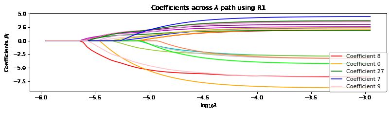
see Figure 2. Naturally, ground truth is not available for real data. However, Figure 4
highlights that naive sparse log-contrast estimation proposes different influential microbes
for the outcome than our two-stage ILR+LC. This indicates that the gut microbiome and
body weight may indeed be confounded. Therefore, under the IV assumptions, the ILR+LC
9 We note that recent non-linear IV methods such as Hartford et al. (2017); Bennett et al. (2019); Zhang et al.
(2020) cannot overcome the issues of 2SLS in this setting.
1110
4000 10
5
OOS MSE
5
3000 0
0
2000 −5
−5
1000 −10
−10
0 −15
ILR+LC KIVILR Only LC ILR+LC Only LC ILR+LC Only LC
Figure 3: The boxplots below summarize the results for setting B in Table 2 with p = 250, q =
10. We collected the OOS MSE (left) as well as the non-zero β components (middle) and
the zero β components (right). Only LC has troubles detecting non-zero components on
average due to the lack of causal interpretation. All results and visualizations can be found
in Appendix F.
CandidatusArthr
Phylum Influential Compositions
Tenericutes
Only LC
Verrucomicrobia
Tep
s
Bacteroidetes ILR+LC
Anaero
occu
Clostridium
idim
cus
De
Actinobacteria
ha
n
inoc
icrob -4
3
omitus
u
Proteobacteria
lob
riv pira
SMB5
Os erotr
St
vorax
re
ac
Rum
Firmicutes
rio
La
s
ium
rc4
us
pt
Bu illo
ter us
a
ct
ib
oc
cc
An
En o
c
ium
ter bac o
oc
oc
ty
c
An
ae
oc
o llu
i pr
rob ccu s Co rea
Geo
ac
ill
s Do utia c cu
s]
bac us Bla inoco
Staph i llus m
yloco [Ru
ccus buria
Rose
Turicibacte es
r Anaerostip
[Eubacterium] Robinsoniella
llus Anaeropla
Coprobaci sma
Akke
b a c ulum rman
Allo ium
Clo
acib
sia
strid ed Eli acte
Clo fi Pr abe
z rium
ssi a
n cla siell r O evo thkin
. | u b e do tel gia
En
t
Kl
e ct rib la
ba
Ad ob
na r
te
ac
ti ro
s
Bifi yneba
ac
le
te
Co
hold a
rc
ob
eria
Brac
C r
e
d
Actino
rium
mo
Sphingomonas
Saccharopolyspo
re
ora
r
et
ut
in
do
ac
zia
nd
hyba
Ac
obacte
eu
ter
Pa
myces
Burk
Ps
ium
c teri
cter
Janthin
um
ium
ra
Figure 4: Taxonomic tree of the microbiome data at genus level. The influential log-ratios
for both Only Second LC (black) and ILR+LC (blue) are disjoint.
12estimates carry causal meaning for individual abundances, whereas direct log-contrast
estimation solely surfaces correlation.
Discussion. Our results show that accounting for both the compositional nature as well
as confounding is not optional for cause-effect estimation with compositional causes. Our
two-stage methods not only reliably recover causal effects (OOS MSE), but also yield inter-
pretable effect estimates for individual abundances (β-MSE, FZ, FNZ) whenever applicable.
In particular, ILR+LC works reliably for non-sparse and sparse linear settings. When lin-
earity cannot be assumed or interpretable estimates for individual components of β are
not required, KIVILR can still perform well under these relaxed assumptions albeit being
challenging to tune for large p and unable to incorporate sparsity. While DIR+LC in theory
yields interpretable estimates and respects compositionality in both stages, our results high-
light the danger of the “forbidden regression” with DIR+LC and we cannot recommend this
seemingly superior method unless the data X are known to follow a Dirichlet distribution.
ILR+LC appears to be largely unaffected by first stage misspecification.
5 Conclusion
The compositional nature of many scientific datasets poses major challenges to statistical
analysis and interpretation—individual components are inherently entangled. Moreover,
the analyst is often faced with a large number of possible components with the difficulty
of identifying a parsimonious sub-composition of interest and has to deal with potential
unobserved confounding. Given the potentially profound impact of the microbiome on
human health or species abundances on global health, it is of vital importance that we
face these challenges and develop interpretable methods to obtain causal insights from
compositional data.
In this work, we developed and analyzed methods for cause-effect estimation with com-
positional causes under unobserved confounding in instrumental variable settings. As
we aim for informing consequential decisions such as medical treatments, we focused on
interpretability with respect to potential interventions. First, we crisply formulated the
limitations of replacing compositions with information theoretic summary statistics using
microbial diversity as a hall mark example.
Next, leveraging isometries to Euclidean space (e.g., ilr), we developed a range of methods for
cause-effect estimation and provided an in-depth analysis of how IV assumptions (including
misspecification or weak instrument bias) interact with compositionality. Neither can be
ignored. We evaluated the efficacy and robustness of our methods in simulation and on
real microbiome data. ILR+LC is particularly promising to provide interpretable and
theoretically sound answers to causal queries involving compositional causes from purely
observational data. Other seemingly well-suited methods such as DIR+LC fail, arguably
due to an interaction of misspecification and the compositional nature of the data. We hope
that we opened up avenues for future work on how to properly extend the causal inference
toolbox to compositional causes as well as effects.
Acknowledgments
We thank Dr. Chan Wang and Dr. Huilin Li, NYU Langone Medical Center, for kindly
providing the pre-processed murine amplicon and associated phenotype data used in this
study. We thank Léo Simpson, TU München, and Alice Sommer, LMU München, for kindly
and patiently providing their technical and scientific support as well as Johannes Ostner
for his excellent guidance on microbiome visualization techniques. EA is supported by the
13Helmholtz Association under the joint research school “Munich School for Data Science -
MUDS”.
References
Aitchison, J. The statistical analysis of compositional data. Journal of the Royal Statistical
Society: Series B (Methodological), 44(2):139–160, 1982.
Aitchison, J. and Bacon-Shone, J. Log contrast models for experiments with mixtures.
Biometrika, 71(2):323–330, 1984. ISSN 00063444. doi: 10.1093/biomet/71.2.323.
Andrews, I., Stock, J. H., and Sun, L. Weak instruments in instrumental variables regression:
Theory and practice. Annual Review of Economics, 11:727–753, 2019.
Angrist, J. D. and Pischke, J.-S. Mostly harmless econometrics: An empiricist’s companion.
Princeton university press, 2008.
Arnold, K. F., Berrie, L., Tennant, P. W., and Gilthorpe, M. S. A causal inference perspective on
the analysis of compositional data. International journal of epidemiology, 49(4):1307–1313,
2020.
Bello, M. G. D., Knight, R., Gilbert, J. A., and Blaser, M. J. Preserving microbial diversity.
Science, 2018. ISSN 0036-8075. doi: 10.1126/science.aau8816.
Bennett, A., Kallus, N., and Schnabel, T. Deep generalized method of moments for instru-
mental variable analysis. In Wallach, H., Larochelle, H., Beygelzimer, A., d'Alché-Buc,
F., Fox, E., and Garnett, R. (eds.), Advances in Neural Information Processing Systems, vol-
ume 32. Curran Associates, Inc., 2019. URL https://proceedings.neurips.cc/paper/
2019/file/15d185eaa7c954e77f5343d941e25fbd-Paper.pdf.
Blaser, M. J. Missing Microbes: How the Overuse of Antitbiotics Is Fueling Our Modern Plagues.
Henry Holt and Company, New York, first edit edition, 2014.
Blei, D. M. and Lafferty, J. D. Correlated topic models. Advances in Neural Information
Processing Systems, pp. 147–154, 2005. ISSN 10495258.
Blei, D. M. and Lafferty, J. D. A correlated topic model of Science. The Annals of Applied
Statistics, 1(1):17–35, 2007. ISSN 1932-6157. doi: 10.1214/07-aoas114.
Blundell, R., Chen, X., and Kristensen, D. Semi-nonparametric iv estimation of shape-
invariant engel curves. Econometrica, 75(6):1613–1669, 2007.
Bonet, B. Instrumentality tests revisited. In Proceedings of the 17th Conference on Uncertainty
in Artificial Intelligence, pp. 48–55, 2001.
Bradbury, J., Frostig, R., Hawkins, P., Johnson, M. J., Leary, C., Maclaurin, D., Necula,
G., Paszke, A., VanderPlas, J., Wanderman-Milne, S., and Zhang, Q. JAX: Composable
transformations of Python+NumPy programs, 2018.
Breskin, A. and Murray, E. J. Commentary: Compositional data call for complex interven-
tions. International Journal of Epidemiology, 49(4):1314–1315, 2020.
Cammarota, G., Ianiro, G., Ahern, A., Carbone, C., Temko, A., Claesson, M. J., Gasbarrini,
A., and Tortora, G. Gut microbiome, big data and machine learning to promote precision
medicine for cancer. Nature Reviews Gastroenterology and Hepatology, 17(10):635–648,
2020. ISSN 17595053. doi: 10.1038/s41575-020-0327-3. URL http://dx.doi.org/10.
1038/s41575-020-0327-3.
14Chao, A., Chiu, C.-H., and Jost, L. Unifying species diversity, phylogenetic diversity, func-
tional diversity, and related similarity and differentiation measures through hill numbers.
Annual review of ecology, evolution, and systematics, 45:297–324, 2014.
Chapin, F. S., Zavaleta, E. S., Eviner, V. T., Naylor, R. L., Vitousek, P. M., Reynolds, H. L.,
Hooper, D. U., Lavorel, S., Sala, O. E., Hobbie, S. E., Mack, M. C., and Díaz, S. Consequences
of changing biodiversity. Nature, 405(6783):234–242, 2000. ISSN 00280836. doi: 10.1038/
35012241.
Cho, I. and Blaser, M. J. The human microbiome: at the interface of health and disease.
Nature Reviews Genetics, 13(4):260–270, 2012.
Cho, I., Yamanishi, S., Cox, L., Methé, B. a., Zavadil, J., Li, K., Gao, Z., Mahana, D., Raju,
K., Teitler, I., Li, H., Alekseyenko, A. V., and Blaser, M. J. Antibiotics in early life alter
the murine colonic microbiome and adiposity. Nature, 488(7413):621–626, 2012. ISSN
0028-0836. doi: 10.1038/nature11400.
Clemente, J. C., Ursell, L. K., Parfrey, L. W., and Knight, R. The impact of the gut microbiota
on human health: an integrative view. Cell, 148(6):1258–1270, 2012.
Combettes, P. and Müller, C. Regression models for compositional data: General log-contrast
formulations, proximal optimization, and microbiome data applications. Statistics in
Biosciences, 06 2020. doi: 10.1007/s12561-020-09283-2.
Daly, A. J., Baetens, J. M., and De Baets, B. Ecological diversity: measuring the unmeasurable.
Mathematics, 6(7):119, 2018.
Egozcue, J. J., Pawlowsky-Glahn, V., Mateu-Figueras, G., and Barcelo-Vidal, C. Isometric
logratio transformations for compositional data analysis. Mathematical Geology, 35(3):
279–300, 2003.
Gautier, L., 2021. URL https://rpy2.github.io/.
Gloor, G. B., Macklaim, J. M., Pawlowsky-Glahn, V., and Egozcue, J. J. Microbiome datasets
are compositional: and this is not optional. Frontiers in microbiology, 8:2224, 2017.
Greenacre, M. and Grunsky, E. The isometric logratio transformation in compositional data
analysis: a practical evaluation. preprint, 2019. URL https://ideas.repec.org/p/upf/
upfgen/1627.html.
Greene, W. H. Accounting for excess zeros and sample selection in poisson and negative
binomial regression models. NYU working paper no. EC-94-10, 1994.
Gunsilius, F. Testability of instrument validity under continuous endogenous variables.
arXiv preprint arXiv:1806.09517, 2018.
Harris, C. R., Millman, K. J., van der Walt, S. J., Gommers, R., Virtanen, P., Cournapeau, D.,
Wieser, E., Taylor, J., Berg, S., Smith, N. J., Kern, R., Picus, M., Hoyer, S., van Kerkwijk,
M. H., Brett, M., Haldane, A., del Río, J. F., Wiebe, M., Peterson, P., Gérard-Marchant, P.,
Sheppard, K., Reddy, T., Weckesser, W., Abbasi, H., Gohlke, C., and Oliphant, T. E. Array
programming with NumPy. Nature, 2020.
Hartford, J., Lewis, G., Leyton-Brown, K., and Taddy, M. Deep iv: A flexible approach for
counterfactual prediction. In International Conference on Machine Learning, pp. 1414–1423,
2017.
15Hernán, M. A. and Robins, J. M. Instruments for causal inference: an epidemiologist’s
dream? Epidemiology, pp. 360–372, 2006.
Hunter, J. D. Matplotlib: A 2D graphics environment. Computing in Science & Engineering,
2007.
Imbens, G. W. and Rubin, D. B. Causal inference in statistics, social, and biomedical sciences.
Cambridge University Press, 2015.
Inc., P. T. Collaborative data science, 2015. URL https://plot.ly.
Kaul, A., Mandal, S., Davidov, O., and Peddada, S. D. Analysis of microbiome data in the
presence of excess zeros. Frontiers in microbiology, 8:2114, 2017.
Kelejian, H. H. Two-stage least squares and econometric systems linear in parameters but
nonlinear in the endogenous variables. Journal of the American Statistical Association, 66
(334):373–374, 1971.
Kilbertus, N., Kusner, M. J., and Silva, R. A class of algorithms for general instrumental
variable models. In Advances in Neural Information Processing Systems, volume 33, 2020.
Kurtz, Z. D., Bonneau, R., and Müller, C. L. Disentangling microbial associations from
hidden environmental and technical factors via latent graphical models. bioRxiv, 2019.
doi: 10.1101/2019.12.21.885889.
Leinster, T. and Cobbold, C. Measuring diversity: The importance of species similarity.
Ecology, 93:477–89, 03 2012. doi: 10.2307/23143936.
Lin, H. and Peddada, S. D. Analysis of microbial compositions: a review of normalization
and differential abundance analysis. NPJ biofilms and microbiomes, 6(1):1–13, 2020.
Lin, W., Shi, P., Feng, R., and Li, H. Variable selection in regression with compositional
covariates. Biometrika, 101(4):785–797, 2014. ISSN 14643510. doi: 10.1093/biomet/
asu031.
Lynch, S. V. and Pedersen, O. The human intestinal microbiome in health and disease. New
England Journal of Medicine, 375(24):2369–2379, 2016.
Mahana, D., Trent, C. M., Kurtz, Z. D., Bokulich, N. A., Battaglia, T., Chung, J., Müller,
C. L., Li, H., Bonneau, R. A., and Blaser, M. J. Antibiotic perturbation of the murine
gut microbiome enhances the adiposity, insulin resistance, and liver disease associated
with high-fat diet. Genome Medicine, 8(1):1–20, 2016. ISSN 1756994X. doi: 10.1186/
s13073-016-0297-9. URL http://dx.doi.org/10.1186/s13073-016-0297-9.
Muandet, K., Mehrjou, A., Lee, S. K., and Raj, A. Dual instrumental variable regression.
arXiv preprint arXiv:1910.12358, 2019.
Newey, W. K. and Powell, J. L. Instrumental variable estimation of nonparametric models.
Econometrica, 71(5):1565–1578, 2003.
Oh, M. and Zhang, L. Deepmicro: deep representation learning for disease prediction based
on microbiome data. Scientific Reports, 10, 04 2020. doi: 10.1038/s41598-020-63159-5.
Oksanen, J., Blanchet, F. G., Friendly, M., Kindt, R., Legendre, P., McGlinn, D., Minchin, P. R.,
O’Hara, R. B., Simpson, G. L., Solymos, P., Stevens, M. H. H., Szoecs, E., and Wagner, H.
vegan: Community Ecology Package, 2020. URL https://CRAN.R-project.org/package=
vegan. R package version 2.5-7.
16pandas development team, T. pandas-dev/pandas: Pandas, February 2020. URL https:
//doi.org/10.5281/zenodo.3509134.
Patuzzi, I., Baruzzo, G., Losasso, C., Ricci, A., and Di Camillo, B. metasparsim: a 16s rrna
gene sequencing count data simulator. BMC Bioinformatics, 20, 11 2019. doi: 10.1186/
s12859-019-2882-6.
Pawlowsky-Glahn, V. and Egozcue, J. J. Geometric approach to statistical analysis on the
simplex. Stochastic Environmental Research and Risk Assessment, 15(5):384–398, 2001.
Pearl, J. On the testability of causal models with latent and instrumental variables. In
Proceedings of the Eleventh conference on Uncertainty in artificial intelligence, pp. 435–443.
Morgan Kaufmann Publishers Inc., 1995.
Pearl, J. Causality. Cambridge university press, 2009.
Pedregosa, F., Varoquaux, G., Gramfort, A., Michel, V., Thirion, B., Grisel, O., Blondel,
M., Prettenhofer, P., Weiss, R., Dubourg, V., Vanderplas, J., Passos, A., Cournapeau, D.,
Brucher, M., Perrot, M., and Duchesnay, É. Scikit-learn: Machine learning in Python.
JMLR, 2011.
Pflughoeft, K. J. and Versalovic, J. Human microbiome in health and disease. Annual Review
of Pathology: Mechanisms of Disease, 7:99–122, 2012.
Quinn, T. P., Erb, I., Richardson, M. F., and Crowley, T. M. Understanding sequencing
data as compositions: an outlook and review. Bioinformatics, 34(March):2870–2878, 2018.
ISSN 1367-4803. doi: 10.1093/bioinformatics/bty175. URL https://academic.oup.com/
bioinformatics/advance-article/doi/10.1093/bioinformatics/bty175/4956011.
Quinn, T. P., Nguyen, D., Rana, S., Gupta, S., and Venkatesh, S. DeepCoDA: personalized
interpretability for compositional health data. arXiv, 2020.
R Core Team. R: A Language and Environment for Statistical Computing. R Foundation for
Statistical Computing, Vienna, Austria, 2020. URL https://www.R-project.org/.
Rivera-Pinto, J., Egozcue, J. J., Pawlowsky-Glahn, V., Paredes, R., Noguera-Julian, M., and
Calle, M. L. Balances: a new perspective for microbiome analysis. MSystems, 3(4):e00053–
18, 2018.
Rozenblatt-Rosen, O., Stubbington, M. J., Regev, A., and Teichmann, S. A. The human cell
atlas: from vision to reality. Nature News, 550(7677):451, 2017.
Rubin, D., Imbens, G., and Angrist, J. Identification of causal effects using instrumental
variables: Rejoinder. Journal of the American Statistical Association, 91, 07 1993. doi:
10.2307/2291629.
Sanderson, E. and Windmeijer, F. A weak instrument f-test in linear iv models with multiple
endogenous variables. Journal of Econometrics, 190(2):212–221, 2016. ISSN 0304-4076.
doi: https://doi.org/10.1016/j.jeconom.2015.06.004. URL https://www.sciencedirect.
com/science/article/pii/S0304407615001736. Endogeneity Problems in Economet-
rics.
Schulfer, A., Schluter, J., Zhang, Y., Brown, Q., Pathmasiri, W., McRitchie, S., Sumner, S., Li,
H., Xavier, J., and Blaser, M. The impact of early-life sub-therapeutic antibiotic treatment
(stat) on excessive weight is robust despite transfer of intestinal microbes. The ISME
Journal, 13:1, 01 2019. doi: 10.1038/s41396-019-0349-4.
17scikit-bio development team, T. scikit-bio: A bioinformatics library for data scientists,
students, and developers, 2020. URL http://scikit-bio.org.
Seabold, S. and Perktold, J. statsmodels: Econometric and statistical modeling with python.
In 9th Python in Science Conference, 2010.
Sender, R., Fuchs, S., and Milo, R. Revised estimates for the number of human and bacteria
cells in the body. PLoS biology, 14(8):e1002533, 2016.
Shade, A. Diversity is the question, not the answer. The ISME journal, 11(1):1–6, 2017.
Shreiner, A. B., Kao, J. Y., and Young, V. B. The gut microbiome in health and in disease.
Current opinion in gastroenterology, 31(1):69, 2015.
Simpson, L., Combettes, P., and Müller, C. c-lasso - a python package for constrained sparse
and robust regression and classification. Journal of Open Source Software, 6:2844, 01 2021.
doi: 10.21105/joss.02844.
Singh, R., Sahani, M., and Gretton, A. Kernel instrumental variable regression. In Advances
in Neural Information Processing Systems, pp. 4593–4605, 2019.
Sohn, M. B. and Li, H. Compositional mediation analysis for microbiome studies. Annals of
Applied Statistics, 13(1):661–681, 2019. ISSN 19417330. doi: 10.1214/18-AOAS1210.
Suh, E. J., 2020. URL https://github.com/ericsuh/dirichlet.
Tsagris, M. and Athineou, G. Compositional: Compositional Data Analysis, 2021. URL
https://CRAN.R-project.org/package=Compositional. R package version 4.5.
Turnbaugh, P. J., Ley, R. E., Hamady, M., Fraser-Liggett, C. M., Knight, R., and Gordon, J. I.
The human microbiome project. Nature, 449(7164):804–810, 2007.
van Rossum, G. and Drake, F. L. Python 3 Reference Manual. CreateSpace, 2009.
Vujkovic-Cvijin, I., Sklar, J., Jiang, L., Natarajan, L., Knight, R., and Belkaid,
Y. Host variables confound gut microbiota studies of human disease. Nature
2020, pp. 1–7, 2020. ISSN 0028-0836. doi: 10.1038/s41586-020-2881-9. URL
http://www.nature.com/articles/s41586-020-2881-9{%}0Ahttps://www.nature.
com/articles/s41586-020-2881-9?s=09.
Wang, C., Hu, J., Blaser, M. J., Li, H., and Birol, I. Estimating and testing the microbial causal
mediation effect with high-dimensional and compositional microbiome data. Bioinformat-
ics, 2020. ISSN 14602059. doi: 10.1093/bioinformatics/btz565.
Wes McKinney. Data Structures for Statistical Computing in Python. In Stéfan van der Walt
and Jarrod Millman (eds.), Proceedings of the 9th Python in Science Conference, pp. 56 – 61,
2010. doi: 10.25080/Majora-92bf1922-00a.
Willis, A. Rarefaction, alpha diversity, and statistics. Frontiers in Microbiology, 10:2407, 10
2019. doi: 10.3389/fmicb.2019.02407.
Xu, L., Paterson, A. D., Turpin, W., and Xu, W. Assessment and selection of competing
models for zero-inflated microbiome data. PloS one, 10(7):e0129606, 2015.
Zhang, R., Imaizumi, M., Schölkopf, B., and Muandet, K. Maximum moment restriction for
instrumental variable regression. arXiv preprint arXiv:2010.07684, 2020.
18You can also read