When We Change the Clock, Does the Clock Change Us?
←
→
Page content transcription
If your browser does not render page correctly, please read the page content below
Energy Institute WP 335

When We Change the Clock, Does the Clock Change Us?

   Patrick Baylis, Severin Borenstein, and Edward Rubin

                                     March 2023

Energy Institute at Haas working papers are circulated for discussion and comment purposes.
They have not been peer-reviewed or been subject to review by any editorial board. The Energy
Institute acknowledges the generous support it has received from the organizations and
individuals listed at https://haas.berkeley.edu/energy-institute/about/funders/.

© 2023 by Patrick Baylis, Severin Borenstein, and Edward Rubin. All rights reserved. Short
sections of text, not to exceed two paragraphs, may be quoted without explicit permission
provided that full credit is given to the source.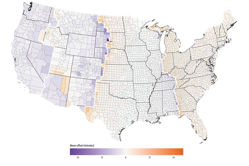
When we change the clock, does the clock change us?
                       Patrick Baylis, Severin Borenstein, and Edward Rubin *
                                                    March 3, 2023

                                                          Abstract

          Standardized time is a central device for coordinating activities and economic behavior across
       individuals. Time zones synchronize activities across large geographic areas, while daylight saving
       time coordinates a shift in clocks across a society, originally with the intent of reducing energy usage.
       However, there is nearly always conflict between an individual’s goals of coordinating activities with
       others and engaging in those activities at their own preferred time. When time is standardized across
       large geographic areas, that tension is enhanced, because norms about the “clock times” of activities
       conflict with adapting to local environmental conditions created by natural or “solar” time. This tension
       is at the heart of current state and national debates about adopting daylight saving time or switching
       time zones.
          We study this conflict by examining how geographic and temporal variation in solar time affects
       the timing of a range of common behaviors in the United States. Specifically, we estimate the degree
       to which people shift their online behavior (through Twitter), their commute (using data from the
      Census), and their visits to businesses and other establishments (using foot traffic data). We find that,
       on average, a one-hour shift in the differential between solar time and clock time—approximately the
      width of a time zone—leads to shifting the clock time of behavior by between 9 and 26 minutes. This
       result shows that while adapting to local environmental factors significantly offsets the differential
       between solar time and clock time, the behavioral nudge and coordination value of clock time has the
       larger influence on activity. We also examine how this trade-off differs across different activities and
       population demographics.

    * Baylis: Vancouver School of Economics, University of British Columbia, patrick.baylis@ubc.ca; Borenstein: Haas School of
Business and Energy Institute at Haas, University of California, Berkeley, severinborenstein@berkeley.edu; Rubin: Department of
Economics, University of Oregon, edwardr@uoregon.edu. For excellent research assistance, we thank Sara Johns.

                                                              1
2

1    Introduction
Coordinating the timing of activities with other people is a fundamental characteristic of society. But it’s
also a hassle. Individuals face different constraints and have different preferences about when activities
take place, so there is a constant tradeoff between coordinating with others and engaging in an activity
when one personally prefers. In a modern society with instantaneous long-distance communication and
high-speed travel, differences in environmental drivers of activity times – such as sunrise, sunset and
temperature – exacerbate the tension between coordination and personal preferences or environmental
constraints.

Technological advances in the U.S. during the 19th century, such as the adoption of the telegraph and
telephone, and the completion of the transcontinental railroad, increased pressure to coordinate the
denomination of time, so-called “clock time,” across locations. Prior to the 1880s, most towns in the
US operated on their own local clock times, based on “solar time” at their location, with noon occurring
when the sun was at its highest point. In 1886, the US became the first country to standardize clock
time across large regions, known as time zones. The change was driven, and first implemented, by the
railroads, who argued the previously existing system made scheduling trains across locations impossibly
complex (Prerau 2009).

Expectations of activities occurring at certain clock times permeate society, whether “bankers’ hours”
(9-to-3) or a standard workday (9-to-5) or lunch time (around noon). Recognizing the behavioral power
of clock time, in the early 20th century many governments instituted “daylight saving time”, an idea
suggested more than a century earlier by Benjamin Franklin. Since time zones were created, they have be-
come a device for coordinating activities across great distances. Beyond easing transportation scheduling,
time zones made it possible to synchronize the timing of activities that occur across large geographies,
such as telegraph and telephone communication, and radio and television broadcasting.

Clock time is a purely nominal metric, so in theory, a change in the metric that preserves the corre-
spondence to elapsed time need not have any impact on behavior, regardless of how it synchronizes
with solar time. Yet, such changes – in the form of time zones and daylight saving time – do seem to
affect behavior in practice, possibly because individuals anticipate that others will change their behavior
and wish to coordinate on when activities occur (Barnes and Wagner 2009; Gibson and Shrader 2018;
Giuntella and Mazzonna 2019; Hamermesh, Myers, and Pocock 2008). When such coordination occurs
across distant locations, however, it is more likely to move the timing of activities away from the choices
people would make based purely on solar time.

Fundamentally, standardizing the time of activities across longitudes means that they take place earlier
(in solar time) in locations that are further west. If there is an optimal solar time to awaken, eat meals,
or begin the work day, one wouldn’t expect it to be the same clock time in Portsmouth, New Hampshire
as in Grand Rapids, Michigan. Both cities are in the Eastern time zone, but the sun rises about one hour
later in Grand Rapids. Thus, in order to understand how changing the denomination of time might alter
behavior in the long run, a useful starting point would be to understand how behavior differs among
people living under the same clock time, but different solar times. To what extent do their activities
take place at the same clock time – due to widespread social norms, the desire to coordinate activities
3

across locations, or other factors – and to what extent do they adapt to local solar time at the expense
of coordination or norms?

We study this trade-off using three different datasets that focus on different behavior and have been
collected in different ways. First, we examine data from Twitter, focusing on when individuals send
out tweets. Second, we use data from the 2000 U.S. Census longform in response to a question asking
when individuals leave for work. And third, we study aggregated, cellphone-based foot-traffic data from
Safegraph on the timing of visits to retail establishments. In all three cases, we use the data to ask
when certain behaviors take place as a function of local clock time and solar time. More simply, we ask
whether, within a time zone, specific behaviors take place later (according to clock time) among people
who are further west, which has a later solar time.

We control for many potential confounders in the analysis, including latitude, population density, employ-
ment types, age demographics and household compositions. One issue not captured by those covariates,
however, is connectedness between locations. Nashville, TN, for instance, is in the Central time zone, but
not far from Knoxville, TN, which is in the Eastern time zone. One would worry that a simple analysis of
when activities occur might conflate the impact of solar time (relative to a location’s clock time) with the
impact of coordinating with other locations that are potentially in a different time zone. If two locations
have the same solar time and clock time, but the individuals in one location have stronger ties to people
in another time zone, then that connectedness might change their behavior.

We capture this effect with a connectedness index we have created from anonymized cellphone data
that measures the tendency of a phone detected in one specific county to also be detected in another
specific county. We have also carried out the analysis using two other measures of connectedness
between locations: (1) the Social Connectedness Index created by Bailey et al. (2018), based on “friends”
connections across counties on Facebook and (2) a gravity model, hypothesizing that the influence of
other counties will vary with their distance from the observed county and their population or economic
size. We find that the new index based on cell phone locations has greater explanatory power, but the
effect of solar time is not substantially changed by its inclusion.

The value of coordination across locations also likely differs depending on the activities that an individual
is engaging in on a given day. So, for instance, leisure time might create different trade-offs between
coordination and responding to local environmental factors than work time. Similarly, work or leisure
activities taking place outdoors likely create different trade-offs than those occurring indoors. We
incorporate these varying trade-offs by differentiating between weekend and weekday activities, as well
as between workers in outdoor-oriented versus indoor-oriented occupations. 1

A small body of literature examines the relationship between time and economic behavior. Empirical
investigations into the relationship between time of day and human activity generally fall into two
categories: those that examine the effects of Daylight Saving Time and those that examine how sleep,
driven by sunrise time, impacts productivity.

In the area of environmental and energy economics, the impact of clock time has been examined by
   1. It is also worth pointing out that technological progress in the last decade may be changing the value of coordination. The
increasing availability of on-demand entertainment and technologies that accommodate more effective work from home may
reduce the cost of unsynchronized leisure and work times.
4

studying the effect of Daylight Saving Time (DST) on energy use, and more generally the possibility
of reducing energy use by changing the denomination of time. Those studies have focused on the
outcome variable – net change in energy use – but have not directly confronted the larger question of
the mechanism by which the denomination of time affects behavior. It is possible that re-denomination
does change behavior, but the net impact on energy use is still near zero, as suggested by these studies,
or that the re-denomination does not change behavior much at all.

In general, although DST was putatively designed to save energy, the evidence on that front is mixed at
best. Kellogg and Wolff (2008) conclude that DST extension in some Australian states to accommodate
the 2000 Sydney Olympics did not lead to a net change in electricity consumption, only that it shifted the
time of consumption. Kotchen and Grant (2011), examining household bills in Indiana, find instead that
energy usage actually increases as a result of DST. By contrast, Rivers (2018) concludes that electricity
demand decreases following the start of DST in Ontario. Shaffer (2019) provides some evidence to
reconcile the disparate results in the literature: he investigates consumption across Canadian provinces
and finds that places with later sunrises, i.e., those located farther west in a time zone, are more likely
to experience energy use increases as a result of DST. Other work on DST examines its safety impacts:
Barnes and Wagner (2009) look at sleep losses following the DST changeovers and find that mine
accidents tend to increase following the “loss” of an hour due to the “spring forward” adjustment, while
Smith (2016) suggests that an increase in fatal vehicle crashes following the spring DST change is due
to the loss of sleep, not the shift in light. Doleac and Sanders (2015) find that the additional daylight in
evening clock hours due to DST reduces crime.

The other category of studies instead uses geographically driven differences in sunset time to document
the negative effects of sleep on productivity or performance in the classroom. Heissel and Norris (2018)
instrument hours of sleep with sunrise time to show that more sleep leads to improvements in test scores
for adolescents. Gibson and Shrader (2018) similarly instrument sleep time with sunset time and find
that both short-run variation in sunset/sleep time and long-run, cross-sectional variation in sunset/sleep
time reduce earnings in the United States. In other words, living on the western edge of a time zone
reduces wages, all else equal. Using data from several developing countries, Jagnani (2018) concludes
that later sunset times reduce sleep, study effort, and eventually, educational outcomes. 2

In general, economic studies of time and behavior have uncovered several important relationships: DST
switches do not generally lead to significant electricity savings, and the timing of sunlight time can
alter safety, productivity, and even long-run earnings by disrupting sleep patterns. However, very few of
these studies have been able to examine the precise nature of the shifts in activity that underlie these
relationship. The sole exception of which we are aware is Hamermesh, Myers, and Pocock (2008).
Using time use data from Australia, they examine how sleep, work, and television viewing are altered
by sunlight time and the timing of network television.

Between 2020 and 2022, at least 33 states have considered legislation to change their use of daylight
saving time or to change their time zone, either of which also requires federal action. 3 Nearly all
proposals would abandon the semi-annual switch between standard and daylight saving time. In 2022,
  2. See also Giuntella and Mazzonna (2019) and Ingraham (2019).
  3. https://www.ncsl.org/transportation/daylight-saving-time-state-legislation
5

federal legislation to put all of the US on permanent daylight saving time passed the Senate, but died
in the House. 4 Policy debates over DST and changing time zones are very similar, because choosing
to live on standard time or DST is equivalent to choosing to adopt the clock time of one time zone or
an adjacent time zone. Debates over DST amount to debates over how much of the year a location
will choose to be in one time zone versus an adjacent time zone. Nearly all policy discussions of these
proposed changes, and most of the previous academic literature on these topics, have assumed that
individuals will continue to engage in activities at the same clock time regardless of how it synchronizes
with solar time. 5

It seems clear that the nudge of moving clock time away from solar time changes the timing of human
behavior to a significant extent, but it is not clear how much local environmental conditions restrain
that response. Assessing the potential impact of changing time conventions on energy use and human
activity requires a deeper understanding of how and how much departures of clock time from solar time
matter. We provide both a simple theoretical model of these tradeoffs and a detailed investigation of the
degree to which they do in three different large-scale datasets on human activity timing. This project is,
to our knowledge, the first study of the topic.

2      A Model of Coordination and Activity Timing
We illustrate the competing preferences of individuals through a simple model of two entities in locations
with different solar time but the same clock time. An entity could be a person, firm, or any other agent
that interacts with others in the world, but for this illustration we will discuss entities as people. If
the natural environment – e.g., light, temperature, humidity – were constant, then coordinating the
time of activities among people would be less likely to create systematic mismatches of preferences
between people in different locations. But because the natural environment changes at times that
differ systematically across locations, preferences among people for when activities occur will also differ
systematically across locations.

Assume that the utility that individual i gets from a specific activity is a declining function of the
deviation of the time of the activity from the individual’s own preferred time ti∗ and a declining function
of deviation from the time at which another individual, j, engages in the activity,

                                           Ui = U0i − fi (|ti − ti∗ |) − gi (|ti − t j |).

And likewise for individual j,
                                           U j = U0 j − f j (|t j − t∗j |) − g j (|ti − t j |).

We assume that f (0) = 0, f 0 () > 0 and f 00 () > 0, and g(0) = 0, g0 () > 0 and g00 () > 0 for both i and j. 6
Arbitrarily, assume that ti∗ < t∗j , so each individual will be engaging in the activity between t = ti∗ and
t = t∗j . Then, individual i’s best response to t j is determined by − fi0 + g0i = 0. Conversely, j’s best response
to i’s choice of ti is f j0 − g0j = 0. Under the assumptions on f (·) and g(·), this yields a best response function
    4. https://www.businessinsider.com/house-failed-vote-daylight-savings-time-permanent-sunshine-protection-act-2022-12
    5. See, for instance, Farrell, Narasiman, and Ward Jr. (2016) and Bokat-Lindell (2021).
    6. To assure an interior equilibrium, we also assume that fi0 > g0i and f j0 > g0j for all t.
6
ti∗ − t∗j
Best response for i
i’s activity-time deviation from t∗j
tie − t∗j
Best response for j
tej − ti∗ t∗j − ti∗
j’s activity-time deviation from ti∗
Figure 1: Best-response time choices and equilibrium timing of activities
for i that deviates further from ti∗ (i’s preferred time) the further is t j from ti∗ . Thus, if j engaged in the
activity at ti∗ , then i would also do so at ti∗ . And as j acts at a time further from ti∗ towards t∗j , i would
shift their activity time towards t∗j . Likewise, if i engaged in the activity at t∗j , then j would also do so at
t∗j , and as i acts at a time further from t∗j towards ti∗ , j would shift their activity time towards ti∗ .
Figure 1 illustrates the best responses of each individual and the unique equilibrium in which ti∗ < tie <
tej < t∗j . In the case illustrated here, j strongly prefers carrying out the activity near t∗j compared to the
value they get from carrying it out at a time near ti , while i gets a relatively higher value from more
coordinated timing.
An alternative model might constrain different individuals to act at the same time. For instance, a
third party might try to schedule a single time for an activity with these (and potentially many other)
individuals who have different preferred times of the event (and little or no private value of coordination)
– such as broadcasting a television show or setting standardized work hours for a multi-location firm.
The third party – such as the broadcaster or employer – is trying to minimize the schedule hassle costs
across all participants. In that case, the third party is trying to choose an activity time to minimize
min fi (|t − ti∗ |) + f j (|t − t∗j |).
t
Under the same regularity conditions, the optimal scheduling of the event occurs at ti∗ < topt < t∗j .
The model illustrates that, in equilibrium, activities will be influenced both by local factors that affect
individuals’ own preferred times for activities and by the value of coordinating activities across locations.
This implies that individuals at the east end of a time zone are likely to engage in activities earlier than
individuals at the west end of a time zone, measured in the same clock time. The relative weights on7
own preferred event time versus the value of coordination will determine how much activity times differ
across a time zone. To determine that, we turn to empirical analysis.
3 Data
To give some context to the data we utilize for the analyses, we first introduce a conceptual estimating
equation, variations of which we use in analyzing each of the three datasets.
None of the three datasets includes granular information on individuals engaging in the activity beyond
the time and location, so in each case we aggregate the data by time and location. We then can observe
the distribution of an activity over time of day for a given location.
Taking i as location and t as the observed day or week, our general empirical specification is:
Mean Activity Timeit = β ∗ Sunrise Timeit + δ ∗ Connectednessi + φT Z + Xit + εit (1)
Sunrise Timeit is the main variable of interest. For a given latitude on a given day, it indicates the extent
to which the solar time at location i on date t differs from clock time. Connectednessi controls for the
degree to which a location is connected to other areas with different clock times (explained in greater
detail below). φT Z is a set of time zone dummy variables that allow different baseline clock times for the
activity in different time zones, so they capture whether the activity on average occurs at different clock
times in different time zones. Xit is a vector of controls that includes latitude bins and time of year fixed
effects. 7
A positive β would indicate that the timing of the observed activity is responsive to solar time, not just
clock time. For instance, if eating lunch were the activity, β = 1 would indicate that people on the
western edge of a time zone eat lunch one hour later than people on the eastern edge of the time zone,
so clock time is the dominant driver for this activity. By contrast, β = 0 would indicate that the activity
follows clock time alone, ignoring solar time differences. β = 0.4 would indicate a partial adherence to
solar time, with people on the western edge of a time zone eating 0.4 hours (24 minutes) later than
people on the eastern edge on average, even though solar time is one hour later.
We modify this general equation to accommodate the different temporal frequencies and locations
available for each dataset, as well as to conduct a range of sensitivity tests.
The level of aggregation that represents an observation differs across the datasets. In the next three
subsections, we outline in more detail how this estimation is implemented with each of the three
datasets.
3.1 Twitter
We use data from the social media platform Twitter as one measure of activity timing across the United
States. To do so, we downloaded approximately 2.5 billion geolocated tweets through a connection to
7. It is possible that connection to locations within the same time zone, but with different solar time, could also affect quantity
of activity at a given location. None of our analysis, however, has found evidence of such an effect significantly changing behavior
timing.8
Twitter’s Streaming API. 8 For each date in our time period, which ranges from April 2014 to March 2019,
we compute both the average time of the tweets on that date and the average time for tweets containing
the following phrases: “breakfast”, “lunch”, “dinner”, “good morning”, and “good night”.
The pattern of tweet timing for each of our phrases is broadly consistent with expected times. Figure
2 documents the occurrence of each phrase throughout the day: “good morning” occurs earliest in the
day, followed by “breakfast”, “lunch”, “dinner” and “good night” (which actually has its peak in the early
morning hours).
0.4
0.3
Percent of tweets
0.2
0.1
0.0
0 4 8 12 16 20 24
Hour of day
Breakfast Lunch Dinner Good morning Good night
Figure 2: Twitter phrases by time of day
Across all tweets, activity peaks around the middle of the day. Because all of the tweets we download and
use are geolocated, we identify the county in which each tweet occurs. We then compute the average
time of tweets overall – as well as tweets with each activity phrase – by county and date. 9
8. These are the approximately 2% of public tweets from users who have permitted geolocation, so they are not a random
sample of tweets. Still, there’s no obvious reason that this would bias our estimation of the impact of clock time versus solar
time. A more comprehensive description of the methods by which we obtain, store, and process these data can be found in Baylis
(2020), though that paper also computes sentiment for each tweet, which we do not use here.
9. For the Twitter and census analysis, we measure the time of an activity in hours after 4 AM, because that is approximately
the minimum activity time in these data. We are in the process of making the same conversion for the foot traffic analysis, but
the data presented here use midnight as the start of each day. Using 4 AM minimizes concerns about whether a given activity is
occurring late on one day or very early on the following day. Measuring activity time in hours after midnight does not substantially
change the results, but does indicate some activity very early in days that is almost certainly actually part of activity from the
previous day.9 3.2 Census Census data contribute to our analysis based on questions about when the respondent leaves for and arrives at work. The 2000 census longform asked what time during the week prior to “Census Day” (which was April 1, 2000) the respondent typically left for work. 10 For each of slightly more than 200,000 census block groups, we use the average reported departure time as the primary variable of interest, but we also analyze the mean of arrival at work with nearly identical results. 11 Unlike the other two datasets we study, the census data have no time-series variation. They are simply a cross-section snapshot. In addition, the measures of departure time and travel time are self-reported, with all of the potential recall error issues that creates. Still, there is no clear reason that would bias our estimation of the impact of solar time on this activity. These data also have the potential advantage of being a 17% sampling of the entire population with extremely high response rates. 3.3 Foot traffic To analyze both the effects of time measurement on human mobility and the degree of connectedness between areas, we use cellphone-based foot-traffic data from SafeGraph (SafeGraph 2021b). These record data on visits to approximately 6.6 million points of interest (POIs) across the United States. SafeGraph defines a point of interest as any non-residential location a person can visit—ranging from restaurants and hardware stores to parks, post offices, and churches. These 6.6 million POIs cover 418 six-digit NAICS (North American Industry Classification System) codes during our sample period. We focus on visits during 2018 and 2019 due to that facts that (1) 2018 is the earliest year available and (2) data for 2020 and 2021 were distorted by COVID. For the main analyses, we focus on POIs that satisfy three sample-inclusion criteria: POIs (1) have at least one visit each week during 2018-2019 (excludes POIs that open or close in the middle of the sample), (2) have a median of at least 14 weekly visits, 12 and (3) are not missing location-related data. The resulting dataset includes 22.4 billion visits (91.6% of all visits in the dataset) to 2.2 million POIs covering 378 six-digit NAICS codes. 13 In raw form, this POI dataset 14 allows us to see the number of visits to a POI by hour of sample, for example, the number of visits to a specific Walmart between 8 AM and 9 AM on March 14, 2021. We also know each POI’s Census block group (CBG). We then collapse the dataset to POI by week-of-sample. For each POI-week, we calculate the average visit time and the average time of sunrise (based upon the POI’s CBG)—also summarizing each week’s activity by weekdays and weekends. 10. This was question 24 of the long form: 24(a) What time did this person usually leave home to go to work last week? and 24(b) How many minutes did it usually take this person to get from home to work last week? In 2000, daylight saving time began on April 2 in the United States. 11. Arrival time is calculated as the average departure time plus average travel time to work. 12. Because we weight regressions by the POI’s number of visits, the POIs omitted by this second requirement do not contribute very much to point estimates—but still require substantial computation. 13. Our main analyses omit all of Arizona because most of Arizona does not participate in daylight saving time. As Appendix Table 6 demonstrates, dropping Arizona does not affect our results. 14. We specifically use SafeGraph’s “weekly” POI dataset.
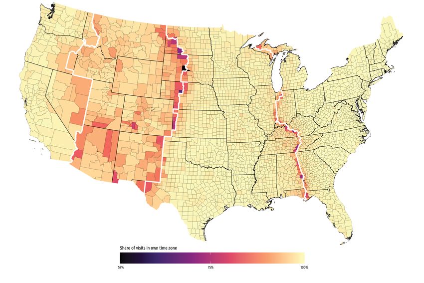
10

3.4     Controlling for connectedness
A potential source of confounding in a regression of activity time on solar time (controlling for time
zone) is that people in locations near the edge of a time zone border may be connected in some way to
locations in other time zones and may shift their activities in order to coordinate with the neighboring
time zone. For example, most of the Florida Panhandle west of Tallahassee is in the central time zone,
but the closest large city (and the state capital) is Tallahassee. Someone working in Panama City, Florida
(on the eastern edge of the Central time zone) may interact frequently with workers in Tallahassee. That
person may adjust their schedule, for example, by working 8-4 instead of 9-5 in order to synchronize
work time with Tallahassee. If locations near time zone borders are systematically more likely to link
to locations on the other side of that border, a regression without a connectedness control could find a
relationship between activity time and solar time even in the absence of a true causal effect.

To account for this possibility, we construct a set of variables that measure the proportion of observed
visits from residents of one time zone that occur in other time zones. For this calculation, we use a
second SafeGraph dataset that SafeGraph constructed to measure daily, Census block group (CBG)-level
social distancing. These data are available starting in 2019 (SafeGraph 2021a). This dataset records
v[hCBG , dCBG , t], the number of visits v to destination CBG dCBG from individuals who live in CBG hCBG at
time period t. We aggregate across time and within county. This aggregation produces a static, county-
level matrix with cells V[h, d]: the number of visits V from residents of county h to county d. To normalize
this measure (controlling for the population of h), we divide by the total visits generated by the residents
of h, i.e., V[h, •]. We define this ratio as county h’s connectedness to county d: C[h, d] = V[h, d]/V[h, •],
i.e., the share of visits from residents of county h to county d. 15

Counties with connections in time zones more to the east of their own will presumably be pulled
‘earlier’ (by clock time) into their days. To measure this ‘pull’, we use the county-level connectedness
C[h, d] measure to calculate the average time zone offset for each county—weighting each county’s
connectedness to the time zones by its connections to the time zones’ counties C[h, d]. For example,
If 60% of a county’s visits occur in its own time zone (where the time-zone difference is 0) and 40%
of visits occur in the adjoining time zone to the east (where the time-zone difference is 1 hour), then
we calculate the county’s mean time-zone offset is 0.4 hours. This measure effectively gives the visits-
weighted average clock-time difference. Appendix Table 4 summarizes this mean time-zone offset
variable—in addition to summarizing counties’ connectedness to each individual time zone and to their
own time zones. Unsurprisingly, the average county is very strongly connected to its own time zone
(with 97% of visits occuring in its own time zone), yielding a mean time-zone offset near zero. Appendix
Figures 5 and 6 illustrate the spatial distribution of these measures. As expected, connectedness to other
time zones is strongest for counties near time-zone boundaries.

We also have estimated the models with a “gravity” measure of connectedness— where the strength of
connection to another location is an inverse function of the distance to that location and a direct function
of the population mass at that location—and with the Social Connectedness Index developed in “Social
Connectedness: Measurement, Determinants, and Effects,” by Bailey et al. (2018) based on “friends”
connections across counties on Facebook. Neither of these variables appears to explain the measures of
 15. The vast majority of visits occur within individuals’ counties of residence, so C[h, h] is typically above 0.6.
11

activity time we study as well as the measure that we develop with cell phone data. Nonetheless, the
estimated effects of solar time on activity are reduced only slightly by inclusion of any connectedness
variable.

4     The effect of solar time on activity
4.1    Twitter
For the Twitter dataset, we estimate the model

              Mean(Tweet time)ct = β ∗ Sunrisect + δ ∗ Connectedness offsetc + φc + πt + εct

for county c on date t. Sunrise timect is determined by county centroid and date, Connectedness offsetc
is the average connectedness offset described in Section 3.4, φc are time zone by one-degree latitude bin
fixed effects, [Time zone × Lat. bin]c , and πt is a date-of-sample fixed effects. Mean(Tweet time)ct refers
to the average tweet time in that county-date for either all tweets in the dataset for that date-county, or,
in the next section, tweets containing a specific key phrase. We weight this regression by the average
count of tweets for the county, and cluster standard errors by state.

                          Table 1: Effect of sunrise time on tweet time

                                                            Avg. tweet time

                                                            (1)          (2)
                           Panel A: All days
                             Sunrise time                0.3571∗∗∗    0.3615∗∗∗
                                                         (0.0618)     (0.0982)
                              Avg. conn. offset                        0.2514
                                                                       (3.051)
                           Panel B: Weekdays
                             Sunrise time                0.3459∗∗∗    0.3613∗∗∗
                                                         (0.0647)     (0.1067)
                              Avg. conn. offset                        0.8766
                                                                       (3.393)
                           Panel C: Weekends
                             Sunrise time                0.3856∗∗∗    0.3621∗∗∗
                                                         (0.0569)     (0.0794)
                              Avg. conn. offset                         -1.346
                                                                       (2.264)
                            TZ×Lat. bin fixed effects        X            X
                            Date fixed effects               X            X
                          Notes: Observations are county by date. Standard errors
                          clustered by state.

The results in column (1) for all days indicate that tweets from people located at the west end of a time
12
zone on average occur about 0.36 hours (22 minutes) later in clock time than from people located at the
east end of a time zone, where the sun on average rises one hour earlier. In other words, for this activity
at least, people have adjusted their behavior by slightly more than one third of the solar time differential
between locations that have the same clock time. The effect is slightly larger on weekends than on
weekdays—consistent with the hypothesis that on weekends individuals are more inclined to adapt to
their local environment and less inclined to follow clock time—but the difference is not statistically
significant.
The results in column (2) indicate that connectedness of a county to locations in other time zones does
not significantly change when a person tweets. In fact, we would expect the sign of this coefficient to be
negative to the extent that greater connectedness with people in a "later" (further east) time zone would
cause one to engage in activities earlier as measured in local clock time. That is consistent with the point
estimate on weekends, but not the estimate on weekdays. Still, the coefficients are not estimated with
sufficient precision to draw any concrete conclusions.
4.2 Census
For the census data analysis, we have a single observation for each CBG indicating the average time at
which the respondents reported typically departing to go to work during the last week of March. As with
the Twitter data, we control for time zones by latitude, but we do not need to control for date because
this is a single cross-section.
Mean(departure time)c = β ∗ Sunrisec + δ ∗ Connectedness offsetc + φc + εc
for CBG c. Sunrise timec is determined for the CBG centroid on April 1, 2000. The other variables and
coefficients are as defined in the Twitter analysis. This equation does not include time fixed effects,
because the sample is a single cross-section. We weight this regression by the CBG population, and
cluster standard errors by state.
Table 2: Effect of sunrise time on time left for work
Time left for work
(1) (2)
∗∗∗
Sunrise time 0.3718 0.4285∗∗∗
(0.0538) (0.0570)
Avg. conn. offset 1.744∗∗
(0.8655)
N obs. 188,246 188,246
TZ × Lat. bin (1 deg.) fixed effects X X
Notes: Observations are CBGs. Excludes Indiana and Arizona. Standard errors clustered by state.
The results in column (1) are very consistent with the Twitter data results, indicating that people offset
clock time by slightly more than one-third of the difference between clock time and solar time. Column13
(2) suggests that connectedness has a statistically significant impact on activity time, but not with the
expected sign. The positive sign indicates, for instance, that greater connectedness with locations to the
east of one’s own time zone causes one to leave for work later in the day, measured by local clock time.
The effect, however, is estimated to be rather small and not very precisely estimated. A change in mean
offset connectedness from the 25th to 75th percentile value adjusts the departure time for work by 2.8
minutes with a 95% confidence interval of [0.15, 5.45] minutes.
4.3 Foot traffic
We estimate the model
Mean(Visit time)inw = β ∗ Sunrisecw + δ ∗ Connectedness offsetc + φc + πw + γnz + εinw
for POI i in 6-digit NAICS category n during week w. CBGs, c, determine longitude and latitude bins, as
well as the sunrise time during the observed week, w. Connectedness is determined by the county in
which the POI’s CBG is located, as with the analyses of Twitter and census data. This regression also in-
cludes fixed effects of NAICS code by time zone γnz . The Mean(Visit time) refers to the average visit time
to i during week w. We aggregate all days of the week and then break it out by weekday/weekend.
The results, presented in table 3, again show a statistically significant adaptation to solar time and away
from purely following clock time, but the effect estimated in this case is slightly less than half as large
as the results from the Twitter or census data. Including latitude bin by time zone fixed effects, the
top panel of column (1) suggests that people on the west end of a time zone frequent similar points of
interest about nine minutes later on average than people on the east end of the time zone. Somewhat
surprisingly, the effect is nearly the same on weekdays as on weekends.
As before, adding the connectedness variable does not change the impact of solar time by much at
all. For weekends, however, connectedness does have a statistically significant effect of the expected
negative sign, implying that stronger connectedness with people in a more easterly time zone causes
one to operate on an earlier schedule in local clock time. The effect, however, is still quite small. The
coefficient suggests that a change in mean offset connectedness from the 25th to 75th percentile value
adjusts the time of visiting a POI by 2.2 minutes.14
Table 3: Foot-traffic results: Effects of sunrise and connectedness on visit times
Avg. visit time
(1) (2)
Panel A: All days
Time of sunrise 0.1544∗∗∗ 0.1645∗∗∗
(0.0261) (0.0304)
Avg. conn. offset 0.4875
(0.8864)
N obs. (millions) 159.43 159.43
Panel B: Weekdays
Time of sunrise 0.1452∗∗∗ 0.1469∗∗∗
(0.0458) (0.0462)
Avg. conn. offset 0.0813
(1.042)
N obs. (millions) 159.40 159.40
Panel C: Weekends
Time of sunrise 0.1428∗∗∗ 0.1200∗∗∗
(0.0316) (0.0293)
Avg. conn. offset -1.108∗∗
(0.4405)
N obs. (millions) 155.08 155.08
Week-of-sample fixed effects X X
TZ × NAICS (6 digit) fixed effects X X
TZ × Lat. bin (1 deg.) fixed effects X X
Notes: An observation in this table is a POI-week, for example, a single Walmart during the week of 2021-03-14.
Column (2) controls for the county’s average offset (in minutes): More negative values of connectedness variable
imply a stronger connection to westward time zones. Clustered (state) standard-errors in parentheses. Significance
codes: ***: 0.01, **: 0.05, *: 0.1.15 5 Heterogeneity in Adaptation to Solar Time In the previous section, we presented average, pooled results for different types of activities controlling for only very basic heterogeneity: day, location, and connectedness to other locations. However, we have more detailed information about characteristics of the location and the observed activity. For each CBG, we know a number of demographic variables that could influence the degree of adaptation to solar time. In the Twitter dataset, we also have information from the content of the tweet. And in the foot traffic dataset, we know the line of business or activity associated with the POI. In general, one might expect that activities (or CBGs) more strongly linked to the outdoors would produce a stronger link to solar time. We now estimate the effect of solar time in separate regressions for the various demographic and activity categories, and report the estimated effect of sunrise on the timing of the activities. Figure 3 presents separate estimates on the effect of sunrise time, with the dataset split along different dimensions. The top panel shows results for areas north and south of the median population-weighted latitude in the continental US. For all three datasets the point estimate of the effect of solar time on the clock time at which the activity occurs suggests that people in locations further north adapt to local solar time more than people who live in the southern part of the country. The pattern is consistent in all three datasets, statistically significant at 5% level in the foot-traffic data, and statistically significant at 10% level in the Twitter and census datasets. One possible explanation is that people living further north are used to adjusting to large variations in sunrise, sunset and total sunlight time between the winter and summer, which makes time norms less rigid. As a result, they are more likely to also adjust to variations across longitude in the clock time of that sunlight. The next panel differentiates between summer and winter, where we do not see a consistent pattern or statistically significant differences. The following two panels attempt to get at outdoor activity. Rural areas are typically associated with living closer to nature, whether in line of work or choice of leisure activities. So we might expect that there is greater adaptation to solar time in rural than in urban locations. We see essentially no difference in analyzing the time of departure for work in the census data, but we do see a statistically significant difference in the foot-traffic dataset (and marginally significant differences in the Twitter data), suggesting that rural counties adapt more to solar time than do urban counties. That pattern, however, does not hold in the following panel where counties with larger shares of outdoor workers are, if anything, less likely to adapt to solar time. In the fifth panel, we compare locations by their share of population in the workforce (splitting at the median workforce share). Perhaps surprisingly, in all three datasets, counties with larger population shares in the workforce adapt more to solar time than counties with smaller shares; the differences are marginally significant in the foot-traffic and census datasets. The bottom panel of Figure 3 takes advantage of the content of the tweets in the Twitter data, looking in particular at tweets that include the words "breakfast", "lunch", "dinner", "good morning", or "good night". The estimated solar time adaptation for "good night" is positive, but is very imprecise, likely due to the extremely wide range of times it shows up in the dataset, including hours that we count as early
16

morning. The estimate for "good morning" is very much in line with overall adaptation at around 0.3.
All three meal reference estimates suggest adaptation to solar time, but breakfast seems to have by far
the largest adjustment, indicating that discussions of breakfast shift across the longitudes of a time zone
by nearly half of the shift in solar time.

Figure 4 uses only the foot traffic data and focuses on POIs in the 25 most common establishment
types, as indicated by six-digit NAICS code. The top nine types are all retail stores, and indicate a fairly
consistent pattern of adjustment to solar time with most estimates between 0.25 and 0.35, except for
auto parts and drugstores, which are around 0.1. Restaurants and hotels also are in the same general
range of adaptation.

Operations support services at airports—which includes airport retail outlets as well as entities providing
aircraft servicing and related operations—are not estimated to exhibit as much adaptation to solar time,
though the estimate is not very precise.

Among the other categories, the lack of adaptation at religious establishments (primarily churches,
temples and mosques), colleges and universities, medical care, and child daycare are noteworthy. Also
interesting, the fitness and outdoor categories are estimated to adapt to solar time, but no more so than
the retail categories.
17

Figure 3: Coefficient heterogeneity by demographic, geographic, and temporal subsets

           North

            South

         Summer

           Winter

            Rural

           Urban

           Indoor

         Outdoor

     Nonworking

        Working

        Breakfast
           Lunch
          Dinner

                    -0.5                               0.0                                    0.5

                                       Estimated coeffcient: Effect of sunrise on mean activity time

                                            Dataset:         Census       Twitter       POI

Notes: Each point-segment pair presents a coefficient and its 95% confidence interval from a separate regression.
The regressions subset each dataset (differentiated by color and shape) by the dimension given on the left vertical
axis. The x axis marks the size of the coefficient. The dimensions of heterogeneity: North/South (split at the 38.5th
latitude); Summer/Winter (summer: April–September); Rural/Urban (split at 50% urban), Indoors/Outdoor (split
at median share employed in farming/fishing/construction); Nonworking/Working (below/above median share of
the population in workforce); meals (based upon Twitter text). All regressions include controls for connectedness
and fixed effects corresponding to the appropriate dataset (see Section 4).
18
Figure 4: Foot-traffic results by establishment type, 25 most-visited NAICS codes
Convenience Stores
Visits: 251,186,091; POIs: 33,374
Supermarkets and Other Grocery (except Convenience) Stores Visits:
585,030,981; POIs: 50,879
Hardware Stores
Visits: 234,926,325; POIs: 17,518
Gasoline Stations with Convenience Stores
Visits: 1,041,394,846; POIs: 106,809
Automotive Parts and Accessories Stores
Visits: 173,652,598; POIs: 40,737
Pharmacies and Drug Stores Visits:
409,716,393; POIs: 41,262
Department Stores
Visits: 268,237,311; POIs: 10,328
Sporting Goods Stores
Visits: 184,129,741; POIs: 21,115
All Other General Merchandise Stores
Visits: 915,586,190; POIs: 41,783
Other Airport Operations
Visits: 253,199,019; POIs: 2,188
Lessors of Nonresidential Buildings (except Miniwarehouses) Visits:
2,430,821,055; POIs: 29,761
Elementary and Secondary Schools Visits:
1,377,299,667; POIs: 82,311
Colleges, Universities, and Professional Schools Visits:
254,867,866; POIs: 7,176
Offices of Physicians (except Mental Health Specialists) Visits:
164,515,762; POIs: 36,161
Child Day Care Services
Visits: 270,963,316; POIs: 46,979
General Medical and Surgical Hospitals Visits:
455,842,473; POIs: 13,610
Golf Courses and Country Clubs Visits:
295,883,437; POIs: 12,896
Fitness and Recreational Sports Centers
Visits: 680,133,168; POIs: 73,846
Nature Parks and Other Similar Institutions Visits:
1,275,165,387; POIs: 87,338
Drinking Places (Alcoholic Beverages)
Visits: 270,773,810; POIs: 38,352
Full-Service Restaurants
Visits: 2,002,013,981; POIs: 254,860
Snack and Nonalcoholic Beverage Bars
Visits: 625,906,632; POIs: 72,225
Limited-Service Restaurants
Visits: 1,505,404,156; POIs: 149,132
Hotels (except Casino Hotels) and Motels
Visits: 491,602,627; POIs: 42,849
Religious Organizations
Visits: 463,702,653; POIs: 106,592
-0.2 0.0 0.2 0.4
Estimated coefficient: Effect of sunrise on mean activity time
Notes: We estimate the coefficients in this figure with 25 separate regressions for each six-digit NAICS code (that
otherwise match our main specifications). We order and color the coefficients and confidence intervals (clustering
errors at the state) by the industries two-digit NAICS codes. The twenty-five codes represent the 25 most-visited
six-digit NAICS codes in our dataset.19 6 Conclusion Regulators frequently fail to account for the incentives of regulated entities to reoptimize in the face of rule changes. Perhaps no regulation is as pervasive as the setting of time standards, yet policy- makers continue to discuss alternatives with little or no recognition of how members of society will respond. We have shown that individuals and firms systematically do change their behavior in response to changes in the standard for clock time in ways that partially offset those changes. People don’t leave for work an hour earlier, in solar time, simply because clock time is advanced by an hour relative to solar time. We show that on average about one-third of that regulated change in clock time is offset by individuals adapting to their local environmental circumstances. We find similar results studying when individuals send out tweets. In looking at foot traffic around stores and other locations open to the public, we find a smaller, but still strongly statistically significant, offset of about one-sixth of the mismatch between solar time and clock time. Our results demonstrate that policy discussions of clock time—whether focused on the extent of observing Daylight Saving Time or the choice of which time zone a location will belong to—should recognize that individuals and firms will reoptimize in response to these policies, balancing the value of adapting to the local environment with the value of coordinating activities among different members of society. At the same time, our results also demonstrate the very strong influence of coordinating behavior around clock time norms, which are perhaps the most ubiquitous behavioral nudges in society. Even after controlling for an area’s connection with areas living on different clock time, we still find that local clock time plays a dominant role in the timing of activities. Given that all residents of a large metropolitan area face essentially the same environmental factors associated with shifting activities to different solar times, this suggests a very high social value of coordinating activity time. It also suggests a relatively high cost of shifting those times in ways that are not coordinated across society. Shifting clock time appears to be a uniquely powerful device for making coordinated changes in the timing of activities. For instance, a change in school opening times is more easily coordinated with a change in daycare times and a change in work hour times, thus allowing a parent of children of different ages to maintain a schedule that was probably quite complicated to establish in the first place. Discussions of breakfast, at least on Twitter, are much more adaptive to solar time than discussions of lunch or dinner. This may be because breakfast is the meal typically eaten closest to sleeping time, and sleep adaptation to solar time may be most significant, but our current datasets don’t allow us to explore that. Our results from analysis of foot traffic indicate that retail establishments—both goods sellers and restaurants—adapt to solar time more than religious organizations, higher education and health services offices. Surprisingly, however, foot traffic at parks and golf courses does not show substantially more adaptation to solar time than retail establishments. Our findings also help illuminate the mechanisms underlying previous empirical work. First, the mixed evidence of the effect of daylight saving time (DST) on energy usage (Kellogg and Wolff 2008; Kotchen and Grant 2011) can be understood partly as resulting from the influence of natural sunrise time on
20

morning activity pattern. Individuals located farther west in the time zone wake up earlier in local solar
time and are therefore more likely to increase early morning usage in response to DST, washing out or
even reversing the savings from reduced evening light usage (this explanation supports the findings in
Shaffer (2019)).

Second, the electricity-usage effects cited above, and the findings of increased vehicle crashes and
decreased crime Smith (2016) and Doleac and Sanders (2015), should be viewed as net of the shifting
effect we observe, since the response of individuals to DST shift should, to some degree, be mediated by
their natural response to sunlight. Whether the degree of this mediation is large or small in the day or
two following the changeover is an empirical question we leave for future work.

Third, our work provides supporting evidence for how differences in sunset time affect outcomes such
as productivity, earnings, and sleep (Gibson and Shrader 2018; Jagnani 2018). We show that waking,
sleeping, commuting to work, and mealtimes are all shifted by solar time, indicating that while sleep is
likely an important driver of these impacts, they could also be driven by all of the other shifts in activity
that relate to the presence of sunlight.

Broadly, our results show clearly that people do not operate purely on clock time, ignoring environmental
factors, but also that clock time plays a dominant role in human activity even for activities that are very
much influenced by sunlight and weather. The pattern of adaptation to solar time across demographics
and activities, or paucity of clear patterns, suggests that the relationship is more nuanced than it might
at first appear.
21

References
Bailey, Michael, Rachel Cao, Theresa Kuchler, Johannes Stroebel, and Arlene Wong. 2018. “Social
     connectedness: Measurement, determinants, and effects.” Journal of Economic Perspectives 32 (3):
     259–80.
Barnes, Christopher M, and David T Wagner. 2009. “Changing to daylight saving time cuts into sleep
    and increases workplace injuries.” Journal of applied psychology 94 (5): 1305.
Baylis, Patrick. 2020. “Temperature and temperament: Evidence from Twitter.” Journal of Public
    Economics 184:104161.
Bokat-Lindell, Spencer. 2021. “It’s Time to Change the Clocks Again. Why Do We Do This to Ourselves?”
    The New York Times (November 4, 2021).
Doleac, Jennifer L, and Nicholas J Sanders. 2015. “Under the cover of darkness: How ambient light
    influences criminal activity.” Review of Economics and Statistics 97 (5): 1093–1103.
Farrell, Diana, Vijay Narasiman, and Marvin Ward Jr. 2016. “Shedding Light on Daylight Saving Time.”
     J.P. Morgan Chase & Co. (November).
Gibson, Matthew, and Jeffrey Shrader. 2018. “Time use and labor productivity: The returns to sleep.”
    Review of Economics and Statistics 100 (5): 783–798.
Giuntella, Osea, and Fabrizio Mazzonna. 2019. “Sunset time and the economic effects of social jetlag:
    evidence from US time zone borders.” Journal of health economics 65:210–226.
Hamermesh, Daniel S, Caitlin Knowles Myers, and Mark L Pocock. 2008. “Cues for timing and coordina-
   tion: latitude, letterman, and longitude.” Journal of Labor Economics 26 (2): 223–246.
Heissel, Jennifer A, and Samuel Norris. 2018. “Rise and shine the effect of school start times on academic
    performance from childhood through puberty.” Journal of Human Resources 53 (4): 957–992.
Ingraham, Christopher. 2019. “How living on the wrong side of a time zone can be hazardous to your
    health.” The Washington Post (April 19, 2019).
Jagnani, Maulik. 2018. “Poor sleep: Sunset time and human capital production.” Mimeo.
Kellogg, Ryan, and Hendrik Wolff. 2008. “Daylight time and energy: Evidence from an Australian
     experiment.” Journal of Environmental Economics and Management 56 (3): 207–220.
Kotchen, Matthew J, and Laura E Grant. 2011. “Does daylight saving time save energy? Evidence from
    a natural experiment in Indiana.” Review of Economics and Statistics 93 (4): 1172–1185.
Prerau, D. 2009. Seize the Daylight: The Curious and Contentious Story of Daylight Saving Time. Basic
    Books.
Rivers, Nicholas. 2018. “Does daylight savings time save energy? Evidence from Ontario.” Environmental
    and Resource Economics 70 (2): 517–543.
SafeGraph. 2021a. Social Distancing Metrics.
       . 2021b. Weekly Patterns.
Shaffer, Blake. 2019. “Location matters: Daylight saving time and electricity demand.” Canadian Journal
    of Economics/Revue canadienne d’économique 52 (4): 1374–1400.
Smith, Austin C. 2016. “Spring forward at your own risk: Daylight saving time and fatal vehicle crashes.”
    American Economic Journal: Applied Economics 8 (2): 65–91.
You can also read