Trends and variability of atmospheric PM2.5 and PM10-2.5 concentration in the Po Valley, Italy
←
→
Page content transcription
If your browser does not render page correctly, please read the page content below
Atmos. Chem. Phys., 16, 15777–15788, 2016
www.atmos-chem-phys.net/16/15777/2016/
doi:10.5194/acp-16-15777-2016
© Author(s) 2016. CC Attribution 3.0 License.

Trends and variability of atmospheric PM2.5 and PM10–2.5
concentration in the Po Valley, Italy
Alessandro Bigi and Grazia Ghermandi
Department of Engineering “Enzo Ferrari”, Università degli studi di Modena e Reggio Emilia, Modena, Italy

Correspondence to: Alessandro Bigi (alessandro.bigi@unimore.it)

Received: 23 May 2016 – Published in Atmos. Chem. Phys. Discuss.: 26 September 2016
Revised: 24 November 2016 – Accepted: 6 December 2016 – Published: 21 December 2016

Abstract. The Po Valley is one of the largest European re-        emissions in winter and the modest decrease in NH3 weaken
gions with a remarkably high concentration level of atmo-         an otherwise even larger drop in atmospheric concentrations.
spheric pollutants, both for particulate and gaseous com-
pounds. In the last decade stringent regulations on air qual-
ity standards and on anthropogenic emissions have been set
by the European Commission, including also for PM2.5 and          1   Introduction
its main components since 2008. These regulations have led
to an overall improvement in air quality across Europe, in-       Airborne particulate matter with aerodynamic diameter equal
cluding the Po Valley and specifically PM10 , as shown in a       to or smaller than 2.5 µm has been regularly monitored in
previous study by Bigi and Ghermandi (2014). In order to          Europe for over a decade, with an increasing number of
assess the trend and variability in PM2.5 in the Po Valley and    sampling sites following the requirements of 2008/50/EC.
its role in the decrease in PM10 , we analysed daily gravimet-    Notwithstanding that the occasional improper use of ambi-
ric equivalent concentration of PM2.5 and of PM10–2.5 at 44       ent PM2.5 in epidemiological studies, leading to biased re-
and 15 sites respectively across the Po Valley. The duration      sults, was acknowledged (Avery et al., 2010), several health-
of the times series investigated in this work ranges from 7       effects studies on bulk PM2.5 assessed its harmfulness both
to 10 years. For both PM sizes, the trend in deseasonalized       in Europe (Boldo et al., 2006) and in the US (Franklin et al.,
monthly means, annual quantiles and in monthly frequency          2006), with the latter study estimating PM2.5 3 times more
distribution was estimated: this showed a significant decreas-    dangerous than PM10 . Some studies included PM2.5 compo-
ing trend at several sites for both size fractions and mostly     sition to better infer its morbidity, highlighting the role of
occurring in winter. All series were tested for a significant     black carbon (Sørensen et al., 2003) and of sulfate (Strand
weekly periodicity (a proxy to estimate the impact of primary     et al., 2006), while recently also the International Agency
anthropogenic emissions), yielding positive results for sum-      for Research on Cancer (IARC) classified “particulate matter
mer PM2.5 and for summer and winter PM10–2.5 . Hierarchical       from outdoor air pollution as carcinogenic” (Loomis et al.,
cluster analysis showed moderate variability in PM2.5 across      2013).
the valley, with two to three main clusters, dividing the area       European regulatory limits on atmospheric concentration
in western, eastern and southern/Apennines foothill sectors.      and atmospheric emissions for several pollutants led to a di-
The trend in atmospheric concentration was compared with          rect decrease for some species: for example, the SO2 emis-
the time series of local emissions, vehicular fleet details and   sion drop in Europe and in the US (Vestreng et al., 2007;
fuel sales, suggesting that the decrease in PM2.5 and in PM10     Klimont et al., 2013) resulted in a continental-scale de-
originates from a drop both in primary and in precursors of       crease in atmospheric SO2 (for Europe see Denby et al.,
secondary inorganic aerosol emissions, largely ascribed to        2010) and in the content of sulfur in rainwater (for the US
vehicular traffic. Potentially, the increase in biomass burning   see Hicks et al., 2002). More spatial and seasonal variabil-
                                                                  ity was observed for the trends in atmospheric concentra-
                                                                  tion of photochemically produced compounds, such as ozone

Published by Copernicus Publications on behalf of the European Geosciences Union.
15778                                            A. Bigi and G. Ghermandi: Trends of PM2.5 and PM10–2.5 in the Po Valley

(Jonson et al., 2006; Simon et al., 2015; Wilson et al., 2012),
                                                                  Table 1. Analysed PM2.5 sampling sites for trend and for extended
and finally site-dependent trends were obtained for PM10
                                                                  statistical analysis. All sites were active until January 2015. At bold-
(Anttila and Tuovinen, 2010; Barmpadimos et al., 2011a).
                                                                  faced stations also PM10 data were available. Station types: UT –
Cusack et al. (2012) found a decreasing trend in PM2.5 at         urban traffic, UI – urban industrial, UB – urban background, SuB –
most EMEP sites across Europe, and observed that in the           suburban background, and RB – rural background.
western Mediterranean the trend was due to a drop in sec-
ondary inorganic aerosol (SIA) and organic matter.                    ID     Station name                 Station type        Activation date
   The ∼ 42 000 km2 of the Po Valley hosts wide urban ar-
eas, with an overall population of almost 15 million inhab-                                  Trend analysis dataset
itants, large industrial manufacturing districts (including oil       1      Besenzone                    RB                  Jan 2008
refineries and large power plants) sensibly impacting local air       2      Borgofranco                  SuB                 Dec 2006
quality (Bigi et al., 2017), and intensive agricultural and an-       3      Brescia V. Sereno            UB                  Jun 2006
imal breeding activities. During colder months the Alps and           4      Calusco d’Adda               SuB                 Jun 2006
Apennines surrounding the valley strongly limit maximum               5      Casirate d’Adda              RB                  Nov 2005
mixing layer height and prevent the development of moder-             6      Castano Primo                UB                  Mar 2007
ate or strong winds, leading to recurrent thermal inversion           7      Chivasso                     SuB                 Jan 2005
                                                                      8      Cornale                      RB                  Feb 2006
both at daytime and at nighttime. These conditions cause the
                                                                      9      Leinì                        SuB                 Aug 2006
buildup and ageing of the intense atmospheric emissions of            10     Lodi                         UT                  Jul 2006
the valley and make air quality of this region one of the worst       11     Mantua S. Agnese             UB                  Dec 2007
in Europe (EEA, 2010; Bigi et al., 2012).                             12     Merate                       UT                  Sep 2006
   In a companion study Bigi and Ghermandi (2014) per-                13     Milan                        UB                  Jun 2007
formed a detailed analysis of the long-term trend and vari-           14     Modenaa                      UB                  Oct 2007
ability of PM10 across the Po Valley. The study found a               15     Mortara                      UI                  Dec 2007
large and valley-wide decline in PM10 atmospheric levels and          16     Padua Mandriab               UB                  Jan 2005
partly ascribed it to the regulatory forced renewal of the ve-        17     Parma                        UB                  Jan 2008
hicular fleet, leaving undetermined the role of SIA and of            18     Ponti sul Mincio             SuB                 Jan 2007
primary emissions. The main aim of the present study is to            19     Reggio Emilia                UB                  Oct 2007
                                                                      20     Rimini                       UB                  Jan 2006
expand the previous analysis of PM10 trends over the Po
                                                                      21     Saronno                      UB                  Dec 2005
Valley by analysing a dataset that includes 44 PM2.5 and
                                                                      22     Schivenoglia                 RB                  Dec 2006
15 PM10–2.5 monitoring sites. PM10–2.5 stands for the mass            23     Seriate                      UB                  Nov 2005
of coarse particles with aerodynamic diameters included be-           24     Turin Lingotto               UB                  Jul 2005
tween 2.5 and 10 µm. The present study allows a better under-
standing of the role of emissions in the previously observed                               Extended analysis dataset
PM10 trends and, together with the companion study, will              25     Alessandria Volta            UB                  Feb 2011
provide an up-to-date and comprehensive representation of             26     Ballirana                    RB                  Jul 2008
the trend and the variability of PM in the Po Valley. Most of         27     Bergamo Meucci               UB                  Dec 2008
the methods used in the present study follow the rationale of         28     Biella Sturzo                UB                  Jun 2010
the companion study, to enhance the comparability between             29     Bologna G.M.                 UB                  May 2008
the two.                                                              30     Bologna P.S.F.               UT                  Jan 2009
                                                                      31     Faenza                       UB                  Apr 2009
                                                                      32     Ferrara                      UB                  Nov 2008
                                                                      33     Forlì                        UB                  May 2008
2   Materials and methods                                             34     Gavello                      RB                  Jun 2008
                                                                      35     Guastalla                    RB                  May 2008
The analysis involved daily PM2.5 data obtained from 44 air           36     Jolanda di Savoia            RB                  Mar 2009
quality monitoring stations within the Regional Environmen-           37     Langhirano                   RB                  Mar 2008
tal Protection Agency (ARPA) operating over the Po Valley.            38     Novara                       UB                  Apr 2010
Data are derived from low-volume samplers (mainly EN-                 39     Piacenza                     UB                  Sep 2009
compliant SKYPOST, by TECORA, Fontenay-sous-Bois,                     40     San Clemente                 RB                  May 2008
France) and gravimetric equivalent beta attenuators (mostly           41     San Pietro C.                RB                  Jan 2009
SWAM, by FAI Instruments, Rome, Italy). The sites are                 42     Turin Caduti                 SuB                 May 2010
                                                                      43     Vercelli                     SuB                 May 2010
listed in Table 1 and mapped in Fig. 1. All sampling equip-
                                                                      44     Vinchio                      RB                  Jan 2009
ment follows a quality management system which is certi-
                                                                    a This UB station is different from the UB station analysed in Bigi and
fied to ISO 9001:2008. All analysed data have been automat-
                                                                    Ghermandi (2014) for the same city. b This station was relocated in January
ically and manually validated by the respective ARPA. That          2014.
is, the data are obtained by calibrated instruments, and they

Atmos. Chem. Phys., 16, 15777–15788, 2016                                             www.atmos-chem-phys.net/16/15777/2016/
A. Bigi and G. Ghermandi: Trends of PM2.5 and PM10–2.5 in the Po Valley 15779
2005, 2007, 2008, 2010 and 2012. The building procedure
for the latter inventory was improved through the years by
changing emission factors for a few specific sources, e.g.
biomass burning, biomass-fuelled power plants and air traf-
fic. Nonetheless the homogeneity over time of both invento-
ries was considered sufficient for the aim of the present study.
Also data on vehicular fleet composition and fleet age for
each province were used. These were provided by the Italian
Automobile Club (ACI). Data on fuel sales used in this study,
also provided by ACI, were available at a regional scale and
not at a provincial scale.
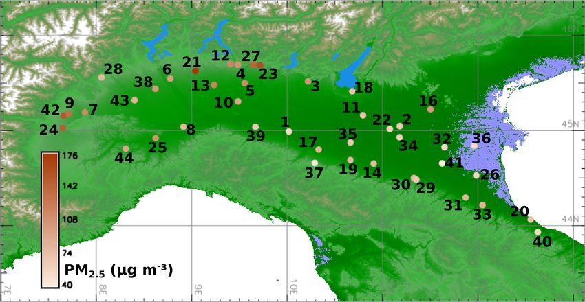
Figure 1. Location of PM2.5 monitoring stations included in the
All statistical data analyses were performed within the
analysis. The key for ID number is found in Table 1. Colour coding software environment R 3.2 (R Core Team, 2015).
refers to the result of the cluster analysis performed using a divi-
sive algorithm: sites within the same cluster have the same colour. 2.1 Trend estimate
Site 28 (Biella) resulted in an outlier and was not included in this
classification. Results of the cluster analysis with partition around The analysis for the presence of a trend involved a subset
medoids algorithm are in Fig. S3. More details are in Sects. 2.3 and of 24 PM2.5 series out of 44, i.e. the ones having a record
3.3. between 7 and 10 years long, and all 15 PM10–2.5 series,
with a length ranging between 7 and 9 years. The limit of
7 years for the sampling duration for a trend analysis results
undergo a daily, seasonal and annual comparison with nearby from the compromise between the spatial and temporal rep-
sites as well as with previous data. The authors have double- resentativeness of the valley by the analysed dataset. Simi-
checked the data by analysing annual, monthly, weekly and larly to the previous analysis for PM10 , slopes were estimated
daily patterns for all sites and by removing any occasional for monthly mean and annual quantiles of daily data, where
biased value (e.g. peaks from festival bonfires). A total of these statistics were computed if at least 75 % of the daily
15 out of these 44 sites included daily gravimetric equiva- data were available for the respective month or year.
lent measurements of PM10 . At these 15 sites the mass con- Monthly average concentrations were decomposed in
centration of coarse particles (PM10–2.5 ) was computed and trend, seasonal and remainder components by the seasonal
analysed equivalently to PM2.5 . trend decomposition procedure based on LOESS (STL)
The variability in atmospheric particle concentration was (Cleveland et al., 1990). For a good performance, STL re-
compared to provincial emission estimates of PM10 , PM2.5 , quires a clear seasonality in the analysed time series: this
CH4 , CO and other main particle precursors (SO2 , NOx , non- feature was shown by all PM2.5 series and by only two
methane volatile organic carbon (NMVOC) and NH3 ). Emis- PM10–2.5 series (see Sect. 3.1). All time series were log-
sions were provided by the National Institute for Environ- transformed prior to STL decomposition in order to achieve
mental Protection and Research (ISPRA) for the years 1990, normally distributed residuals and to control heteroscedas-
1995, 2000, 2005 and 2010 (inventory version 22_05_2015). ticity, and the analysis of monthly trend time series was per-
Provincial emissions are estimated by attribution of the na- formed on back-transformed logarithmic trend data. Gener-
tional emissions to each Italian province by a top-down pro- alized least squares (GLS) (Brockwell and Davis, 2002) and
cedure. Further details on the inventory used can be found model-based resampling (Davison and Hinkley, 1997) meth-
in the companion paper and references therein. Similarly to ods were used to estimate the presence of a significant slope
the companion study, only provinces with a significant part in trend components. Details on these methods can be found
of their land within the Po Valley were considered, assum- in Bigi and Ghermandi (2014). All resulting slopes and two
ing that most of the emissions occur in the valley part of the sample graphs are shown in Table 2 and in Fig. 2 respectively.
province, where most of the activities occur and the popu- Similarly to in the companion study, the trends of monthly
lation resides, instead of the mountainous parts. It is worth data were compared to non-parametric trends of annual quan-
noting that there are some large differences between the in- tiles: the slope of the 5th, 50th and 95th annual quantiles was
ventory version used in this study and the one used in the estimated by the Theil–Sen (hereafter TS) method; signifi-
companion paper, mostly related to emissions for SNAP sec- cance test for slope on annual data was performed by non-
tor 2 (i.e. commercial, institutional and residential combus- parametric resampling as in Yue and Pilon (2004). Result-
tion plants), where SNAP is the Standardized Nomenclature ing slopes for annual quantiles are shown in Table 3. Finally
for Air Pollutants. In this study we also included the emis- each month was tested for the presence of a trend: PM2.5 and
sion inventory for the Lombardy region: this is built with a PM10–2.5 daily concentration for each month was binned in
bottom-up procedure, based on emission source databases 10 µg m−3 increments, and the frequency of each bin in each
at a municipality level, and it is available for the years month over the sampling period was computed. The trend in
www.atmos-chem-phys.net/16/15777/2016/ Atmos. Chem. Phys., 16, 15777–15788, 201615780 A. Bigi and G. Ghermandi: Trends of PM2.5 and PM10–2.5 in the Po Valley
Table 2. Analysis of trend for monthly mean and for monthly frequency of PM2.5 and PM10–2.5 . Slope (± standard error) for monthly mean
is computed by generalized least squares (GLS) on deseasonalized monthly mean time series of daily PM2.5 or PM10–2.5 concentration.
Boldfaced values indicate slope significantly different from zero at a 95 % confidence level. Variation in monthly frequency distribution was
estimated by Theil–Sen method.
Station Slope Change Months with significant trend
µg m−3 yr−1 % yr−1
PM2.5
Besenzone −0.008 ± 0.121 0.0 % ± 0.5 % 5–6 (−), 12 (−)
Borgofranco −1.007 ± 0.139 −3.7 % ± 0.5 % 1–2 (−), 4 (−), 10 (−)
Brescia −1.323 ± 0.249 −4.3 % ± 0.8 % 1–2 (−), 3 (+), 5–6 (−), 12 (−)
Calusco d’Adda −1.428 ± 0.183 −5.4 % ± 0.7 % 1–2 (−), 4–5 (−), 7 (−), 9 (−), 11–12 (−)
Casirate d’Adda −1.035 ± 0.395 −3.2 % ± 1.2 % 1 (−), 11 (−)
Castano Primo −2.217 ± 0.177 −8.1 % ± 0.7 % 1–2 (−), 4 (−), 10 (−), 12 (−)
Chivasso −0.411 ± 0.174 −1.3 % ± 0.6 % 1–3 (−), 6 (±), 9–11 (−)
Cornale −0.953 ± 0.262 −4.5 % ± 1.3 % 1–2 (−), 4 (−), 9–10 (−)
Leinì −1.899 ± 0.969 −6.7 % ± 3.4 % 1–5 (−), 7 (−), 11–12 (−)
Lodi −1.605 ± 0.124 −6.4 % ± 0.5 % 2–12 (−)
Mantua −1.090 ± 0.269 −3.7 % ± 0.9 % 2 (−), 3 (±), 4–5 (−), 9–12 (−)
Merate −1.322 ± 0.427 −4.6 % ± 1.5 % 1 (−), 4–5 (−), 9–10 (−)
Milan −0.186 ± 0.154 −0.6 % ± 0.5 % 1–2 (−), 3–4 (+), 9 (−), 10 (±), 12 (−)
Modena −1.007 ± 0.402 −4.8 % ± 1.9 % 1 (−), 5–6 (−), 8–11 (−)
Mortara −1.439 ± 0.214 −5.5 % ± 0.8 % 1–2 (−), 4–5 (−), 8 (−), 10 (−)
Padua −1.271 ± 0.155 −3.9 % ± 0.5 % 1 (−), 3 (−), 11 (−)
Parma −0.648 ± 0.176 −3.2 % ± 0.9 % 1 (−), 3 (+), 5 (−), 12 (−)
Ponti sul Mincio −0.103 ± 0.212 −0.4 % ± 0.8 % 2 (−), 3 (+), 4 (−), 9 (+), 10 (−), 12 (−)
Reggio Emilia −0.819 ± 0.153 −3.8 % ± 0.7 % 1–2 (−), 3 (+), 5 (−), 12 (−)
Rimini −0.486 ± 0.245 −2.2 % ± 1.1 % 2 (−), 3 (+)
Saronno −0.844 ± 0.156 −3.0 % ± 0.5 % 1–2 (−), 5 (−), 12 (−)
Schivenoglia −0.496 ± 0.224 −1.9 % ± 0.8 % 1–2 (−), 4 (−), 8 (+), 10–11 (−)
Seriate −0.935 ± 0.075 −3.5 % ± 0.3 % 1 (−), 5 (−), 7 (−), 10 (−), 12 (−)
Turin Lingotto −1.717 ± 0.270 −5.2 % ± 0.8 % 1–2 (−), 4–5 (−), 7 (−), 9–11 (−)
PM10–2.5
Lodi −0.362 ± 0.248 −2.2 % ± 1.5 % 1–2 (−), 4 (±), 10 (−)
Merate −0.806 ± 0.280 −6.3 % ± 2.2 % 1–12 (−)
these frequencies for each month was estimated by the TS seasonal series (i.e. winter – January, February, March, and
method, and its significance was tested by a non-parametric summer – June, July, August) and focussed on PM anoma-
bootstrap, similarly as for the annual quantiles. For each site, lies, similarly to Bigi and Ghermandi (2014): the Kruskal–
months with a significant trend are listed in the rightmost col- Wallis test on weekly cycle of mean anomalies (WCY) and
umn of Table 2 and two sample graphs are in Fig. 3. Contrar- the Wilcoxon test on weekend effect magnitude (WEM).
ily to deseasonalized monthly means, these two latter trend Their significance was double-checked by repeating WCY
estimates were performed on all 24 PM2.5 + 15 PM10–2.5 and WEM tests on anomalies grouped into 6- and 8-day
sites. weeks (Barmet et al., 2009).
The TS method was used to estimate also trends in the The third test involved the analysis of the smoothed pe-
emission inventory data, along with non-parametric resam- riodogram for each time series of anomalies and verified
pling to asses the slope significance. the presence of a significant signal with a 7-day periodic-
ity above background noise. The periodogram estimates the
2.2 Weekly pattern spectral density of a continuous time series, showing the con-
tribution by all frequency components (eventually associated
In order to investigate the presence of a weekly cycle in to a specific process/source) to the variance of the series. The
daily PM2.5 and PM10–2.5 (i.e. a significantly different con- periodogram, in order to be estimated, needs a continuous
centration on a single weekday), three tests were used for series: in each time series, 1-day gaps were filled by lin-
all 44 + 15 series. Two tests involved both the complete and ear interpolation of neighbouring data, and the periodogram
Atmos. Chem. Phys., 16, 15777–15788, 2016 www.atmos-chem-phys.net/16/15777/2016/A. Bigi and G. Ghermandi: Trends of PM2.5 and PM10–2.5 in the Po Valley 15781
Table 3. Analysis of trend for annual quantiles of PM2.5 and PM10–2.5 . Slope for annual quantiles is computed by the Theil–Sen method:
boldface values indicate slope significantly different from zero at the 95 % confidence level.
5th annual quantile 50th annual quantile 95th annual quantile
Station Slope Change Slope Change Slope Change
µg m−3 yr−1 % yr−1 µg m−3 yr−1 % yr−1 µg m−3 yr−1 % yr−1
PM2.5
Besenzone 0.000 0.0 0.000 0.0 0.608 1.1
Borgofranco −0.667 −8.3 −1.000 −4.8 −1.087 −1.8
Brescia −0.250 −4.1 −0.367 −1.5 −2.272 −3.0
Calusco d’Adda −0.792 −13.1 −1.333 −7.0 −4.179 −6.1
Casirate d’Adda −0.225 −2.7 −0.225 −1.0 −3.917 −4.9
Castano Primo −0.286 −4.9 −0.857 −4.6 −3.421 −5.4
Chivasso 0.200 3.7 −0.817 −3.2 −1.531 −2.0
Cornale −0.500 −8.5 −1.000 −6.5 −4.383 −9.4
Leinì −0.100 −2.4 −2.333 −13.2 −10.800 −17.9
Lodi −0.929 −12.2 −2.000 −10.3 −1.875 −3.2
Mantua −0.412 −6.4 −2.000 −8.1 −4.225 −6.0
Merate −0.081 −1.0 −0.667 −3.0 −1.646 −2.3
Milan 0.000 0.0 0.200 0.9 −3.260 −4.3
Modena −0.333 −5.4 −1.200 −7.7 −4.000 −7.6
Mortara −0.930 −12.9 −1.000 −5.2 −2.988 −4.7
Padua −0.380 −4.4 −1.583 −6.6 −2.556 −3.0
Parma −0.500 −10.0 −0.667 −4.5 −1.000 −2.0
Ponti sul Mincio 0.071 1.3 0.000 0.0 −1.037 −1.7
Reggio Emilia −0.400 −6.7 −0.500 −3.0 −1.850 −3.7
Rimini −0.025 −0.5 0.000 0.0 −0.787 −1.4
Saronno −0.950 −23.8 −0.414 −2.1 −3.587 −4.7
Schivenoglia 0.000 0.0 0.500 2.3 −1.450 −2.5
Seriate −0.208 −3.7 −0.500 −2.5 −2.875 −4.1
Turin Lingotto −0.134 −2.2 −1.083 −4.8 −3.568 −4.1
PM10–2.5
Borgofranco −0.500 −60.0 0.000 0.0 1.060 5.4
Brescia −0.025 −5.4 −0.775 −8.2 −1.619 −6.7
Calusco d’Adda 0.000 0.0 0.000 0.0 0.000 0.0
Casirate d’Adda −0.250 −16.7 −0.375 −3.8 −1.900 −6.8
Lodi −0.100 −2.7 −0.200 −1.6 −0.180 −0.5
Mantua 0.000 0.0 −0.550 −8.7 −1.667 −9.2
Merate −0.500 −12.1 −0.917 −8.4 −2.417 −9.2
Milan −0.333 −23.3 −0.750 −6.4 −1.167 −4.3
Parma 0.738 23.4 0.000 0.0 0.217 0.9
Ponti sul Mincio −0.667 −29.9 −1.400 −14.4 −2.310 −9.6
Reggio Emilia 0.000 0.0 −0.333 −3.7 −1.367 −6.6
Rimini −0.500 −14.2 −0.750 −7.6 −1.538 −7.9
Saronno −0.250 −25.0 −0.536 −5.8 −1.434 −6.1
Schivenoglia −0.492 −55.2 −0.292 −4.4 1.673 8.9
Turin Lingotto 0.000 0.0 −0.600 −6.5 −1.000 −4.3
was computed from the resulting longest continuous record nificance of peaks in the periodogram was verified assum-
within the series. Following Mann and Lees (1996), pe- ing a χ 2 distribution for spectral estimates. Therefore a peak
riodogram smoothing was achieved by the multiple-taper in the smoothed periodogram at the frequency 1/7 day−1 is
method (MTM), and background noise was estimated as an significant when exceeding the 95 % confidence bands for
AR(1) red noise process, whose lag-1 autocorrelation coef- red noise at that same frequency (suggesting the presence of
ficient proceeds from a robust estimate. The statistical sig- a periodic emission source inducing a similar periodicity in
www.atmos-chem-phys.net/16/15777/2016/ Atmos. Chem. Phys., 16, 15777–15788, 201615782 A. Bigi and G. Ghermandi: Trends of PM2.5 and PM10–2.5 in the Po Valley
80
●
●
●
●
●
●
●●
● ●
60
● ●
● ●
●
PM2.5 (µg m−3)
●
●● ●
●
●
●● ●
● ● ● ● ●●
●
● ●
●●
40
● ●
● ● ● ● ●
●● ●
●
● ●
● ● ●
● ● ● ●● ●
● ●
● ● ●
●● ● ●
● ●● ●
● ●
20
● ●● ●
● ●
● ● ●
● ● ● ● ● ● ● ●
● ● ● ● ● ●● ● ●
● ● ●● ● ●●
● ● ● ● ●
● ● ●
● ●
●
Padua
0
● Monthly mean concentration STL trend component
STL Trend + seasonal component GLS fitted model
80
●
●
●
● ●
PM2.5 (µg m−3)
●
60
●
● ● ●
● ●
● ●
● ●●
●
● ●
● ● ●
● ●
40
●
●
● ● ●
● ● ● ●
● ●
● ● ●
● ● ● ● ●
● ● ● ●●
● ● ●
● ● ● ●
20
● ●
● ●
● ● ● ●
● ●
● ● ●● ●●
● ●●● ●● ● ●● ● ● ●
● ● ● ●●
● ● ● ●
● ●●● ●
● ● ● ●● ●
●
● ●
Saronno
0
2006 2008 2010 2012 2014
Figure 2. STL decomposition for monthly mean PM2.5 along with
generalized least squares (GLS) fitted slope for two selected sites.
atmospheric pollutant concentration). The astrochron pack-
age in R (Meyers, 2012) was used to follow the approach by
Mann and Lees (1996). Results for the weekly cycle analysis
are presented in Table S1 in the Supplement and anomalies
for PM2.5 and PM10–2.5 are shown in Fig. S1 and S2. Figure 3. Significant changes in monthly frequency distribution of
PM2.5 at Milan (a) and Mortara (b).
2.3 Cluster analysis
Cluster analysis was performed only on PM2.5 daily data and and resampling techniques, to minimize the influence of un-
included all 44 sites. Several distance metrics and clustering common weather conditions on the estimated trends. Finally,
algorithms were tested. Best results were chosen depending the influence of a possible long-term trend in meteorological
on the cluster silhouette and the overall performance index, variables as temperature or precipitation was estimated to be
which led to two slightly different outcomes: one generated negligible over the comparatively short length of these PM
by divisive hierarchical clustering algorithm and one by par- series.
tition around medoids (Kaufman and Rousseeuw, 1990). In A main assumption in the discussion of trends and patterns
the former an outlying site (Biella, ID 28) was removed from is that, notwithstanding the occasional influence of long-
the dataset to prevent classification fouling (Kaufman and range transport on PM in the Po Valley (e.g. Masiol et al.,
Rousseeuw, 1990). For both algorithms the dissimilarity ma- 2015), we considered local emission sources to have the
trix was based on a Pearson’s correlation coefficient metric largest influence on particulates in the Po Valley: throughout
(see Bigi and Ghermandi, 2014), highlighting linear correla- the analysis we assumed trends in continental emissions to
tion structures among sites. Spatial representation of the two have a minor effect on the estimated PM trends. A reasonable
resulting set of clusters is found in Figs. 1 and S3. assumption, particularly in winter when valley emissions are
confined for long periods within the (often shallow) mixing
layer.
3 Results and discussion
3.1 Results from trend analysis
General comments on the pre-processing procedures and
trends used in the companion paper apply to this study: we All estimated trends are assumed linear. This was mostly
exploited the STL performance on extracting the trend com- true for all trend components extracted by STL on monthly
ponent from the monthly data, featured by wide seasonality, PM2.5 , while only in Lodi and Merate did monthly-mean
and we took advantage of the robustness of both quantiles PM10–2.5 show a sufficiently wide seasonal pattern to allow
Atmos. Chem. Phys., 16, 15777–15788, 2016 www.atmos-chem-phys.net/16/15777/2016/A. Bigi and G. Ghermandi: Trends of PM2.5 and PM10–2.5 in the Po Valley 15783
a reliable extraction of a seasonal and a trend component by sources over time (e.g. construction works) and leading non-
STL, with the latter being linear. Not surprisingly, these two parametric bootstrap to negate slope significance, notwith-
sites are urban traffic stations and recorded the largest PM standing that a clear slope is present, as in the case of Rimini
coarse concentration among all investigated sites (their over- 95th quantile (see Fig. S4 for PM10–2.5 annual trends).
all mean is 16.2 and 12.7 µg m−3 respectively). Trends in PM10–2.5 found by Barmpadimos et al. (2012) at
The trend component for monthly PM2.5 showed a signifi- five EMEP sites are largely smaller than the ones observed in
cant decline at most sites, ranging from 0.5 to 2 µg m−3 yr−1 this study, supporting the hypothesis of the influence by pri-
(Table 2). PM2.5 annual quantiles exhibited a decline at sev- mary sources on Po Valley sites. Very few other studies in-
eral sites (Table 3), indicating a decrease for large, median vestigated trends for PM10–2.5 in Europe. Amato et al. (2014)
and low concentration levels. Significant decrease rate for an- found a trend of −1.5/−2 µg m−3 yr−1 in road dust in south-
nual median was highly similar to the GLS trend of monthly ern Spain (meteorologically very different from the Po Val-
mean at the corresponding site (e.g. Borgofranco, Cornale, ley) and ascribed it to the decrease in construction works due
Parma); missing data or outliers in the annual series led the to the severe financial crisis: from the data available for this
significance test for slope to fail at several sites, although the study a similar explanation does not apply to the PM10–2.5
data showed a clear trend. trends observed in the Po Valley.
In order to detect months with a concentration change over
the analysed period, TS trends in frequency of monthly bins
3.2 Results for weekly pattern
were computed (see Fig. 3 for the results at two sites). In
the rightmost column of Table 2, a − sign next to a specific
month indicates a decrease in frequency of higher concen- Three different tests were used to assess whether a significant
tration bins towards lower bins, a + sign a shift from lower weekly pattern was present. Results presented in Table S1
to higher concentration bins, and a ± sign a shift in lower show how, to some extent, the tests confirm each other, with
and higher concentration bins towards median concentra- WCY and WEM outperforming MTM. Almost all PM2.5
tions. The analysis of binned concentration levels indicates sites exhibit a significant weekly pattern in summer, how-
that at most sites higher concentrations decreased, mostly ever almost none in winter. A weekly periodicity is observed
during winter months with January and February being the in PM10–2.5 at almost all sites both in winter and in sum-
most frequent (see the rightmost column in Table 2). Occa- mer, as expected given the most common sources of coarse
sional decrease of higher concentrations was observed also particles. For both PM fractions, significance in weekly pe-
in summer months, while an increase in lower concentrations riodicity was supported by the negative result of tests on 6-
was found in spring at few sites. These results are partly con- and 8-day weeks. This is consistent with the findings in Bigi
sistent with slopes in fifth annual quantile, representative of and Ghermandi (2014), where a significant weekly pattern
spring–summer trends. As a matter of comparison, estimates in PM10 was found in winter only at older sites (i.e. acti-
of trends for PM2.5 annual mean at several EMEP (Euro- vated before 2002): this was ascribed to a larger contribution
pean Monitoring and Evaluation Programme) sites, i.e. rural by the coarse fraction to PM10 in late 1990s early 2000s, as
background, over 2002–2010 by Cusack et al. (2012) were confirmed by the decrease in PM10–2.5 reported here. Similar
between ∼ −3.8/ − 5.4 % yr−1 , similar to significant trends results are in the study by Barmpadimos et al. (2011b), where
occurring in the Po Valley for annual median at background for seven different sites in Switzerland a significant weekly
sites (e.g. Borgofranco, Chivasso or Parma). cycle was found, both in PM2.5 and PM10–2.5 , including the
The trend component of monthly PM10–2.5 at Lodi and rural background site of Payerne.
Merate showed a drop of 2 and 6 % yr−1 respectively; in Lodi One of the most recent source apportionment studies of
only winter months significantly contributed to this drop, PM2.5 in the Po Valley, by Perrone et al. (2012), based on
whereas in Merate this drop occurred throughout the year. samples over 2006–2009 in urban background Milan, esti-
At Merate also annual quantiles exhibit a significant trend, mates the contribution of SIA and biomass burning (BB) to
while at Lodi the nonlinearity and a missing data lead to be larger in PM2.5 than in PM10 , and higher in winter than in
a non-significant slope. Both these are traffic sites and are summer (up to 53 % in winter PM2.5 ). These results are con-
directly affected by primary sources of coarse particles, i.e. sistent with the scientific literature (Finlayson-Pitts and Pitts,
motor exhausts and road, tire and break wear (either directly 2000) and are confirmed by the findings of other recent PM
emitted or resuspended) (e.g. see Perrone et al., 2012, for source apportionment studies in the Po Valley (e.g. Larsen
a PM source apportionment in Milan). This outcome sug- et al., 2012), i.e. supporting the hypothesis of a buffering role
gests that the previously observed decrease in PM10 (Bigi by SIA+BB over sources having a weekly periodicity (e.g.
and Ghermandi, 2014) is partly due to a drop in exhaust traffic, industry, resuspension), whose relative contribution is
traffic emission following the renewal of the vehicular fleet, estimated to be lowest in winter PM2.5 and highest in sum-
at least at traffic sites. Indeed the trend in PM10–2.5 annual mer PM10–2.5 . Interesting enough, for both PM fractions the
quantiles shows some site dependency along with several significance in weekly periodicity is not dependent on station
cases of nonlinearity, suggesting occasional changes in active classification according to the air-quality network: this also
www.atmos-chem-phys.net/16/15777/2016/ Atmos. Chem. Phys., 16, 15777–15788, 201615784 A. Bigi and G. Ghermandi: Trends of PM2.5 and PM10–2.5 in the Po Valley
supports the assumption on the minor influence of continen- Over the period 2005–2014 the total number of passen-
tal emission trends. ger cars and light-duty vehicles (LDVs) in the Po Valley was
almost constant (∼ −0.02 %), with the mean age of gaso-
3.3 Results from cluster analysis line and diesel passenger cars increasing to ∼ 3 years. Note
that diesel cars are on average 6 years younger than gasoline
Similarly to Po Valley PM10 , also PM2.5 exhibited a strong ones, consistent with the dieselization of the fleet observed
seasonality, a significant trend and changes in frequency dis- in most of Europe (EEA, 2015a). Over the same period, fuel
tribution across the valley (note that the PM2.5 / PM10 ratio sales showed a significant linear trend for unleaded gasoline
in the Po Valley is approaching 1 over the years, particularly (−6.2 % yr−1 ), a mild decline for diesel (−0.8 % yr−1 ) and
at urban sites and in winter). Similarly to the companion an increase for LPG (6.9 % yr−1 ). This drop in fuel sales is
paper, cluster analysis allowed us to highlight the presence ascribed to both the renewal of the fleet, i.e. the increased
of groups having large internal correlation and showed how number of vehicles with a more efficient engine, and to a re-
the spatial distribution of most similar sites derives mainly cent level-off (decrease) of the mean distance travelled by car
from their geographical position instead of their classifica- according to EEA (2015b) (ACI, 2012).
tion within the air-quality network. Nonetheless, some dif- The observed trends in atmospheric PM2.5 occurred at sev-
ferences between the outcome of cluster analysis applied eral sites, including the rural background stations of Cornale
to PM10 and PM2.5 exist: three or two clusters resulted for and Schivenoglia; the drop occurred more often in winter,
PM2.5 depending on the algorithm used (Figs. 1 and S3), i.e. when no site exhibits a weekly cycle (i.e. a significant im-
fewer than for PM10 (as expected spatial variability for finer pact of primary anthropogenic emissions) and ranged from
particles is smaller). The influence of the metropolitan ar- ∼ −1 % to ∼ −8 % yr−1 . Decrease was largest (in absolute
eas, evident for PM10 , is not shown by PM2.5 . Eastern and and relative terms) at traffic urban sites and became lower
western part of the valley were split into fewer groups when from urban towards rural sites (see Fig. 4), although the small
analysed for PM2.5 , compared to PM10 . That is, a difference dataset did not allow us to robustly test for a significant dif-
in PM2.5 between eastern and western Po Valley exists. How- ference in trends among station types. From an overview of
ever, within each side of the valley PM2.5 levels are more cor- some recent source apportionment and chemical composi-
related than PM10 levels. Resulting clusters have to be under- tion studies of PM2.5 in the Po Valley (Carbone et al., 2010;
stood as flexible, with sites on the “geographical boundary” Khan et al., 2016; Larsen et al., 2012; Masiol et al., 2015;
between two groups having a weaker membership. Matta et al., 2003; Perrino et al., 2013; Perrone et al., 2012;
Pietrogrande et al., 2016) primary traffic emissions (includ-
3.4 Results from emission trend analysis and discussion
ing exhaust and non-exhaust) are highest at traffic sites in
PM2.5 and PM10–2.5 investigated in this study refer to the pe- absolute and relative terms, decreasing towards rural back-
riod 2005–2014, while valley-wide emission data are avail- ground sites, suggesting that the decrease in PM2.5 emissions
able every 5 years over the period 1990–2010, preventing any by traffic had a significant role in the observed trends in at-
tentative comparison between the trends of the two datasets, mospheric composition.
only a qualitative assessment. Moreover, as shown by Fi- This possibility is supported by chemical transport model
nardi et al. (2014) with an Eulerian chemical transport model, simulations of de Meij et al. (2009). The latter authors es-
change in emissions in the Po Valley leads to highly non- timated that a single drop in total PM2.5 emissions of only
linear change in atmospheric pollutants levels (e.g. O3 , OH. ∼ 200 Mg for SNAP 7 across Lombardy would lead to a
and NO− variation of −2.3 µg m−3 in primary PM2.5 in the Milan
3 ) and in PM in general: this would make trends in
emissions and PM even harder to compare. metropolitan area. According to the Lombardy inventory, pri-
SNAP sector 1 (best represented by power plants) showed mary PM2.5 emissions by SNAP 7 actually drop ∼ 2000 Mg
a large decrease in SO2 , NOx and PM emissions, and its con- over 2005–2012, while the ISPRA provincial inventory esti-
tribution to Po Valley emissions is minor, particularly since mated a drop of ∼ 2500 Mg over 2005–2010. Over the same
2005 (see Fig. S5). A significant reduction occurred in NOx , period, the observed mean absolute drop in monthly PM2.5
NMVOC and PM emissions by road transport SNAP 7, one for Lombardy resulted in ∼ 10 µg m−3 . Given the increase in
of largest sources in the valley. The modest contribution of PM emissions by heating in winter counterbalancing the drop
emissions by industrial combustion (SNAP 3) decreased fur- in SNAP 7 (and in SNAP 3), the observed downward trend in
ther for SO2 , NOx and PM, both by technological improve- atmospheric levels is potentially consistent with the outcome
ments and recent national economy slowdown. On the con- by de Meij et al. (2009) and partly generated by a drop in pri-
trary, heating (SNAP 2) exhibits an increase in emission of mary traffic emissions (potentially exhaust and non-exhaust).
several species (e.g. NOx , NMVOC and PM2.5 ), most likely A drop in atmospheric SIA is also expected due to the large
due to an increase in the use of biomass, notwithstanding that decrease in NOx emissions and the (relatively modest) drop
this is a seasonal source. These trends were observed in both in NH3 (∼ 17 000 Mg according to ISPRA provincial inven-
analysed inventories. tory); this would be consistent with the decrease of nitrate,
ammonium and sulfate ion concentration in fog at the rural
Atmos. Chem. Phys., 16, 15777–15788, 2016 www.atmos-chem-phys.net/16/15777/2016/A. Bigi and G. Ghermandi: Trends of PM2.5 and PM10–2.5 in the Po Valley 15785
0.0
started around the year 2000. Rimini experienced a decrease
0.0
in PM10 of ∼ 1 µg m−3 yr−1 , while PM2.5 and PM10–2.5 de-
creased by ∼ 0.5 µg m−3 yr−1 each, suggesting that both
primary and SIA significantly contributed to the change in
−0.5
−1.6
PM10 atmospheric concentration. Similar changes occurred
in Parma, where the trends were significant for both PM10
and PM2.5 ; at the latter site it is worth noting that the increase
Slope ( µg m−3 yr−1)
−1.0
−3.2
Change (% yr−1)
observed in the fifth quantile of PM10 is present (although
not significant) for this same quantile of PM10–2.5 . Finally,
similar results apply to Reggio Emilia, i.e. to the other site
−1.5
−4.8
included both in the present study and in the companion pa-
per.
−2.0
−6.4
3.5 Analysis of valley-wide episodes
●
Two consecutive and worth noting PM2.5 pollution episodes
−2.5
−8.0
●
occurred in 2012: the first from 16 to 23 January 2012 and
the second from 15 to 19 February 2012. These episodes are
RB SuB UB UI UT
briefly presented as representative, although extreme, exam-
Figure 4. Boxplot of absolute and percentage significant slope of ples of valley-wide PM events.
deseasonalized monthly mean PM2.5 by station type. The episode in January was generated by a persistent in-
version layer confining surface emissions; 12:00 UTC ra-
diosoundings at Milan Linate Airport showed thermal inver-
background station San Pietro C. over the period 1990–2011 sions up to 10 ◦ C, at a height between ∼ 200 and ∼ 500 m
(Giulianelli et al., 2014). In agreement, simulation results by throughout the event. PM2.5 concentration was largest in the
de Meij et al. (2009) showed a significant drop in SIA only N–NW sector of the valley (i.e. at the foothill of the Alps) and
with a concurrent decrease in NOx and NH3 emissions. decreased towards S–SE. The peak in daily PM2.5 during this
Available data do not allow the assessment of whether also event represented the maximum record ever for several sites
a variation in secondary organic aerosol (SOA) occurred: (e.g. Bergamo, Turin Caduti) and is equal to or above the re-
NMVOC and NOx , whose emissions drop over the inves- spective 94th quantile for all other sites (see Fig. S6). The
tigated period, have a competing effect on SOA formation severity of the event was locally mitigated thanks to aerosol
(Andreani-Aksoyoglu et al., 2004), and meanwhile biomass deposition by the several fog precipitation events which oc-
burning emissions increased. The latter is a large source of curred across the valley, triggered by the high relative humid-
both primary and secondary OC (e.g. Piazzalunga et al., ity (similarly to the process shown by Gilardoni et al., 2014,
2011; Gilardoni et al., 2011; Ozgen et al., 2014), contributing during the fog scavenging events of winter 2011).
to the large levels of SOA found in winter PM in the Po Val- The second episode occurred during the European cold
ley (e.g. Khan et al., 2016; Larsen et al., 2012; Perrino et al., wave in February 2012, when in most of the valley the cold-
2013; Pietrogrande et al., 2016). Indeed Putaud et al. (2014) est temperature over the last ∼ 60 years was observed. In the
found a significant trend in PM2.5 mass and optical properties first days of February large snowfalls occurred over the val-
at the Ispra EMEP site over 2004–2010. This trend was ex- ley (leading to a 100-year peak in snow height across the
plained by an increment in brown carbon, i.e. in OC content, E sector), followed by several days of clear-sky conditions,
most likely originating from an increase in biomass burning i.e. when the episode occurred. This event featured extremely
emissions. The slower decrease in PM at rural sites compared cold temperatures and thermal inversions at night, confining
to urban ones might be eventually due also to the wider use of the intense emissions by heating, and warm–dry conditions
biomass for heating in rural areas, consistent with the spatial at daytime, with a diurnal temperature variation up to 15 ◦ C
results of the simulations by de Meij et al. (2009). and with either a minor inversion or an isothermal profile at
Finally, the results from the present study hint to a ratio- noon (by radiosounding profile at Milan). The episode was
nale to explain the decreasing trends previously found for ended by precipitation which occurred on 20 February. This
PM10 in the Po Valley (Bigi and Ghermandi, 2014) over second PM2.5 episode was more severe than the former, with
1998–2012: these seem to originate from a drop in the frac- PM2.5 concentration peaking at 186 µg m−3 (see Fig. S7).
tion of both primary particles and SIA, with their respec- For both events we computed 36 h long backtrajectories
tive role in the observed trends being site-dependent. This by HYSPLIT (Draxler and Rolph, 2013) using 0.5◦ GDAS
rationale is supported by the decrease in PM10–2.5 at Lodi meteorological data, and the results refute the possibility of
and Merate (traffic sites) and at several UB sites, partly be- a transboundary pollution episode.
cause of the still ongoing technology renewal, a process that
www.atmos-chem-phys.net/16/15777/2016/ Atmos. Chem. Phys., 16, 15777–15788, 201615786 A. Bigi and G. Ghermandi: Trends of PM2.5 and PM10–2.5 in the Po Valley
4 Conclusions The Supplement related to this article is available online
at doi:10.5194/acp-16-15777-2016-supplement.
Analysis of the trend, of the weekly periodicity, and of the
similarity in PM2.5 and PM10–2.5 concentration time series
in the Po Valley was performed. The trend was estimated
by generalized least squares (GLS) on monthly deseasonal- Acknowledgements. Authors acknowledge ARPA Emilia-
ized time series, by the TS method on annual quantiles and Romagna, ARPA Lombardia, ARPA Piemonte and ARPA Veneto
by the TS method on frequency of daily binned concentra- for providing the concentration data of atmospheric pollutants.
tion for each month. The slopes estimated by TS and GLS
on the same time series show good agreement. A significant Edited by: Y. Balkanski
and widespread decrease in monthly PM2.5 and PM10–2.5 oc- Reviewed by: three anonymous referees
curred at the investigated monitoring sites, most often dur-
ing colder months for the finest particle fraction, with slope
getting steeper from rural background towards urban traf- References
fic sites. Fewer cases of significant slopes occurred for an-
nual quantiles due to non-linearities, missing data and lim- ACI: Where is the car gone? XX report ACI-CENSIS (in Italian),
ited length of annual series. A significant weekly cycle (i.e. Tech. Rep. 20, Italian Automobile Club, Rome, Italy, http:
//www.aci.it/fileadmin/documenti/studi_e_ricerche/monografie_
possibly forced by anthropogenic emissions) was found for
ricerche/RAPPORTI_ACI_CENSIS/ACI-CENSIS_2012.pdf
several PM2.5 series. This periodicity occurred more often in
(last access: 16 December 2016), 2012.
summer, probably because of the lower contribution to PM Amato, F., Alastuey, A., de la Rosa, J., Gonzalez Castanedo, Y.,
by SIA and by biomass burning emission compounds during Sánchez de la Campa, A. M., Pandolfi, M., Lozano, A., Con-
warmer months, along with an increase of the primary parti- treras González, J., and Querol, X.: Trends of road dust emis-
cle fraction. For all PM10–2.5 series a significant weekly cy- sions contributions on ambient air particulate levels at rural, ur-
cle was found throughout the year. Notwithstanding that the ban and industrial sites in southern Spain, Atmos. Chem. Phys.,
investigated sites show similar trends and patterns, a hierar- 14, 3533–3544, doi:10.5194/acp-14-3533-2014, 2014.
chical cluster analysis of daily PM2.5 concentration showed Andreani-Aksoyoglu, S., Prévôt, A. S. H., Baltensperger, U., Keller,
some differences between western, eastern and southern ar- J., and Dommen, J.: Modeling of formation and distribution of
eas of the valley. secondary aerosols in the Milan area (Italy), J. Geophys. Res.,
109, D05306, doi:10.1029/2003JD004231, 2004.
Finally, the trends in atmospheric PM2.5 and PM10–2.5 con-
Anttila, P. and Tuovinen, J.: Trends of primary and secondary pol-
centration, in emissions, in the vehicular fleet composition,
lutant concentrations in Finland in 1994–2007, Atmos. Environ.,
and in fuel sales were compared: the results suggest that the 44, 30–41, doi:10.1016/j.atmosenv.2009.09.041, 2010.
observed drop in PM2.5 was generated by the renewal in ve- Avery, C. L., Mills, K. T., Williams, R., McGraw, K. A.,
hicular fleet over the Po Valley, i.e. the introduction of ve- Poole, C., Smith, R. L., and Whitsel, E. A.: Estimating er-
hicles having more efficient engines and improved emission ror in using ambient PM2.5 concentrations as proxies for
control systems, leading to a drop in the fraction of primary personal exposures: a review, Epidemiology, 21, 215–223,
particles and of SIA (triggered by the reduced NOx emis- doi:10.1097/EDE.0b013e3181cb41f7, 2010.
sions). Regarding PM10–2.5 , results suggest that a significant Barmet, P., Kuster, T., Muhlbauer, A., and Lohmann, U.: Weekly
decrease in primary coarse particulate emissions occurred cycle in particulate matter versus weekly cycle in precip-
until recently, again due to a technology renewal in the ve- itation over Switzerland, J. Geophys. Res., 114, D05206,
doi:10.1029/2008JD011192, 2009.
hicular fleet: most likely the latter is partly responsible for
Barmpadimos, I., Hueglin, C., Keller, J., Henne, S., and Prévôt, A.
the drop in atmospheric PM10 previously observed in the Po
S. H.: Influence of meteorology on PM10 trends and variability in
Valley in the companion paper. Switzerland from 1991 to 2008, Atmos. Chem. Phys., 11, 1813–
Study outlooks include the assessment of the role of SOA 1835, doi:10.5194/acp-11-1813-2011, 2011a.
and of emissions in neighbouring regions on the observed Barmpadimos, I., Nufer, M., Oderbolz, D., Keller, J., Aksoyoglu, S.,
trends. Hueglin, C., Baltensperger, U., and Prévôt, A.: The weekly cycle
of ambient concentrations and traffic emissions of coarse (PM10 –
PM2.5 ) atmospheric particles, Atmos. Environ., 45, 4580–4590,
5 Data availability doi:10.1016/j.atmosenv.2011.05.068, 2011b.
Barmpadimos, I., Keller, J., Oderbolz, D., Hueglin, C., and Prévôt,
The data used in this study are available at the Air A. S. H.: One decade of parallel fine (PM2.5 ) and coarse
Quality e-Reporting (AQ e-Reporting). Permalink to the (PM10 –PM2.5 ) particulate matter measurements in Europe:
current version is http://www.eea.europa.eu/ds_resolveuid/ trends and variability, Atmos. Chem. Phys., 12, 3189–3203,
c0483fb2753342cabda8e7b4f4fea3f7 (EEA, 2016). doi:10.5194/acp-12-3189-2012, 2012.
Bigi, A. and Ghermandi, G.: Long-term trend and variability of at-
mospheric PM10 concentration in the Po Valley, Atmos. Chem.
Phys., 14, 4895–4907, doi:10.5194/acp-14-4895-2014, 2014.
Atmos. Chem. Phys., 16, 15777–15788, 2016 www.atmos-chem-phys.net/16/15777/2016/A. Bigi and G. Ghermandi: Trends of PM2.5 and PM10–2.5 in the Po Valley 15787 Bigi, A., Ghermandi, G., and Harrison, R. M.: Analysis of the air Finardi, S., Silibello, C., D’Allura, A., and Radice, P.: Anal- pollution climate at a background site in the Po valley, J. Environ. ysis of pollutants exchange between the Po Valley and the Monitor., 14, 552–563, 2012. surrounding European region, Urban Clim., 10, 682–702, Bigi, A., Bianchi, F., De Gennaro, G., Di Gilio, A., Fermo, P., Gher- doi:10.1016/j.uclim.2014.02.002, 2014. mandi, G., Prévôt, A. S. H., Urbani, M., Valli, G., Vecchi, R., and Finlayson-Pitts, B. J. and Pitts, J. N.: Chemistry of the Upper and Piazzalunga, A.: Hourly composition of gas and particle phase Lower Atmosphere, Academic Press, San Diego, USA, 2000. pollutants at a central urban background site in Milan, Italy, Franklin, M., Zeka, A., and Schwartz, J.: Association between Atmos. Res., 186, 83–94, doi:10.1016/j.atmosres.2016.10.025, PM2.5 and all-cause and specific-cause mortality in 27 US com- 2017. munities, J. Expo. Sci. Env. Epid., 17, 279–287, 2006. Boldo, E., Medina, S., Le Tertre, A., Hurley, F., Mücke, H.-G., Gilardoni, S., Vignati, E., Cavalli, F., Putaud, J. P., Larsen, B. Ballester, F., and Aguilera, I.: Apheis: Health Impact Assess- R., Karl, M., Stenström, K., Genberg, J., Henne, S., and Den- ment of Long-term Exposure to PM2.5 in 23 European Cities, tener, F.: Better constraints on sources of carbonaceous aerosols Eur. J. Epidemiol., 21, 449–458, doi:10.1007/s10654-006-9014- using a combined 14 C – macro tracer analysis in a European 0, 2006. rural background site, Atmos. Chem. Phys., 11, 5685–5700, Brockwell, P. J. and Davis, R. A.: Introduction to Time Series and doi:10.5194/acp-11-5685-2011, 2011. Forecasting, 2nd edn., Springer-Verlag, New York, USA, 2002. Gilardoni, S., Massoli, P., Giulianelli, L., Rinaldi, M., Paglione, M., Carbone, C., Decesari, S., Mircea, M., Giulianelli, L., Finessi, Pollini, F., Lanconelli, C., Poluzzi, V., Carbone, S., Hillamo, R., E., Rinaldi, M., Fuzzi, S., Marinoni, A., Duchi, R., Perrino, Russell, L. M., Facchini, M. C., and Fuzzi, S.: Fog scavenging C., Sargolini, T., Vardé, M., Sprovieri, F., Gobbi, G., An- of organic and inorganic aerosol in the Po Valley, Atmos. Chem. gelini, F., and Facchini, M.: Size-resolved aerosol chemical Phys., 14, 6967–6981, doi:10.5194/acp-14-6967-2014, 2014. composition over the Italian Peninsula during typical sum- Giulianelli, L., Gilardoni, S., Tarozzi, L., Rinaldi, M., Dece- mer and winter conditions, Atmos. Environ., 44, 5269–5278, sari, S., Carbone, C., Facchini, M., and Fuzzi, S.: Fog doi:10.1016/j.atmosenv.2010.08.008, 2010. occurrence and chemical composition in the Po valley Cleveland, R. B., Cleveland, W. S., McRae, J., and Terpenning, I.: over the last twenty years, Atmos. Environ., 98, 394–401, STL: a seasonal-trend decomposition procedure based on Loess, doi:10.1016/j.atmosenv.2014.08.080, 2014. J. Off. Stat., 6, 3–33, 1990. Hicks, B., Artz, R., Meyers, T., and Hosker Jr., R.: Trends in eastern Cusack, M., Alastuey, A., Pérez, N., Pey, J., and Querol, X.: Trends U.S. sulfur air quality from the Atmospheric Integrated Research of particulate matter (PM2.5 ) and chemical composition at a re- Monitoring Network, J. Geophys. Res., 107, ACH 6–1–ACH 6– gional background site in the Western Mediterranean over the last 12, 2002. nine years (2002–2010), Atmos. Chem. Phys., 12, 8341–8357, Jonson, J. E., Simpson, D., Fagerli, H., and Solberg, S.: Can we ex- doi:10.5194/acp-12-8341-2012, 2012. plain the trends in European ozone levels?, Atmos. Chem. Phys., Davison, A. and Hinkley, D.: Bootstrap Methods and Their Appli- 6, 51–66, doi:10.5194/acp-6-51-2006, 2006. cation, Cambridge University Press, Cambridge, UK, 1997. Kaufman, L. and Rousseeuw, P. J.: Finding Groups in Data: an In- de Meij, A., Thunis, P., Bessagnet, B., and Cuvelier, C.: The sensi- troduction to Cluster Analysis, Wiley, New York, USA, 1990. tivity of the CHIMERE model to emissions reduction scenarios Khan, M. B., Masiol, M., Formenton, G., Gilio, A. D., on air quality in Northern Italy, Atmos. Environ., 43, 1897–1907, de Gennaro, G., Agostinelli, C., and Pavoni, B.: Carbona- doi:10.1016/j.atmosenv.2008.12.036, 2009. ceous PM2.5 and secondary organic aerosol across the Denby, B., Sundvor, I., Cassiani, M., de Smet, P., de Leeuw, Veneto region (NE Italy), Sci. Total Environ., 542, 172–181, F., and Horálek, J.: Spatial mapping of Ozone and SO2 doi:10.1016/j.scitotenv.2015.10.103, 2016. trends in Europe, Sci. Total Environ., 408, 4795–4806, Klimont, Z., Smith, S., and Cofala, J.: The last decade of global an- doi:10.1016/j.scitotenv.2010.06.021, 2010. thropogenic sulfur dioxide: 2000–2011 emissions, Environ. Res. Draxler, R. and Rolph, G.: HYSPLIT (HYbrid Single-Particle Lett., 8, 014003, doi:10.1088/1748-9326/8/1/014003, 2013. Lagrangian Integrated Trajectory), Model access via NOAA Larsen, B., Gilardoni, S., Stenström, K., Niedzialek, J., Jimenez, ARL READY Website, available at: http://www.arl.noaa.gov/ J., and Belis, C.: Sources for PM air pollution in the Po Plain, HYSPLIT.php (last access: 16 December 2016), 2013. Italy: II. Probabilistic uncertainty characterization and sensitivity EEA: Impact of selected policy measures on Europe’s air quality, analysis of secondary and primary sources, Atmos. Environ., 50, Tech. Rep. 8, EEA, doi:10.2800/42618, 2010. 203–213, doi:10.1016/j.atmosenv.2011.12.038, 2012. EEA: Dieselisation in the EEA, available at: http://www.eea.europa. Loomis, D., Grosse, Y., Lauby-Secretan, B., Ghissassi, F. E., eu/ds_resolveuid/9e1b1bc1198552e8e5eeae494ca938aa (last ac- Bouvard, V., Benbrahim-Tallaa, L., Guha, N., Baan, R., Mat- cess: 16 December 2016), 2015a. tock, H., and Straif, K.: The carcinogenicity of outdoor air EEA: Developments in fuel efficiency of an average car along- pollution, Lancet Oncol., 13, 1262–1263, doi:10.1016/S1470- side trends in private car ownership and greenhouse gas (GHG) 2045(13)70487-X, 2013. emissions, available at: http://www.eea.europa.eu/ds_resolveuid/ Mann, M. E. and Lees, J. M.: Robust estimation of background 358812e51f354427b9a161fd9c1d30d0 (last access: 16 Decem- noise and signal detection in climatic time series, Climate ber 2016), 2015b. Change, 33, 409–445, doi:10.1007/BF00142586, 1996. EEA: Air Quality e-Reporting (AQ e-Reporting), avail- Masiol, M., Benetello, F., Harrison, R. M., Formenton, G., Gas- able at: http://www.eea.europa.eu/ds_resolveuid/ pari, F. D., and Pavoni, B.: Spatial, seasonal trends and trans- c0483fb2753342cabda8e7b4f4fea3f7, last access: 19 December boundary transport of PM2.5 inorganic ions in the Veneto 2016. www.atmos-chem-phys.net/16/15777/2016/ Atmos. Chem. Phys., 16, 15777–15788, 2016
You can also read