TOWARDS UNKNOWN-AWARE DEEP Q-LEARNING
←
→
Page content transcription
If your browser does not render page correctly, please read the page content below
Under review as a conference paper at ICLR 2022

T OWARDS U NKNOWN - AWARE D EEP Q-L EARNING
 Anonymous authors
 Paper under double-blind review

                                           A BSTRACT
         Deep reinforcement learning (RL) has achieved remarkable success in known en-
         vironments where the agents are trained, yet the agents do not necessarily know
         what they don’t know. In particular, RL agents deployed in the open world are nat-
         urally subject to environmental shifts and encounter unknown out-of-distribution
         (OOD) states—i.e., states from outside the training environment. Currently, the
         study of handling OOD states in the RL environment remains underexplored. This
         paper bridges this critical gap by proposing and exploring an unknown-aware RL
         framework, which improves the safety and reliability of deep Q-learning. Our key
         idea is to regularize the training of Q-learning so that OOD states will have higher
         OOD uncertainty, while in-distribution states will have lower OOD uncertainty;
         therefore making them distinguishable. This is in contrast with vanilla Q-learning
         which does not take into account unknowns during training. Furthermore, we
         provide theoretical guarantees that our method can improve OOD uncertainty es-
         timation while ensuring the convergence performance of the in-distribution envi-
         ronment. Empirically, we demonstrate state-of-the-art performance on six diverse
         environments, achieving near-optimal OOD detection performance.

1   I NTRODUCTION
As reinforcement learning (RL) becomes increasingly important for sequential decision-making
tasks, it must entail strong safety and reliability guarantees. In particular, RL agents deployed in
open-world environments are naturally subject to sudden environmental shifts or data distributional
changes. Unfortunately, current RL models commonly make the closed-world assumption, i.e., the
state transitions follow a potentially time-varying Markov Decision Process st+1 ∼ T (· | st , at ),
where T is the transition model and st , at are the state and action at timestamp t. An RL agent
in deployment may encounter and fail to identify unknown out-of-distribution (OOD) states — i.e.,
state st that is not from the training environment. Such unexpected states can be potentially catas-
trophic. For example, if a self-driving agent trained for an urban driving environment would be
exposed to OOD states such as mountain roads with rocks, it would still output an action but may be
a consequential one. This gives rise to the importance of detecting and mitigating unexpected OOD
states, which allows the agent to avoid non-safe actions.
Currently, the study of handling OOD states in RL remains underexplored. Our paper aims to bridge
this critical gap. As a motivating example, we first show that state-of-the-art reinforcement learning
networks do not necessarily know what they don’t know, and can assign abnormally high Q values
for OOD states (Figure 1). Previous works on OOD detection in RL (Sedlmeier et al., 2019; Hoel
et al., 2020) rely on an ensemble of neural networks to estimate the variances of Q values (Osband
et al., 2016; 2018), which do not fundamentally mitigate the issue of the incorrectly high Q values
in the presence of OOD inputs (see Section 3.1). Moreover, ensemble-based approaches can be
computationally expensive as both the training and inference time will increase accordingly with the
ensemble size.
To this end, we propose a novel unknown-aware deep Q-learning framework—enabling the RL
agent to perform OOD uncertainty estimation while guaranteeing the performance on the original
in-distribution (ID) environment. We formalize ID and OOD states in RL (Section 2), and tackle
the problem of detecting OOD states without extra Bayesian modeling (Section 3). Specifically,
We propose to estimate the OOD uncertainty using the uncertainty score derived directly from the
{Q(st , a), a ∈ A} values. This determines the validity of st , which can be either in-distribution
or OOD. Our key idea is to regularize the training process so that OOD states will have higher

                                                  1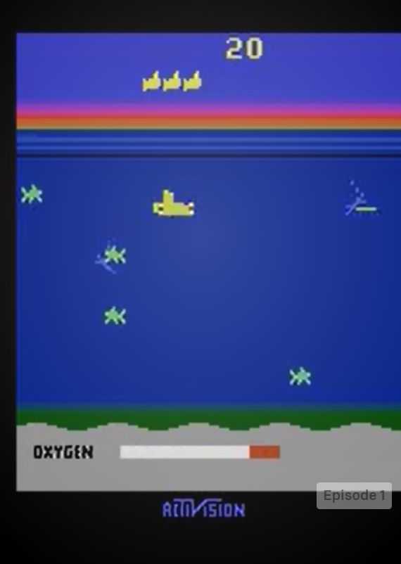
Under review as a conference paper at ICLR 2022

uncertainty scores, while in-distribution states will have relatively lower scores, therefore making
them distinguishable. This is in contrast with vanilla Q-learning algorithms that do not take into
account unknowns during training. During inference time, our OOD uncertainty estimation score
can be flexibly computed on a single deployed model without variance estimation required.
We provide theoretical guarantees that our method can improve OOD uncertainty estimation while
ensuring the convergence of ID performance (Section 4). Empirically, we demonstrate state-of-the-
art performance on six diverse environments from OpenAI gym (Brockman et al., 2016), including
Atari games (with discrete state space) and classic control task (with continuous state space). In
all environments, our method consistently achieves near-optimal OOD detection performance, out-
performing the baselines by a substantial margin. Our method can be easily plugged into existing
Q-learning algorithms including DQN (Mnih et al., 2015) and QR-DQN (Dabney et al., 2018b) and
render stronger OOD detection performance and RL safety (Section 5). Our main contributions
are summarized as follows:
       • We propose a novel Q-learning framework for improving OOD uncertainty estimation,
         which aims at mitigating the critical issue of incorrectly high Q values from OOD state
         inputs in vanilla Q-learning algorithms;
       • We provide theoretical guarantees that our regularization improves OOD detection while
         maintaining the convergence performance of ID in Q-learning;
       • Our method establishes state-of-the-art OOD detection performance on a wide range of
         RL environments, including Atari games and classic control. Extensive ablation studies are
         conducted to show the efficacy of our algorithm.

2     P RELIMINARIES AND P ROBLEM S TATEMENT
2.1   P RELIMINARIES : R EINFORCEMENT L EARNING AND Q- LEARNING

Markov decision processes (MDP). In reinforcement learning, the agent explores an environment
and maximizes the cumulative reward. Markov decision processes (MDPs) are used to model RL.
MDPs are defined by the tuples (S, A, R, T ), where S indicates the state space, A is the set of
actions, T is the transition model between states, and R is the reward model. At each timestep t, the
agent observes a state st ∈ S, chooses an action at ∈ A, receives a reward rt ∈ R, and transits to a
new state st+1 determined by T (st+1 |st , at ). The goal is to find a policy π ∈ Π : S → A, which
maximizes the discounted return over a potentially infinite horizon:
                                          Rt = Σ∞       k
                                                   k=0 γ rt+k ,                                     (1)
where γ ∈ [0, 1] is the discount factor. For notation brevity, we use s0 = st+1 and omit the timestamp
t when the context is clear.
Reinforcement learning and Q-learning. To find the optimal policy π ∗ , we focus on Q-
learning (Watkins & Dayan, 1992), a commonly used value-based approach. In Q-learning, the
action-value function Q : S × A → R describes the expected return when the agent takes action a
in state s, and then following policy π for all states afterwards. The optimal function Q∗ is defined
as:
                                    Q∗ (s, a) = max Eπ [R|s, a].                                   (2)
                                                   π

Given a tuple of one-step transition (s, a, s0 , r), we have the Bellman equation Q∗ (s, a) = r +
γ maxa0 Q∗ (s0 , a0 ) using dynamic programming. The one-step TD error is used to update Q values:
                            TD(s, a, r, s0 ) = r + γ max
                                                      0
                                                         Q(s0 , a0 ) − Q(s, a).                (3)
                                                    a
In tabular cases, a table of Q values are maintained for finite state-action pairs, and are updated
according to the TD error: Q(s, a) ← Q(s, a) + α(r + γ maxa0 Q(s0 , a0 ) − Q(s, a)), where α is the
learning rate. This can also be viewed as gradient updates that minimize the L2 norm of TD error.
Deep Q-Networks (DQN). In high-dimensional settings or when learning in continuous state-
spaces, it is common to use parameterized functions such as neural networks to approximate the
action-value function Q(s, a). We use the deep Q-networks (Mnih et al., 2015) parameterized by
θ, with corresponding action-value function Qθ . The norm of the TD error is minimized during
training to update the parameter θ.

                                                  2
Under review as a conference paper at ICLR 2022

2.2            O UT- OF - DISTRIBUTION D ETECTION IN R EINFORCEMENT L EARNING
When deploying an RL agent in open-world environments, it is paramount for the agent to detect
OOD states and refrain from taking actions according to policy π in the presence of OOD states.
Here we provide the definition of OOD states in the setting of RL.
In-distribution (ID) states. Given an environment and a learning algorithm, we can estimate the
distribution of the states encountered by the agent during training. We denote P as in-distribution.
Out-of-distribution (OOD) states. The general notion of OOD refers to inference-time inputs
which deviate substantially from the data encountered during training1 . In other words, OOD states
are unexpected and should not have occurred in the ID environment. Importantly, OOD states
should not be confused with under-explored states: the latter still belongs to ID with more epistemic
uncertainty than ID states, and are crucial for exploration (Osband et al., 2016). In contrast, OOD
states are not safe to explore, since the agent has no knowledge on such states during training. We
expect significantly lower Q values from OOD states, because unlike the underexplored states, the
agent should not be encouraged to explore OOD states.
OOD state detection. The goal of OOD detection is to define a decision function G such that:

                                            1 if s ∼ P,
                                  G(s) =
                                            0 otherwise.
In other words, the agent should be able to know what it does not know. The agent should take action
a ∼ π(s) only if s is in-distribution.

3              M ETHOD
In this section, we begin with a motivating example that existing Q-learning algorithms can produce
incorrectly high Q values for OOD states (Section 3.1). To mitigate this issue, we introduce our
proposed unknown-aware Q-learning method in Section 3.2.

3.1            A MOTIVATING EXAMPLE

Incorrectly high Q values for OOD states. Here we present a motivating example of possible
incorrect estimation of Q values for OOD states using existing Q-learning algorithms, particularly
vanilla DQN (Mnih et al., 2015) and bootstrapped DQN (Osband et al., 2016; 2018). We show
that such incorrectly high extrapolation of Q values cannot be mitigated by traditional uncertainty
estimation. For simplicity, we use the chain environment to illustrate the problem; see Figure 1 (a).
Action 0 indicates move left and Action 1 indicates move right. The start state is selected
uniformly randomly among 5 states {1, 2, 3, 4, 5}. If the agent arrives on state 0 or 6, a reward of 1
is received and the terminal is reached. Otherwise, the reward is 0.

                       i .fddsg
                        r=0                           r=1
                                                    action 1

    action 0                                                                               incorrectly high

      r=1                             r=0                          incorrectly high
       OOD Q values
    0          1   2              3         4   5              6   OOD Q values

                       the chain
                                                                                                               incorrectly
                                                                                                               high

                                                                                                               OOD Q
(a) The chain environment with                                                                                 values

states: 0,1,2,3,4,5,6.

                                                                    (b) Q values for action 0                    (c) Q values for action 1
Figure 1: The example of incorrectly high extrapolation of Q values for OOD states in the chain environment.
See Section 3.1 for details.
We train a vanilla DQN and bootstrapped DQN (with an ensemble size 10), both under the same
MLP architecture for 100,000 steps. The MLP has two hidden layers with 256 units each. Figure 1
   1
     By “inference-time”, we assume the RL agent has already converged to policy π; this policy is now fixed
and used to behave in the environment, which includes the majority of cases in RL deployment.

                                                                                       3
Under review as a conference paper at ICLR 2022

(b)(c) show the Q values for action 0 and 1 respectively. We observe that they give the same estima-
tion for in-distribution Q values, which indicates that they both achieve convergence. Vanilla DQN
fails to extrapolate reasonably on OOD states (states < 0 and > 6), where the corresponding Q val-
ues are incorrectly high. Bootstrapped DQN (Osband et al., 2016; 2018)(denoted as the ensemble
in the plots) displays higher variance for OOD state inputs, but the overall estimated distribution of
OOD Q values are still incorrectly high.
Motivated by this, we now introduce our method, which regularizes the Q values of OOD states and
improves OOD detection without compromising the in-distribution Q values; see the orange lines
shown in Figure 1 (b) and (c).

3.2    U NKNOWN - AWARE D EEP Q- LEARNING

Energy interpretation of Q-learning. In Q-learning, the agent collects data from the experience
and updates Q(s, a) for each state-action pair. We can define the probability2 p(a|s) that a is the
chosen action given the state s:
                                                          eQ(s,a)
                                           p(a|s) =                .                                         (4)
                                                         Σ eQ(s,a)
                                                         a∈A

We can rewrite p(a|s) as:
                                                   eQ(s,a)     p(s, a)
                                     p(a|s) =         Q(s,a)
                                                             =         .                                     (5)
                                                  Σ e           p(s)
                                                a∈A
Directly estimating log p(s) can be computationally intractable as it requires sampling from the
entire state space S. On the other hand, the the log of denominator, also known as the negative free
energy3 Eneg (s) = log Σ eQ(s,a) , can be easily computed from the Q values. Note that Eneg is
                           a∈A
proportional to log p(s) with some unknown factor that may depend on the state s.
The need for regularization. If Eneg (s) is smaller for OOD states than ID states, we can use Eneg (s)
for OOD detection. However, this is not guaranteed since the TD error only focuses on the Q values
for ID states, Q values for OOD states can be unbounded (see Figure 1 (b)(c)) and thus produce
incorrectly high Eneg (s) for OOD states. As a result, Eneg (s) from the vanilla Q-learning cannot be
used as an indicator of OOD states, which motivates our regularization in the following.
Energy regularization for Q-learning. We propose regularizing Q values of OOD states, which
lowers Eneg (s) for OOD states while still optimizing the performance on ID states using the standard
TD error. Recall that the original TD error as the loss in Q-learning is given by:
          E(s,a,r,s0 )∈H [TD(s, a, r, s0 )]2 = E(s,a,r,s0 )∈H [(r + γ max
                                                                       0
                                                                          Q(s0 , a0 ) − Q(s, a))2 ],         (6)
                                                                             a

where H = {(s, a, r, s0 )} is an off-policy experience replay set. To regularize the Q values of OOD
states, we add a regularization term to the original TD error, which results in the following loss:
                          L = E(s,a,r,s0 )∈H [(r + γ max
                                                      0
                                                         Q(s0 , a0 ) − Q(s, a))2 ]
                                                          a
                                                          Q(s̃,ã)
                                                                                                             (7)
                           + λEs̃∈U [(max(log Σ e                    − Eout , 0))2 ],
                                                  ã∈A

where U is the set of OOD states for training, and Eout is the energy margin hyperparameter. The
loss pulls the energy of OOD states to be lower than Eout . Details of OOD states for training are
provided in Section 5, where we show that such states can be conveniently generated using random
noises without additional datasets or environments. During inference time, we use Eneg (s) as the
uncertainty score for OOD detection, where higher Eneg (s) is classified as ID and vice versa. For
the hyperparameter Eout , a natural option is to choose Eout smaller than the lower bound of in-
distribution Eneg (s), and we also ablate the effect of hyperparameter in Section 5.3 which supports
this option.
   2
      Note that one cannot confuse p(a|s) with the policy (which is denoted as π(a|s)). Here we only use p(a|s)
to denote probability in the energy-based model to facilitate the interpretation. In Q-learning, π(a|s) is chosen
to optimize the Q values (Watkins & Dayan, 1992).
    3
      We refer readers to LeCun et al. (2006) for an extended background on the definition of free energy.

                                                         4
Under review as a conference paper at ICLR 2022

4     C ONVERGENCE G UARANTEE

In this section, we provide theoretical understandings of why our proposed regularization can
improve OOD uncertainty estimation while ensuring the ID convergence performance of the Q-
learning algorithm. For completeness, we discuss two cases separately: tabular Q-learning (Sec-
tion 4.1) and deep Q-networks (Section 4.2).

4.1   T HE TABULAR CASE

We first provide the guarantees under the tabular case, where the Q values for different state-action
pairs (s, a) are independently stored in a Q table. We expand the state space and Q table to include
the OOD state. We show that we can regularize Q values for OOD states without affecting the
convergence of in-distribution Q∗ .

Lemma 1 In the tabular case, the global minimizer of the loss function L presented in equation (7)
still satisfies Q∗ for (s, a, r, s0 ) ∈ H, and satisfies Eneg (s̃) ≤ Eout , ∀s̃ ∈ U.

Proof. We can analyze the partial derivative of in-distribution value Q(s, a), Q(s0 , a0 ) and Q(s̃, ã)
value of OOD states respectively:
                 ∂L
                        = −2P {(s, a, r, s0 ) ∈ H}(r + γ max Q(s0 , a0 ) − Q(s, a)),                (8)
               ∂Q(s, a)                                   a0

                 ∂L
                            = 2γP {(s, a, r, s0 ) ∈ H}(r + γ max Q(s0 , a0 ) − Q(s, a)),            (9)
               ∂Q(s0 , a0 )                                   a0

and
                ∂L                                                        eQ(s̃,ã)
                         = 2λP {s̃ ∈ U} max(log Σ eQ(s̃,ã) − Eout , 0)(             ).            (10)
              ∂Q(s̃, ã)                       ã∈A                      Σ eQ(s̃,ã)
                                                                               ã∈A

The loss function is convex for each Q value as independent inputs. To find the global minimum,
we only need equation (8), (9) and (10) to be zero. Note that all probabilities above are non-zero.
For equation (8) and (9) to be zero, we have that Q(s, a) = r + γ maxa0 Q(s0 , a0 ), which means
in-distribution Q values satisfy the Bellman equation and thus reach Q∗ . For equation (10) to be
zero, we have Eneg (s̃) ≤ Eout , ∀s̃ ∈ U.
Remark. To see how the Q values of OOD states are regularized, we can look at equation (10). If
the energy is larger than Eout , it would be penalized according to the scale of p(a|s). This results in
two effects: first, the Q values of OOD states would be pushed down; second, the distribution p(·|s)
would be encouraged towards a uniform distribution, which is desirable for the OOD state since the
agent should be “confused” about which action to choose under OOD states.
The tabular case is an extreme example of function approximation with perfect localization, i.e.,
each Q(s, a) can be independently optimized without affecting each other. Next, we proceed to the
DQN case, where all Q values are parameterized by a neural network.

4.2   T HE DQN CASE

We now consider the DQN case, where loss in equation (7) can be written in the following parame-
terized form: L(θ) = T (θ) + λEs̃∈U [R(θ)], where

                     T (θ) = E(s,a,r,s0 )∈H [(r + γ max
                                                     0
                                                        Qθ (s0 , a0 ) − Qθ (s, a))2 ]              (11)
                                                         a
                                                Qθ (s̃,ã)
                     R(θ) = [max(log Σ e                     − Eout , 0)]2 .                       (12)
                                         ã∈A

The next lemma shows that a local optimum of T (θ) under certain conditions is also a local mini-
mizer for L(θ) (using energy regularization). In other words, we can regularize Q values for OOD
states without affecting the convergence of in-distribution Q∗ .

                                                      5
Under review as a conference paper at ICLR 2022
Lemma 2 Assume that L(θ) and T (θ) are both twice differentiable functions. Let θ∗ be a local
minimizer of T (θ) that satisfies the sufficient conditions:
∇θ∗ T (θ∗ ) = 0,
(13)
∇2θ∗ T (θ∗ ) 0.
If θ∗ also satisfies the additional condition below:
max(log Σ eQθ∗ (s̃,ã) − Eout , 0) = 0, ∀s̃ ∈ U, (14)
ã∈A
then θ∗ is also a local minimizer of L(θ).
Proof. We can derive the first order derivative of the loss: ∇θ L(θ) = ∇θ T (θ) + λEs̃∈U [∇θ R(θ)].
Let y(θ) = ∇θ max(log Σ eQθ (s̃,ã) − Eout , 0). We have
ã∈A
∇θ R(θ) = 2λ max(log Σ eQθ (s̃,ã) − Eout , 0)y(θ). (15)
ã∈A
Plugging in the condition in equation (14), we have ∇θ∗ R(θ∗ ) = 0. So ∇θ∗ L(θ∗ ) = 0.
For the second derivative, ∇2θ L(θ) = ∇2θ T (θ) + λEs̃∈U [∇2θ R(θ)]. For ∇2θ R(θ) we have
∇2θ R(θ) = 2λ max(log Σ eQθ (s̃,ã) − Eout , 0)∇θ y(θ) + 2λy(θ)y(θ)T . (16)
ã∈A
Notice that y(θ)y(θ)T is positive semidefinite. Plugging in the condition in equation (14), we have
∇2θ∗ R(θ∗ ) < 0. Combined with ∇2θ∗ T (θ∗ ) 0, we have ∇2θ∗ L(θ∗ ) 0. Since L(θ) is twice
differentiable and θ∗ satisfies ∇θ∗ L(θ∗ ) = 0 and ∇2θ∗ L(θ∗ ) 0, θ∗ is a local optimizer of L(θ).
Remark. If we only consider the sufficient condition for a local optimizer of T (θ) (equation (13)),
leaving the OOD Q values unbounded, there are multiple solutions with the same in-distribution Q
values and different OOD Q values. From universal approximation theorems, the more hidden units
the neural network has, the more representation power it possesses. It is therefore easy to find θ∗
that satisfies both equation (13) and (14). A visualization of such solutions can be found in Figure 1
(b) and (c), showing that our regularization on DQN can only affect OOD Q values without affecting
the convergence of in-distribution values.
5 E XPERIMENTS
In this section, we describe our experimental setup (Section 5.1) and demonstrate the effectiveness of
our method on several OOD evaluation tasks (Section 5.2). We also conduct extensive ablation stud-
ies and comparative analyses that lead to an improved understanding of our method (Section 5.3).
5.1 S ETUP
Environments. To systematically evaluate our approach, we benchmark on a variety of environ-
ments, including Atari games (with discrete state space) and a classic control task (with continuous
state space) in OpenAI gym (Brockman et al., 2016). These environments allow assessing OOD
states in a controlled and reproducible way. For Atari games, we choose five most commonly used
environments: Pong, Breakout, Seaquest, Qbert and RoadRunner. We provide sample
pictures of the states in each environment in Appendix E. In addition, we also evaluate a classic
control task, Cartpole-v0 from OpenAI gym (Brockman et al., 2016), where the goal is to prevent a
pole from falling over a moving cart. Due to space constraints, we present results on Atari games in
the main paper (Section 5.2) and we refer readers to the Appendix Section F for results on Cartpole,
where our method consistently displays strong performance.
Training. Our method can be directly compatible with existing Q-learning algorithms. In particular,
we consider two commonly used methods: vanilla DQN(Mnih et al., 2015) and QR-DQN(Dabney
et al., 2018b). We add the regularization term to the loss function in training as shown in equation
7. The regularization weight λ = 0.01 and Eout = 0 for DQN and λ = 0.001 and Eout = 0 for QR-
DQN in all environments. Hyperparameters for DQN and QR-DQN can be found in Appendix A,
6Under review as a conference paper at ICLR 2022
ID Env Method\OOD Env Breakout Seaquest Qbert RoadRunner
FPR95 ↓ AUROC ↑ FPR95 ↓ AUROC ↑ FPR95 ↓ AUROC ↑ FPR95 ↓ AUROC ↑
DQN 97.57 30.29 56.50 81.50 49.21 92.26 99.57 3.72
A2C 19.15 94.85 32.38 84.81 63.56 73.19 0.69 99.41
Pong PPO 0.11 99.95 16.16 90.45 0.00 100.00 0.24 99.97
Ensemble (10 NNs) 0.00 99.94 0.03 99.89 0.00 100.00 0.00 100.00
Ours 0.00 100.00 0.14 99.92 0.00 100.00 0.00 100.00
Method\Test Env Pong Seaquest Qbert RoadRunner
FPR95 ↓ AUROC ↑ FPR95 ↓ AUROC ↑ FPR95 ↓ AUROC ↑ FPR95 ↓ AUROC ↑
DQN 100.00 24.85 99.85 30.84 100.00 27.19 100.00 34.98
A2C 100.00 47.08 98.04 60.67 98.87 81.90 73.93 79.68
Breakout PPO 74.72 81.89 94.69 74.46 72.28 91.08 48.02 86.33
Ensemble (10 NNs) 99.76 74.04 23.68 96.09 30.20 94.87 59.54 91.85
Ours 0.15 99.99 0.15 99.99 0.00 100.00 2.91 98.28
Method\Test Env Pong Breakout Qbert RoadRunner
FPR95 ↓ AUROC ↑ FPR95 ↓ AUROC ↑ FPR95 ↓ AUROC ↑ FPR95 ↓ AUROC ↑
DQN 100.00 94.79 77.31 93.42 95.94 82.89 99.81 54.21
A2C 100.00 81.53 100.00 77.76 100.00 85.73 99.77 88.78
Seaquest PPO 100.00 94.19 94.72 93.24 99.97 91.36 99.70 87.89
Ensemble (10 NNs) 0.00 99.82 0.00 99.85 0.03 99.68 0.00 99.85
Ours 0.00 100.00 0.00 100.00 0.00 100.00 0.00 100.00
Method\Test Env Pong Breakout Seaquest RoadRunner
FPR95 ↓ AUROC ↑ FPR95 ↓ AUROC ↑ FPR95 ↓ AUROC ↑ FPR95 ↓ AUROC ↑
DQN 92.62 89.43 94.53 37.09 99.85 25.76 99.90 0.71
A2C 0.94 99.20 46.08 90.59 68.16 89.89 99.87 56.21
Qbert PPO 38.43 95.05 27.88 96.50 2.87 99.08 96.40 73.99
Ensemble (10 NNs) 99.97 50.30 72.30 70.76 94.91 56.80 90.28 66.58
Ours 0.00 100.00 0.00 100.00 0.00 100.00 0.00 100.00
Method\Test Env Pong Breakout Seaquest Qbert
FPR95 ↓ AUROC ↑ FPR95 ↓ AUROC ↓ FPR95 ↓ AUROC ↑ FPR95 ↓ AUROC ↑
DQN 100.00 88.90 99.99 88.59 100.00 87.54 100.00 88.69
A2C 100.00 57.74 100.00 66.64 99.93 77.14 100.00 65.96
RoadRunner PPO 100.00 87.95 99.99 86.98 99.95 83.06 100.00 88.16
Ensemble (10 NNs) 23.08 95.98 0.08 99.92 14.18 96.85 0.35 99.72
Ours 0.00 100.00 0.00 100.00 0.00 100.00 0.00 100.00
Table 1: FPR95 and AUROC on Atari games. Superior results are marked in bold. A2C, PPO, Vanilla
DQN, Ensemble (Bootstrapped DQN with randomized prior functions, ensemble size = 10) are baselines for
comparison.
and we maintain the same set of DQN parameters for both vanilla DQN and our method. We train
the agent for 100,000 steps for Cartpole, and 10 million steps for Atari games.
Baselines. We compare our approach with various competitive baselines in literature: the first group
of baselines are vanilla value-based learning algorithms: A2C (Mnih et al., 2016), PPO (Schulman
et al., 2017), and vanilla DQN (Mnih et al., 2015). Another baseline is the ensemble-based Q-
learning algorithm Bootstrapped DQN (Osband et al., 2016; 2018), which is used for OOD detection
in Sedlmeier et al. (2019) and Hoel et al. (2020). Specifically, we use the variance of Q values for
OOD score as in Sedlmeier et al. (2019) and Hoel et al. (2020). Specifically, the detection score
is based on −Var[Q(s, amax )], where amax = arg maxa∈A Q(s, a) is the action performed after
convergence of training. The variance is estimated on an ensemble of 10 neural networks, same
as in Sedlmeier et al. (2019) and Hoel et al. (2020). For value-based learning algorithms, we use
Eneg (s) as the score for OOD detection in vanilla DQN, and V (s) in A2C and PPO since they
maintain value function instead of Q function during learning4 .
Evaluation metrics. We measure the following metrics that are commonly used for OOD detection:
(1) the false positive rate (FPR95) of OOD examples when the true positive rate of in-distribution
examples is at 95%, and (2) the area under the receiver operating characteristic curve (AUROC). For
ID evaluation, we also report the cumulative reward of the agent.
5.2 E XPERIMENTAL RESULTS
OOD states for training and test. For agents trained on each of the 5 Atari environments, we
use states generated from the other four environments as test-time OOD states since the states of
Atari games are of the same shape and pixel range. For neural network inputs, observations are
preprocessed into W × W × 4 grayscale frames as in Mnih et al. (2015). To create the training-time
OOD states s̃ ∈ U, we randomly crop a square of the ID states and replace the pixels with uniform
4
The entropy in A2C and PPO can also be used for OOD detection. However, we show in Appendix G that
they do not produce desirable OOD detection results.
7Under review as a conference paper at ICLR 2022
(a) Pong (b) Breakout (c) Seaquest (d) Qbert (e) RoadRunner
Figure 2: Learning curves of vanilla DQN (blue) vs. energy-regularized DQN (orange) for Atari games. Full
curves of DQN, QR-DQN and the comparison of regularized versions are presented in Appendix D.
random pixels in [0, 255]. The cropping width is selected uniformly between [α · W, W ], where
α = 1/4. An ablation study on the effect of cropping size and location is provided in Section 5.3.
Detection results. In Table 1, we show comparisons in a series of high-dimensional Atari environ-
ments with image inputs. Our method outperforms vanilla DQN, A2C, PPO, and ensemble-based
method (Bootstrapped DQN). Moreover, Bootstrapped DQN requires deploying an ensemble of
RL agents to estimate the uncertainty, which can be computationally expensive as the inference
time increases with ensemble size. In contrast, our method does not incur any additional computa-
tion overhead during inference time compared with vanilla DQN. In all environments, our method
achieves near-optimal performance (e.g., 0 FPR95). Additional results on QR-DQN are in Appendix
C, where our method shows consistent improvement over vanilla QR-DQN.
Convergence performance and learning curves. We further show that our method improves OOD
detection while ensuring the convergence performance for the in-distribution environment. Our em-
pirical observation justifies the theoretical insights in Section 4.2, where we show regularizing the
Q values of OOD states does not affect the convergence performance of ID. Specifically, Figure 2
shows the learning curves for each Atari environment. We contrast the learning curves of vanilla
DQN and our regularized version since they share the same policy and only differ in the regular-
ization term. In most environments like Pong, the convergence performance is comparable before
and after regularization. In Seaquest where the vanilla DQN gets stuck in a suboptimal policy,
our regularization helps to escape from the suboptimal and converges faster to a better policy, which
shows the effect that correcting the wrong extrapolation in OOD spaces can potentially help to learn
the correct ID Q values. The final rewards of the ID environment can be found in Table 2, where
our method shows comparable or better results than vanilla DQN. Our method has a similar regular-
ization effect on QR-DQN that displays similar or better convergence. Learning curves of QR-DQN
and energy-regularized QR-DQN, together with final rewards can be found in Appendix D.
Method Pong Breakout Seaquest Qbert RoadRunner
Vanilla DQN 20.8 ± 0.4 350.0 ± 51.0 2056.0 ± 601.0 9950.0 ± 4807.5 37070.0 ± 5256.8
Ours 20.7 ± 0.8 377.8 ± 20.1 2816.0 ± 621.8 9496.0 ± 5061.3 40600.0 ± 8881.8
Table 2: Final rewards of DQN and our regularized DQN (averaged over 10 evaluations).
5.3 A BLATION S TUDY ON H YPERPARAMETERS IN R EGULARIZATION
In this subsection, we ablate the effect of each hyperparameter in our regularization: margin Eout ,
regularization weight λ, crop width and location, and noise type. For this ablation, we use Pong as
the ID, remainder 4 environments as OOD, and another Atari game SpaceInvader for validation.
Below we summarize our key findings. The complete results can be found in Appendix B.
(1) Energy margin Eout : We vary the values of Eout in [−10, 10]. Note that all rewards encountered
in Atari games are above zero, the lower bound of energy value for ID states is 0. We test values
both higher and lower than 0 to show the effect comprehensively. As shown in Table 4 in Appendix
B, our method is not sensitive to the hyperparameter as long as Eout ≤ 0. In particular, positive Eout
leads to less distinguishable energy distributions between ID and OOD states.
(2) Regularization weight λ: We vary the weights from 0.001 to 0.5, where we show the OOD
detection results are not sensitive to the weight parameter (see Table 5 in Appendix).
(3) Cropping size: As we mentioned in Section 5.2, we crop a random square on the original
ID input of size W × W and replace it with random noise to construct OOD states for training.
Here the crop width and height are randomly chosen from [α · W, W ]. We ablate on the effect of
α ∈ [1/8, 2/8, ..., 7/8]. As seen in Table 6 in Appendix, the results are not very sensitive to α except
for when it is too small. It is expected since such states can be similar to ID under a small α.
8Under review as a conference paper at ICLR 2022
(4) Cropping location: As shown in Table 7 in Appendix, random cropping location yields the most
diverse OOD training states. We contrast this with alternatives using fixed locations, and show that
random location leads to better performance due to more data diversity.
(5) Noise type: We evaluate different types of noise: uniform and Gaussian. For Gaussian noise,
we add N (0, 1) i.i.d. noise to the normalized image. Table 8 in Appendix show that both ID reward
and OOD detection performance are not sensitive to noise types.
6 R ELATED WORKS
OOD uncertainty estimation in supervised learning. The phenomenon of neural networks’ over-
confidence in out-of-distribution data is revealed by Nguyen et al. (2015). Early works attempt to
improve the OOD uncertainty estimation by proposing the ODIN score (Liang et al., 2018), ensem-
ble method (Lakshminarayanan et al., 2017), and Mahalanobis distance-based confidence score (Lee
et al., 2018). Recent work by Liu et al. proposed using an energy score for OOD uncertainty es-
timation, which demonstrated advantages over the softmax confidence score. Different from the
classification model, our work focuses on an underexplored setting Q-learning, where the Q values
are regressed according to the TD error, rather than cross-entropy loss which does not bound the
exact logit values. In addition, we provide new theoretical guarantees which explain rigorously that
our training objective does not affect the convergence of the Q-learning (for both tabular and DQN
cases). Moreover, while works in the supervised learning setting may require auxiliary outlier data
sets for model regularization (Hendrycks et al., 2018; Mohseni et al., 2020), our work shows that a
more general and flexible solution of generating random OOD states can be effective in RL.
Uncertainty estimation in deep Q learning. The problem of OOD detection in RL remains largely
untapped. Recently, Sedlmeier et al. (2019); Hoel et al. (2020) employed ensemble-based uncer-
tainty estimation for OOD detection, which serves as a strong baseline. Variational inference meth-
ods in deep Q-learning as epistemic uncertainty estimation is also explored for OOD detection:
Sedlmeier et al. (2019) compared MC-dropout (Kendall & Gal, 2017; Gal et al., 2017) with DQN
and show that MC-dropout does not yield viable results. For this reason, we omit it in the baselines.
Other works in epistemic estimation for Q-learning, such as Bayesian modeling (Azizzadenesheli
et al., 2018), information-directed sampling (Nikolov et al., 2018) and randomized value function
(Touati et al., 2020) also do not fundamentally mitigate the issue of incorrectly high Q values in
the presence of OOD inputs in Section 3.1. A separate line of works quantifies the aleatoric uncer-
tainty in Q-learning (Tamar et al., 2016; Bellemare et al., 2017; Dabney et al., 2018a). However,
aleatoric uncertainty is not suitable for OOD detection, since it focuses on the internal distribution
of the ID environment. Our method is also orthogonal and complementary to methods that focus on
improving the ID performance of Q-learning (including QR-DQN that we considered).
OOD actions in offline RL. In offline RL, the agent is trained with a constrained set of historical
data instead of interacting with the real environment. Current literature focuses on the issue of action
distribution shift between the policy used to obtain the historical data and the learned policy, which
results in bootstrapping errors and leads to failure in training. Various methods have been proposed
to mitigate this issue (Kumar et al., 2019; 2020; Argenson & Dulac-Arnold, 2020; Kostrikov et al.,
2021). Our focus is different, where we detect distribution shifts in the state space in deployment,
rather than shifts in action space during offline training.
7 C ONCLUSION AND O UTLOOK
In this work, we propose an unknown-aware deep Q-learning framework for detecting out-of-
distribution states in open-world RL deployment—an important yet underexplored problem. We
show that energy regularization during Q-learning can effectively mitigate the issue of incorrectly
high extrapolation of Q values for OOD states, and as a result, lead to strong separability between
ID and OOD states in deployment. We provide theoretical guarantees, provably showing that our
method can ensure the convergence performance of the ID environment while improving OOD de-
tection. Empirically, our method establishes state-of-the-art OOD detection performance on diverse
environments including Atari games and classic control. We hope our work will increase the re-
search awareness and inspire future research toward a broader view of OOD uncertainty estimation
for deep reinforcement learning.
9Under review as a conference paper at ICLR 2022
R EPRODUCIBILITY S TATEMENT
The authors of the paper are committed to reproducible research. Below we summarize our efforts
that facilitate reproducible results:
1. Environments. We use publicly available RL environments from OpenAI gym, which are
described in detail in Section 5.1.
2. Assumption and proof. The complete proof of our theoretical contribution is provided in
Section 4, which supports our theoretical claims made in Lemma 1 and Lemma 2.
3. RL training. We follow the original implementation in Raffin (2020) for DQN and QR-
DQN. Details of training configurations are fully summarized in Appendix A (Table 3).
4. Hyperparameters of our method. The hyperparameters used in energy regularization are
described in Section 5.1. We also ablate the effect of each hyperparameter in our method,
and provide results in Section 5.3 and Appendix B.
5. Baselines. The description of baseline methods and hyperparameters are specified in Sec-
tion 5.1 and Appendix A.
6. Open source code. The codebase will be publicly released for reproducible research. As
a reference, we will also attach the code in OpenReview (visible to ACs and reviewers on
the discussion forum).
10Under review as a conference paper at ICLR 2022
R EFERENCES
Arthur Argenson and Gabriel Dulac-Arnold. Model-based offline planning. In International Con-
ference on Learning Representations, 2020.
Kamyar Azizzadenesheli, Emma Brunskill, and Animashree Anandkumar. Efficient exploration
through bayesian deep q-networks. In 2018 Information Theory and Applications Workshop (ITA),
pp. 1–9. IEEE, 2018.
Marc G Bellemare, Will Dabney, and Rémi Munos. A distributional perspective on reinforcement
learning. In International Conference on Machine Learning, pp. 449–458. PMLR, 2017.
Greg Brockman, Vicki Cheung, Ludwig Pettersson, Jonas Schneider, John Schulman, Jie Tang, and
Wojciech Zaremba. Openai gym. arXiv preprint arXiv:1606.01540, 2016.
Will Dabney, Georg Ostrovski, David Silver, and Rémi Munos. Implicit quantile networks for
distributional reinforcement learning. In International conference on machine learning, pp. 1096–
1105. PMLR, 2018a.
Will Dabney, Mark Rowland, Marc G Bellemare, and Rémi Munos. Distributional reinforcement
learning with quantile regression. In Thirty-Second AAAI Conference on Artificial Intelligence,
2018b.
Yarin Gal, Jiri Hron, and Alex Kendall. Concrete dropout. Advances in Neural Information Pro-
cessing Systems, 30, 2017.
Dan Hendrycks, Mantas Mazeika, and Thomas Dietterich. Deep anomaly detection with outlier
exposure. In International Conference on Learning Representations, 2018.
Carl-Johan Hoel, Tommy Tram, and Jonas Sjöberg. Reinforcement learning with uncertainty esti-
mation for tactical decision-making in intersections. In 2020 IEEE 23rd International Conference
on Intelligent Transportation Systems (ITSC), pp. 1–7. IEEE, 2020.
Alex Kendall and Yarin Gal. What uncertainties do we need in bayesian deep learning for computer
vision? Advances in Neural Information Processing Systems, 30:5574–5584, 2017.
Ilya Kostrikov, Rob Fergus, Jonathan Tompson, and Ofir Nachum. Offline reinforcement learning
with fisher divergence critic regularization. In International Conference on Machine Learning,
pp. 5774–5783. PMLR, 2021.
Aviral Kumar, Justin Fu, Matthew Soh, George Tucker, and Sergey Levine. Stabilizing off-policy q-
learning via bootstrapping error reduction. Advances in Neural Information Processing Systems,
32:11784–11794, 2019.
Aviral Kumar, Aurick Zhou, George Tucker, and Sergey Levine. Conservative q-learning for offline
reinforcement learning. arXiv preprint arXiv:2006.04779, 2020.
Balaji Lakshminarayanan, Alexander Pritzel, and Charles Blundell. Simple and scalable predic-
tive uncertainty estimation using deep ensembles. In Advances in neural information processing
systems, pp. 6402–6413, 2017.
Yann LeCun, Sumit Chopra, Raia Hadsell, M Ranzato, and F Huang. A tutorial on energy-based
learning. Predicting structured data, 1(0), 2006.
Kimin Lee, Kibok Lee, Honglak Lee, and Jinwoo Shin. A simple unified framework for detecting
out-of-distribution samples and adversarial attacks. In Advances in Neural Information Process-
ing Systems, pp. 7167–7177, 2018.
Shiyu Liang, Yixuan Li, and Rayadurgam Srikant. Enhancing the reliability of out-of-distribution
image detection in neural networks. In 6th International Conference on Learning Representations,
ICLR 2018, 2018.
Weitang Liu, Xiaoyun Wang, John Owens, and Yixuan Li. Energy-based out-of-distribution detec-
tion. Advances in Neural Information Processing Systems, 2020.
11Under review as a conference paper at ICLR 2022
Volodymyr Mnih, Koray Kavukcuoglu, David Silver, Andrei A Rusu, Joel Veness, Marc G Belle-
mare, Alex Graves, Martin Riedmiller, Andreas K Fidjeland, Georg Ostrovski, et al. Human-level
control through deep reinforcement learning. nature, 518(7540):529–533, 2015.
Volodymyr Mnih, Adria Puigdomenech Badia, Mehdi Mirza, Alex Graves, Timothy Lillicrap, Tim
Harley, David Silver, and Koray Kavukcuoglu. Asynchronous methods for deep reinforcement
learning. In Maria Florina Balcan and Kilian Q. Weinberger (eds.), Proceedings of The 33rd
International Conference on Machine Learning, volume 48 of Proceedings of Machine Learning
Research, pp. 1928–1937, New York, New York, USA, 20–22 Jun 2016. PMLR. URL https:
//proceedings.mlr.press/v48/mniha16.html.
Sina Mohseni, Mandar Pitale, JBS Yadawa, and Zhangyang Wang. Self-supervised learning for
generalizable out-of-distribution detection. In Proceedings of the AAAI Conference on Artificial
Intelligence, pp. 5216–5223, 2020.
Anh Nguyen, Jason Yosinski, and Jeff Clune. Deep neural networks are easily fooled: High confi-
dence predictions for unrecognizable images. In Proceedings of the IEEE conference on computer
vision and pattern recognition, pp. 427–436, 2015.
Nikolay Nikolov, Johannes Kirschner, Felix Berkenkamp, and Andreas Krause. Information-
directed exploration for deep reinforcement learning. In International Conference on Learning
Representations, 2018.
Ian Osband, Charles Blundell, Alexander Pritzel, and Benjamin Van Roy. Deep exploration via
bootstrapped dqn. Advances in neural information processing systems, 29:4026–4034, 2016.
Ian Osband, John Aslanides, and Albin Cassirer. Randomized prior functions for deep reinforcement
learning. Advances in Neural Information Processing Systems, 31, 2018.
Antonin Raffin. Rl baselines3 zoo. https://github.com/DLR-RM/
rl-baselines3-zoo, 2020.
John Schulman, Filip Wolski, Prafulla Dhariwal, Alec Radford, and Oleg Klimov. Proximal policy
optimization algorithms. arXiv preprint arXiv:1707.06347, 2017.
Andreas Sedlmeier, Thomas Gabor, Thomy Phan, Lenz Belzner, and Claudia Linnhoff-Popien.
Uncertainty-based out-of-distribution classification in deep reinforcement learning. arXiv preprint
arXiv:2001.00496, 2019.
Aviv Tamar, Dotan Di Castro, and Shie Mannor. Learning the variance of the reward-to-go. The
Journal of Machine Learning Research, 17(1):361–396, 2016.
Ahmed Touati, Harsh Satija, Joshua Romoff, Joelle Pineau, and Pascal Vincent. Randomized value
functions via multiplicative normalizing flows. In Uncertainty in Artificial Intelligence, pp. 422–
432. PMLR, 2020.
Christopher JCH Watkins and Peter Dayan. Q-learning. Machine learning, 8(3-4):279–292, 1992.
12Under review as a conference paper at ICLR 2022
A H YPERPARAMETERS OF RL T RAINING
We follow the original implementation in Raffin (2020) for DQN and QR-DQN. We maintain the
same hyperparameters from their implementation for both original vs. our regularized networks.
Details of hyperparameters used in DQN and QR-DQN are as follows:
Parameters DQN (Cartpole) QR-DQN (Cartpole) DQN (Atari) QR-DQN (Atari)
Network architecture MLP 5 MLP 6 CNN7 CNN 8
Buffer size 100000 100000 10000 10000
Learning rate 2.3e-3 2.3e-3 1e-4 1e-4
Batch size 64 64 32 32
Steps to start learning 1000 1000 100000 100000
Target update interval 10 10 1000 1000
Training frequency 256 256 4 4
Gradient step 128 128 1 1
Exploration fraction 0.16 0.16 0.1 0.025
Final probability of random actions 0.04 0.04 0.01 0.01
Table 3: Hyparameters for DQN and QR-DQN in each environment.
For the ensemble-based method, we maintain the common hyperparameter from DQN, and follow
https://github.com/johannah/bootstrap_dqn for hyperparameters of Bootstrapped
DQN. For A2C and PPO, we use the same hyperparameters as Raffin (2020).
B F ULL A BLATION R ESULTS ON H YPERPARAMETERS IN R EGULARIZATION
Here we present the full ablation results and final rewards of ID performance. The training envi-
ronment is Pong. While ablating each hyperparameter, we keep others unchanged. Note that for
Pong, the highest cumulative reward for ID evaluation is 21.
(1) Ablation on energy margin Eout : We vary the values of Eout in [−10, 10]. Note that all rewards
encountered in Atari games are above zero, the lower bound of energy value for ID states is 0.
We vary Eout to be both higher and lower than 0 and show the effect comprehensively. As shown in
Table 4, our method is not sensitive to the hyperparameter as long as Eout ≤ 0. In particular, positive
Eout leads to less distinguishable energy distributions between ID and OOD states.
ID: Pong Breakout Seaquest Qbert RoadRunner Validation ID reward
Eout FPR95 ↓ AUROC ↑ FPR95 ↓ AUROC ↑ FPR95 ↓ AUROC ↑ FPR95 ↓ AUROC ↑ FPR95 ↓ AUROC ↑
-10 0.00 100.00 0.33 99.81 0.00 100.00 0.00 100.00 4.42 98.31 19.60
-5 0.00 100.00 0.15 99.95 0.00 100.00 0.00 100.00 0.34 99.86 20.70
-1 0.00 100.00 0.14 99.92 0.00 100.00 0.00 100.00 1.20 99.59 20.60
0 0.00 100.00 0.00 100.00 0.00 100.00 0.00 100.00 1.22 99.55 20.70
1 0.00 100.00 0.00 100.00 0.00 100.00 0.00 100.00 3.43 99.09 19.90
5 6.33 98.25 26.50 93.46 31.46 96.01 45.78 85.45 58.37 92.43 20.80
10 33.06 94.21 21.17 93.94 0.00 100.00 63.64 74.41 45.73 92.81 20.70
Table 4: Ablation study on the energy margin Eout . Our method is not sensitive when Eout ≤ 0 in Atari games.
(2) Ablation on regularization weight λ: We vary the weights from 0.001 to 0.5, where we show
the OOD detection results are not sensitive to the weight parameter (see Table 5).
5
MLP with 2 hidden layers; 256 units for each hidden layer.
6
MLP with 2 hidden layers; 256 units for each hidden layer; number of quantiles = 25.
7
The same CNN structure as in Mnih et al. (2015).
8
The same CNN structure as in Mnih et al. (2015); number of quantiles = 200.
13Under review as a conference paper at ICLR 2022
ID: Pong Breakout Seaquest Qbert RoadRunner Validation ID reward
λ FPR95 ↓ AUROC ↑ FPR95 ↓ AUROC ↑ FPR95 ↓ AUROC ↑ FPR95 ↓ AUROC ↑ FPR95 ↓ AUROC ↑
0.5 0.00 100.00 0.40 99.95 0.00 100.00 0.00 100.00 2.26 99.29 20.60
0.1 0.00 100.00 0.00 100.00 0.00 100.00 0.00 100.00 1.06 99.67 20.70
0.05 0.00 100.00 0.00 100.00 0.00 100.00 0.00 100.00 0.31 99.93 20.30
0.01 0.00 100.00 0.14 99.92 0.00 100.00 0.00 100.00 1.20 99.59 20.60
0.005 0.00 100.00 0.00 100.00 0.00 100.00 0.00 100.00 2.51 99.25 20.30
0.001 0.00 100.00 0.48 99.95 0.00 100.00 0.00 100.00 0.35 99.86 19.50
Table 5: Ablation study on the regularization weight λ. Our detection results are not sensitive to λ.
(3) Ablation on crop width: As we mentioned in Section 5, we crop a random square on the
original ID input of size W × W and replace it with random noise to construct OOD states for
training. Here the crop width and height are randomly chosen from [α · W, W ]. We ablate on the
effect of α ∈ [1/8, 2/8, ..., 7/8]. As seen in Table 6, the results are not very sensitive to α except
for when it is too small (e.g., 1/8). It is expected since the resulting input can be similar to ID under
a small α.
ID: Pong Breakout Seaquest Qbert RoadRunner Validation ID reward
α FPR95 ↓ AUROC ↑ FPR95 ↓ AUROC ↑ FPR95 ↓ AUROC ↑ FPR95 ↓ AUROC ↑ FPR95 ↓ AUROC ↑
1/8 0.00 100.00 0.00 100.00 0.00 100.00 0.00 100.00 0.00 100.00 19.60
1/4 0.00 100.00 0.14 99.92 0.00 100.00 0.00 100.00 0.00 100.00 20.60
3/8 0.10 99.97 0.00 99.99 0.00 100.00 0.00 100.00 1.05 99.71 20.70
1/2 4.19 98.67 0.45 99.72 0.00 100.00 0.28 99.96 5.68 98.11 20.00
5/8 1.04 99.77 2.85 99.18 0.00 100.00 0.21 99.91 8.99 97.44 20.20
3/4 0.03 99.93 5.91 98.64 0.00 100.00 0.17 99.96 11.49 96.38 20.50
7/8 0.00 100.00 0.30 99.95 0.00 100.00 0.13 99.93 4.83 98.68 20.20
Table 6: Ablation study on the cropping width.
(4) Ablation on crop location: As shown in Table 7, random cropping location yields the most
diverse OOD training states. We contrast this with alternatives using fixed locations, and show that
random location leads to better performance overall.
ID: Pong Breakout Seaquest Qbert RoadRunner Validation ID reward
Crop Location FPR95 ↓ AUROC ↑ FPR95 ↓ AUROC ↑ FPR95 ↓ AUROC ↑ FPR95 ↓ AUROC ↑ FPR95 ↓ AUROC ↑
Lower left 1.80 99.28 0.67 99.69 0.00 100.00 0.51 99.76 7.12 97.61 20.60
Lower right 0.15 99.99 0.30 99.91 0.00 100.00 63.10 60.40 11.18 96.69 20.50
Middle 6.42 98.69 3.12 99.21 0.00 100.00 0.79 99.68 17.09 97.41 18.90
Upper left 0.15 99.86 25.60 92.93 0.01 100.00 65.99 57.02 13.62 96.30 20.60
Upper right 16.50 94.09 1.76 99.44 0.00 100.00 46.22 62.69 8.74 97.39 20.00
Random 0.00 100.00 0.14 99.92 0.00 100.00 0.00 100.00 0.00 100.00 20.60
Table 7: Effect of the crop location to inject OOD pixels. Random cropping yields the most desirable results.
(5) Ablation on noise types: We evaluate different types of noise: uniform and Gaussian. For
Gaussian noise, we add N (0, 1) i.i.d. noise to the normalized image. Table 8 shows that both ID
reward and OOD detection performance are not sensitive to noise types.
ID: Pong Breakout Seaquest Qbert RoadRunner Validation ID reward
Noise type FPR95 ↓ AUROC ↑ FPR95 ↓ AUROC ↑ FPR95 ↓ AUROC ↑ FPR95 ↓ AUROC ↑ FPR95 ↓ AUROC ↑
Uniform 0.00 100.00 0.14 99.92 0.00 100.00 0.00 100.00 0.00 100.00 20.60
Gaussian 0.00 100.00 0.76 99.71 0.00 100.00 0.00 100.00 1.49 99.41 20.50
Table 8: Effect of different noise types. Gaussian and uniform noises give similar results.
C OOD DETECTION RESULTS ON QR-DQN IN ATARI GAMES
Here we present the OOD detection results in Table 9 when we apply the regularization term to
another common Q-learning algorithm QR-DQN (Dabney et al., 2018b), where our method also
shows significant improvement with near-optimal results.
14Under review as a conference paper at ICLR 2022
ID Env Method\OOD Env Breakout Seaquest Qbert RoadRunner
FPR95 ↓ AUROC ↑ FPR95 ↓ AUROC ↑ FPR95 ↓ AUROC ↑ FPR95 ↓ AUROC ↑
QR-DQN 5.28 97.88 64.52 64.84 100.00 99.97 79.69 75.17
Pong
Ours (QRDQN) 0.00 100.00 0.00 100.00 0.00 100.00 0.00 100.00
Method\Test Env Pong Seaquest Qbert RoadRunner
FPR95 ↓ AUROC ↑ FPR95 ↓ AUROC ↑ FPR95 ↓ AUROC ↑ FPR95 ↓ AUROC ↑
QR-DQN 90.08 91.96 94.43 75.42 99.86 73.09 79.69 75.17
Breakout
Ours (QRDQN) 0.06 99.99 0.01 100.00 0.90 99.85 0.00 100.00
Method\Test Env Pong Breakout Qbert RoadRunner
FPR95 ↓ AUROC ↑ FPR95 ↓ AUROC ↑ FPR95 ↓ AUROC ↑ FPR95 ↓ AUROC ↑
QR-DQN 100.00 90.08 99.95 88.13 99.57 90.54 79.69 75.17
Seaquest
Ours (QRDQN) 0.00 100.00 0.00 100.00 0.00 100.00 0.00 100.00
Method\Test Env Pong Breakout Seaquest RoadRunner
FPR95 ↓ AUROC ↑ FPR95 ↓ AUROC ↑ FPR95 ↓ AUROC ↑ FPR95 ↓ AUROC ↑
QR-DQN 100.00 73.02 100.00 69.00 99.64 56.17 79.69 75.17
Qbert
Ours (QRDQN) 0.00 100.00 0.00 100.00 0.00 100.00 0.00 100.00
Method\Test Env Pong Breakout Seaquest Qbert
FPR95 ↓ AUROC ↑ FPR95 ↓ AUROC ↓ FPR95 ↓ AUROC ↑ FPR95 ↓ AUROC ↑
QR-DQN 100.00 73.02 100.00 69.00 99.64 56.17 79.69 75.17
RoadRunner
Ours (QRDQN) 0.00 100.00 0.00 100.00 0.00 100.00 0.00 100.00
Table 9: FPR95 and AUROC on Atari games. We compare the performance of QR-DQN and QR-DQN with
regularization (Ours).
D E VALUATION ON FINAL REWARD AND FULL LEARNING CURVES IN ATARI
GAMES
Here we present the final rewards of QRDQN and our regularized DQN in Table 10, where our
method also maintains a similar ID performance compared to vanilla QR-DQN.
Method Pong Breakout Seaquest Qbert RoadRunner
QR-DQN 20.2 ± 1.2 412.4 ± 159.4 2580.0 ± 26.9 14682.0 ± 479.2 43150.0 ± 7636.1
Ours (QR-DQN) 20.4 ± 0.9 406.5 ± 32.3 5060.0 ± 392.9 14965.0 ± 53.6 47930.0 ± 7870.0
Table 10: Final rewards of QR-DQN and our regularized QR-DQN (averaged over 10 evaluations).
We present the learning curves of QR-DQN and our regularized version in five Atari games in
Figure 3. Combined with final rewards in Table 10, we show that our regularization also maintains
the similar ID reward while improving the OOD detection performance, or even help the agent to
achieve better ID performance (e.g., Seaquest).
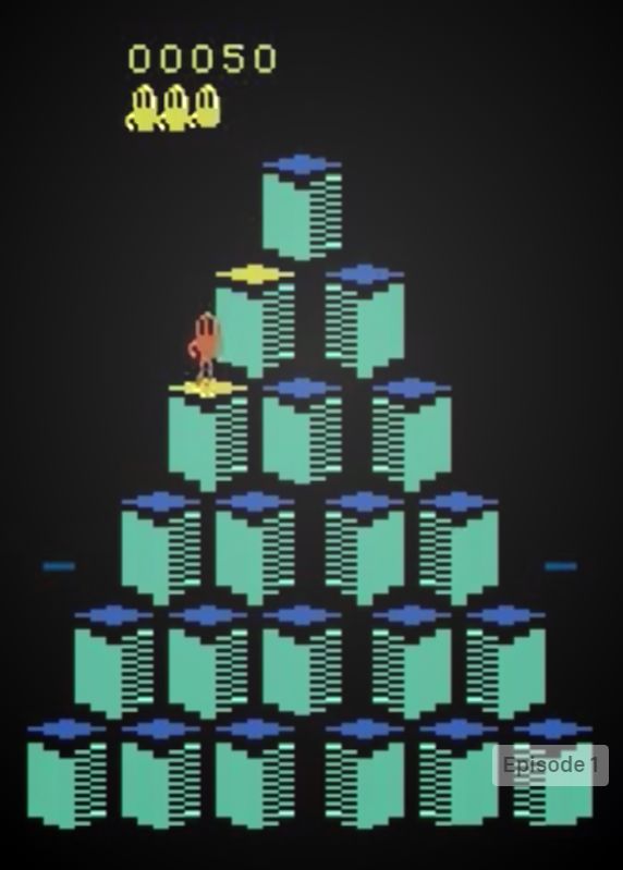
E S AMPLE PICTURES OF STATES FROM ATARI GAMES
(a) Pong (b) Breakout (c) Seaquest (d) Qbert (e) RoadRunner
F C LASSIC CONTROL TASK : C ARTPOLE
OOD states for training and test. The state space of Cartpole is a four-dimension vector, each
specifying the physical property with the following meaning and range: Cart position [−4.8, 4.8],
15Under review as a conference paper at ICLR 2022
(a) (b)
(c) (d)
(e)
Figure 3: Learning curves of QR-DQN vs ours with regularization in five Atari games.
Cart Velocity [-inf, inf], Pole Angle [−41.8, 41.8], Tip Velocity [-inf, inf]. For training, we generate
independent zero-mean random values from Gaussian distributions, then clamp them within the
ranges above9 . This breaks the physical constraint of each dimension, which makes these states
OOD. For the test, we consider a different type of OOD: we first generate a random value within
[−5, 5], and apply the same value in each dimension to build the OOD states. This generates states
that are outside the ID environments.
Detection and Convergence Results. Our training is based on the same architecture as the vanilla
DQN, both of which are trained for the same number of steps. Table 11 shows the OOD detection
and convergence result. Overall, our regularization can outperform the uncertainty-based algorithm
9
The standard deviations used for each dimension are 2.0, 5.0, 0.2, 5.0.
16Under review as a conference paper at ICLR 2022
in OOD detection while achieving the same final convergence performance (200 is the highest pos-
sible cumulative reward). We also show that our method is effective on an alternative Q-learning
algorithm QR-DQN.
Method FPR95 ↓ / AUROC ↑ Evaluation
A2C 0.5063 / 0.5108 200
PPO 0.5544 / 0.8448 200
Ensemble 0.1583 / 0.9140 200
DQN 0.1128 / 0.9655 200
Ours (DQN) 0.0312 / 0.9801 200
QR-DQN 0.3141 / 0.8912 200
Ours (QRDQN) 0.0708 / 0.9691 200
Table 11: Cartpole results.
G E NTROPY IN A2C AND PPO
The entropy in the policy used in A2C and PPO can also be used for OOD detection. However, the
entropy extracted from policy generally does not yield desirable results in OOD detection. We take
Atari games as an example and present the OOD test results below.
ID Env Method\OOD Env Breakout Seaquest Qbert RoadRunner
FPR95 ↓ AUROC ↑ FPR95 ↓ AUROC ↑ FPR95 ↓ AUROC ↑ FPR95 ↓ AUROC ↑
A2C 100.00 11.97 100.00 21.52 100.00 2.23 100.00 0.10
Pong
PPO 99.98 11.26 99.93 15.80 100.00 1.04 100.00 5.68
Method\Test Env Pong Seaquest Qbert RoadRunner
FPR95 ↓ AUROC ↑ FPR95 ↓ AUROC ↑ FPR95 ↓ AUROC ↑ FPR95 ↓ AUROC ↑
A2C 99.84 80.58 97.92 40.81 53.56 78.62 99.90 9.15
Breakout
PPO 97.46 28.25 92.82 37.52 99.88 10.18 99.97 3.74
Method\Test Env Pong Breakout Qbert RoadRunner
FPR95 ↓ AUROC ↑ FPR95 ↓ AUROC ↑ FPR95 ↓ AUROC ↑ FPR95 ↓ AUROC ↑
A2C 13.56 97.12 100.00 60.94 99.98 28.17 99.98 48.62
Seaquest
PPO 1.84 96.13 100.00 21.85 100.00 50.01 100.00 37.22
Method\Test Env Pong Breakout Seaquest RoadRunner
FPR95 ↓ AUROC ↑ FPR95 ↓ AUROC ↑ FPR95 ↓ AUROC ↑ FPR95 ↓ AUROC ↑
A2C 100.00 33.00 97.12 47.10 96.51 43.58 96.24 64.59
Qbert
PPO 100.00 56.35 99.98 57.55 84.23 74.44 100.00 54.63
Method\Test Env Pong Breakout Seaquest Qbert
FPR95 ↓ AUROC ↑ FPR95 ↓ AUROC ↓ FPR95 ↓ AUROC ↑ FPR95 ↓ AUROC ↑
A2C 100.00 82.06 100.00 78.20 100.00 88.98 100.00 79.81
RoadRunner
PPO 100.00 90.69 100.00 90.55 100.00 49.96 100.00 90.40
Table 12: Test results from A2C and PPO using entropy score. The entropy extracted from policy in
A2C and PPO is not appropriate for OOD detection.
17You can also read