CNN-based Method for Segmenting Tree Bark Surface Singularites
←
→
Page content transcription
If your browser does not render page correctly, please read the page content below
2015/06/16 v0.5.1 IPOL article class

                                                                                    Published in Image Processing On Line on 2022–01–04.
                                                                                    Submitted on 2021–07–09, accepted on 2021–12–06.
                                                                                    ISSN 2105–1232 c 2022 IPOL & the authors CC–BY–NC–SA
                                                                                    This article is available online with supplementary materials,
                                                                                    software, datasets and online demo at
                                                                                    https://doi.org/10.5201/ipol.2022.369

                                                CNN-based Method for Segmenting Tree Bark Surface
                                                                  Singularites
                                          Florian Delconte1 , Phuc Ngo1 , Bertrand Kerautret2 , Isabelle Debled-Rennesson1 ,
                                                                Van-Tho Nguyen3 , Thiery Constant4
                                                      1
                                                        Université de Lorraine, LORIA, ADAGIo, Nancy, France (florian.delconte@loria.fr)
                                                                       2
                                                                         Université Lumière Lyon 2, LIRIS, Imagine, Lyon, France
                                                      3
                                                        Department of Applied Geomatics, Centre d’applications et de recherche en télédétection,
                                                                              Université de Sherbrooke, Sherbrooke, Canada
                                                                4
                                                                  Université de Lorraine, AgroParisTech, INRAE, SILVA, Nancy, France

                                                                 Communicated by Julie Digne          Demo edited by Florian Delconte

                                                                                              Abstract
                                                The analysis of trunk shape and, in particular, the geometric structures on the bark surface are
                                                of main interest for different applications linked to the wood industry or biological studies. Bark
                                                singularities are often external records of the history of the development of internal elements. The
                                                actors of the forest sector grade the trees by considering these singularities through standards.
                                                In this paper, we propose a method using terrestrial LiDAR data to automatically segment
                                                singularities on tree surfaces. It is based on the construction of a relief map combined with a
                                                convolutional neural network. The algorithms and the source code are available with an online
                                                demonstration allowing to test the defect detection without any software installation.

                                                                                           Source Code
                                                The reviewed source code and documentation associated to the proposed algorithms are available
                                                from the web page of this article1 . The correspondences between algorithms and source codes
                                                are pointed out, and compilation with usage instructions are included in the README.md file of
                                                the archive.

                                                                                   Supplementary Material
                                                The reference dataset, to be used for further comparisons, is provided with the article and peer-
                                                reviewed. The (non peer-reviewed) instructions to generate the learned model are provided as
                                                supplementary material on the associated Github repository2 .

                                                Keywords: tree bark surface analysis; singularity segmentation; relief map; LiDAR; mesh
                                                centerline; neural network; U-Net
                                          1
                                              https://doi.org/10.5201/ipol.2022.369
                                          2
                                              https://github.com/FlorianDelconte/uNet_reliefmap

                                       Florian Delconte, Phuc Ngo, Bertrand Kerautret, Isabelle Debled-Rennesson, Van-Tho Nguyen, Thiery Con-
                                       stant , CNN-based Method for Segmenting Tree Bark Surface Singularites, Image Processing On Line, 11 (2022), pp. 1–26.
                                       https://doi.org/10.5201/ipol.2022.369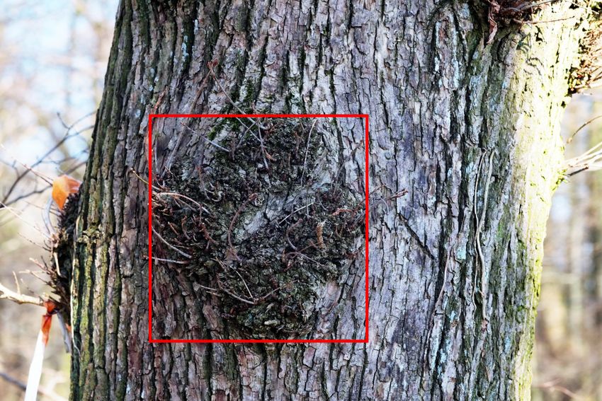
Florian Delconte, Phuc Ngo, Bertrand Kerautret, Isabelle Debled-Rennesson, Van-Tho Nguyen, Thiery Constant
1 Introduction
The development of trees is under the control of genetic factors in interaction with different com-
ponents of their environment. This development results from different meristems producing living
tissues, reacting to the ambient conditions, and producing also new meristems throughout the life of
the tree. Thus, buds, leaves, branches, wood and bark result from such biological processes. This
ability is essential for the tree to cope with the constraints evolving during its whole life, for adapting
its structure as it grows and looks for light. Of course, these constraints are dependent on climatic
conditions and on competition for light, water and nutrients with the tree’s neighbors. They can also
be linked to events such as frost cracking longitudinally the log, or strong wind breaking branches,
or activity of insects or animals, or forester’s action. This ability produces efficient elements for pho-
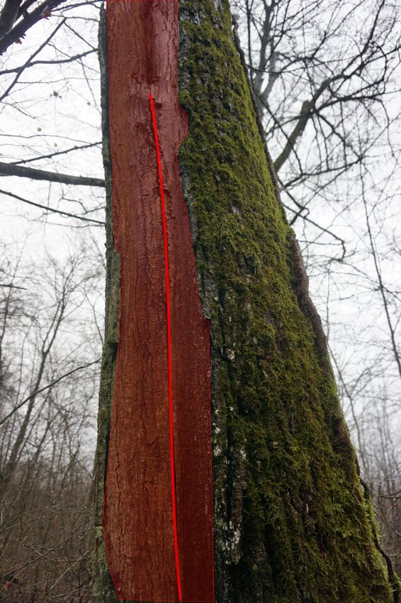
tosynthesis like branches supporting leaves, but also less efficient elements like burls in Figure 1 (a).
It also enables the tree to self-repair when a branch disappears as illustrated in Figure 1 (b,c,d),
or when a frost crack occurs in Figure 1 (f), or when the bark is damaged during the harvesting
of neighbors, as in Figure 1 (e). The result is an alteration of the internal wood structure, which
can be problematic for wood use as a material, but it also coincides with a modification of the bark
structure. The later provides information about the size of the internal singularity and eventually
about its developmental trajectory, especially in case of branches’ scars.
The goal of this work is to automatically detect singularities (or “defects” in industrial context)
located on the log surface. The detection of these singularities is an important step to determine the
commercial value of trees and to optimize the processes that transform them into wood. It is not an
easy task since each type of singularity presents many inter and intra species geometrical variations.
In previous work [1], we proposed a method based on the construction of a relief map combined
with a convolutional neural network (CNN) allowing the accurate segmentation of singularities from
input LiDAR 3D points of tree bark surface. In this paper, the algorithms of the proposed method
are detailed together with the correspondence between algorithms and implementations. An online
demonstration for testing the proposed method is available3 . Moreover, we improve the generation
of the relief map allowing to process input meshes of the partial tree bark surface. Finally, new
experiments are presented in Section 4. A discussion of different parameters influence and limits
for generating the relief map is given in Section 6. Before describing the segmentation method and
algorithms, we first briefly give an overview of the main related works in the following section.
2 Related Works
In general, singularities (or defects) on the surface of a tree bark are distinguishable from the rest
of the trunk because they form a local variation of relief. Singularity detection methods considered
in this paper can be classified into two groups: the classical methods and the deep learning based
methods.
2.1 Classical Methods
In 2013, Kretschmer et al. [8] proposed a semi-automatic method for measuring branch scars on the
surface of tree trunks using terrestrial laser scanning (TLS, also called topographic LiDAR) data.
This method is based on a cylinder fitting along the main axis of the trunk. From this cylinder, a
distance map is generated. This 2D map allows the authors to measure manually the dimensions of
the branch scars on the tree surface. However, due to the non-cylindricity of the trunk, long vertical
traces are observed on the distance map (see Figure 2).
3
https://ipolcore.ipol.im/demo/clientApp/demo.html?id=369
2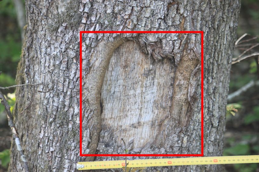
CNN-based Method for Segmenting Tree Bark Surface Singularites

                 (a) Burl (Oak)

            (b) Branch scar (Beech)

         (c) Branch scar (cherry tree)

         (d) Little branch scar (Beech)

           (e) Damaged bark (Oak)
                                                                          (f) Frost crack (Oak)

Figure 1: Examples of tree bark surface singularities (also called defects): branch scar, burl and frost crack. The singularities
are highlighted in red.

                                                               3
Florian Delconte, Phuc Ngo, Bertrand Kerautret, Isabelle Debled-Rennesson, Van-Tho Nguyen, Thiery Constant

                               (a) Cylinder fitting                              (b) Distance map

Figure 2: Singularity detection based on cylinder fitting: (a) the cylinder fitted from the point cloud, with d the distance
used to compute the distance map. (b) Illustration extracted from [8].

    Based on another tree bark surface representation, Nguyen et al. [11] proposed an automatic
singularity segmentation method. This method takes as input a mesh reconstructed from TLS data.
It builds the centerline [5] of the trunk. This centerline allows to compute a local representation of
the relief at each point of the trunk mesh. Then, the automatic thresholding of Rosin [16] is used
to segment the surface singularities. This method will be further detailed in Section 3.1.1. On ten
meshes, the authors obtain an F1 score of 0.71. In 2020, they successfully classified the segmented
regions [10] using a random forest learning process. The singularities regions were classified into four
classes: branch, branch scar, bush, small singularities. The authors obtain an average of 0.86 F1
score on all classes, but only 0.46 on small singularities.

2.2     Deep-learning Based Methods
In a related context of the defect detection on surfaces of cylindrical objects, Tabernik et al. [17]
proposed a method to detect surface defects on cylindrical metal parts. Grayscale intensity images
of the surface are generated. A network of successive convolution layers and max pooling is used
to segment cracks on the surface image. Then, a decision network made of a convolution layer and
a final fully connected layer allows to decide whether or not there is a defect on the surface image.
The proposed strategy is original and appears efficient for the specific case of defects on cylindrical
metal parts. This is however not suitable to the singularities considered in our work.
    The initial method [1] on which this paper relies can also be classified as a deep-learning based
method. In particular, the learning process is performed on images generated from input meshes
using the notion of delta distance [11]. The present strategy aims at improving the accuracy of the
segmented regions. More precisely, the main idea of the method is to build a 2D view of tree bark
surface from TLS data, called a relief map in order to train a CNN to the task of segmenting
regions of particular intensities. The 2D segmentation is then redeployed back in 3D to extract the
points corresponding to the singularity on the input mesh.

3     Singularity Segmentation
This section describes our method which consists of three steps (see Figure 3). Firstly, a 2D map
is built from a 3D mesh of tree bark surface, called relief map (Section 3.1). This process stores
the 3D point indexes in a 2D array, called discretization. In the second step, the singularities are

                                                             4
CNN-based Method for Segmenting Tree Bark Surface Singularites

segmented on the relief map by using a deep learning process allowing to overcome the complexity
of the singularity shapes (Section 3.2). For this, we consider the U-Net architecture [14]. In the last
step, the segmentation is used to recover the 3D points corresponding to the singularities thanks to
the discretization (Section 3.2.2).

                                  Figure 3: Pipeline of the proposed method [1].

3.1     2D Representation of 3D Mesh
3.1.1   Important Concepts from Previous Work
We recall hereafter several concepts that are used in the rest of the article: (i) centerline extraction
method [5, 6], (ii) cylindrical coordinate system, and (iii) local representation of the relief with the
notion of delta distance [11, 12].
    The centerline of a trunk consists of several segments. It is obtained by accumulating along the
normals of the mesh faces in a voxel space and filtering with a confidence vote. As the trunk shape
can be irregular, an optimization process is performed to obtain a smooth centerline (see Figure 4).
    Due to the nature of the points on the trunk surface, we consider an alternative coordinate system,
called cylindrical coordinates, which is simply a combination of the polar coordinates in the xy-plane
with the z coordinate along the centerline. It allows to easily access neighbors of points on the trunk
surface. More precisely, each point in Cartesian coordinate P (x, y, z) is transformed into cylindrical
coordinates (rP , θP , zP ) with a local coordinate system (Ci , ui , vi , wi ) defined for each segment Ci of
the centerline, such that
   • rP is the distance between P and P 0 , the projection of P on the segment Ci of the centerline,
   • zP is the height of P along the centerline by summing the segment lengths of the centerline,
   • θP is the angle between P P 0 and the axis vi of the local coordinate system associated to Ci .
   The delta distance, noted by δP , is a local representation of the tree bark relief. It is computed
on a rectangular area PP around the point P (see Figure 5 (a)). The central straight line fitting the

                                                        5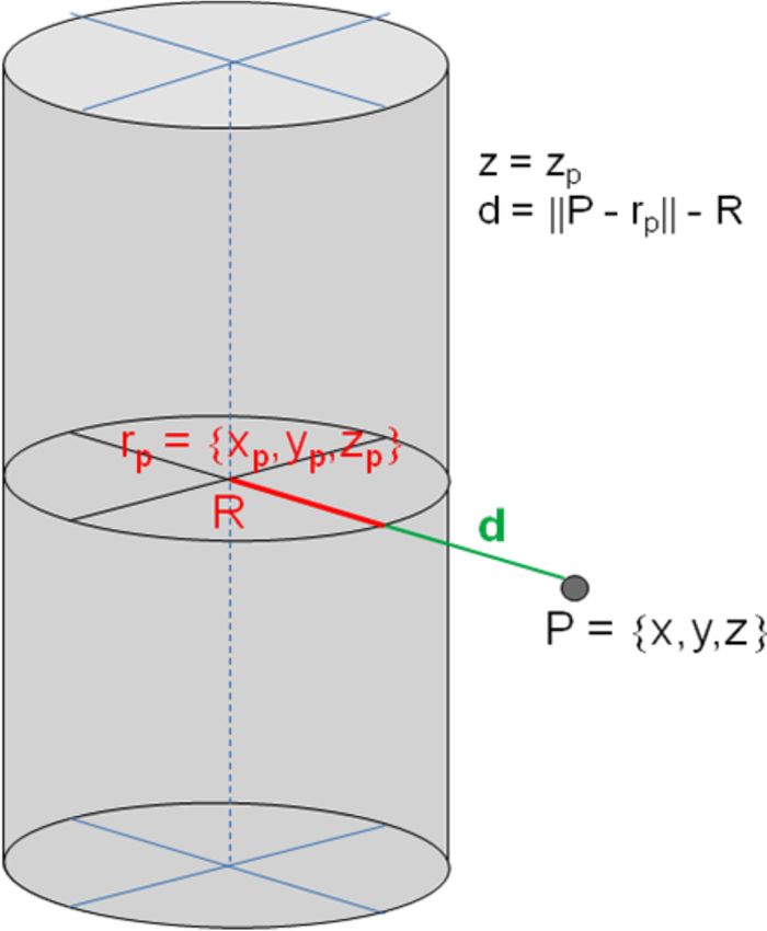
Florian Delconte, Phuc Ngo, Bertrand Kerautret, Isabelle Debled-Rennesson, Van-Tho Nguyen, Thiery Constant

        (a) accumulation process                                          (b) centerline result

Figure 4: Illustration of the main idea of the centerline extraction algorithm: (a) accumulation step from surface faces fk
and fj in the direction of their normal vectors (−
                                                 → and −
                                                 n k
                                                         →); (b) show the resulting centerline on the whole mesh.
                                                         n j

               (a) Rectangular patch PP centered on P                              (b) Delta distance

Figure 5: (a) A patch in blue, associated to the red point P, is used to compute the reference distance of this point. (b)
Computation of δP for the red point. See [11] for more details.

points of PP is calculated by a RANSAC based linear regression. The reference distance of the point
P , noted by r̂P , is the distance from the projection of P on this straight line to the corresponding
segment of the centerline (see Figure 5 (b)). The difference between rP and r̂P represents the relief
of the tree bark at the point P : δP = rP − r̂P . More details of this part can be found in [12].

3.1.2     Discretization

The points in cylindrical coordinates are used to construct a 2D array of height × width cells storing
indexes of the corresponding points. This array is called discretizationMap. By convention, the first
(horizontal) and second (vertical) dimensions are respectively the angle θP and height zP values.
Thus, the discretizationMap’s height is equal to the trunk height. It is computed as the difference
between the z components of the points having the greatest and smallest heights. The discretization-
Map’s width, as proposed in [1], is calculated as the average circumference of the trunk, forcing our
segmentation method to work on complete trunks while the calculation of the centerline can work
on partial trunks (in Figure 7 (a), the centerline is built on a mesh of a partial trunk). In this work,
the discretization is improved by fitting the width of the discretizationMap with highest arc length
of the mesh. To approximate this value, we consider a binary array T initialized to 0. The size of
T is set by the P ad parameter. This array is used to maintain an occupancy map and updated by
going through all mesh points. For each point, its index i on T is computed from its θP angle of the

                                                            6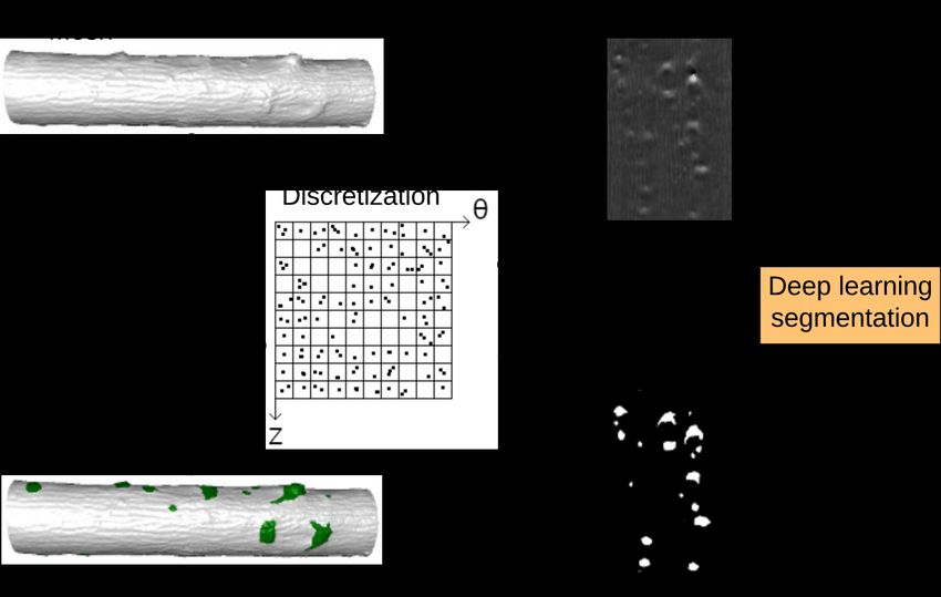
CNN-based Method for Segmenting Tree Bark Surface Singularites
Figure 6: Computation of the partial circumference of the trunk.
cylindrical coordinate
P ad − 1
i = θP ∗ , (1)
2π
where dxc represents the nearest integer to x. The array T is marked at index i of the point with
value 1. Figure 6 shows an illustration of T for P ad = 16 where the mesh points have changed 11
array values from 0 to 1. After all points have been processed, the arc length (discretizationMap’s
width) is computed as follows
(P ad − nbZero)
width = 2π ∗ ∗ meanR , (2)
P ad
where nbZero is the total number of 0 in T , and meanR is the average radii rP of all points belonging
to the trunk mesh. The width value is rounded to the nearest integer.
The discretizationMap has height × width cells. For each point of the mesh, we compute its
position, posX and posY , of the cell in the discretizationMap. The position posX, associated with
θP , has to take into account the first value f1 (the closest angle to 2π or 0) which is associated with
the angular interval computed from the binary array T . The trunk can be partial and therefore the
angle interval can be reduced to [f1 , upperBA − f1 ] with upperBA the angular coverage of the trunk.
The value of upperBA can be approximated using T
(P ad − nbZero)
upperBA = 2π ∗ . (3)
P ad
An angular shift is computed to replace the interval of θP between [0, upperBA]. This shift is ob-
tained by looking for a pattern ‘01’ (framed in blue in Figure 6) in T . The index, f irstIndexN oN ull,
is the index at the position of the cell ‘1’ of the pattern ‘01’. The shift is then given by
f irstIndexN oN ull
shif t = 2π − ∗ 2π . (4)
pad
Finally, posX and posY are given by
width − 1
posX = ∗ ((θP + shif t) mod 2π − upperBA) + width − 1,
upperBA (5)
posY = z − minH.
P
7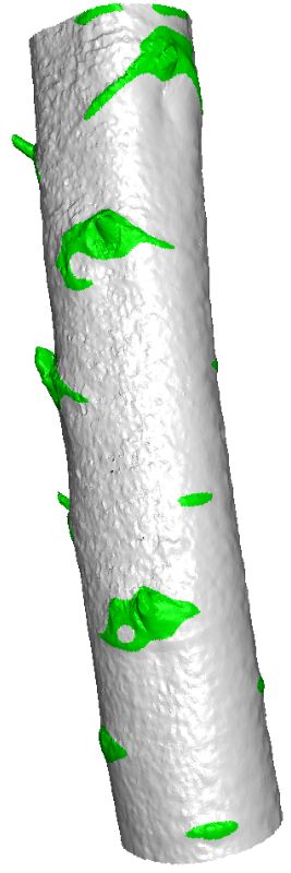
Florian Delconte, Phuc Ngo, Bertrand Kerautret, Isabelle Debled-Rennesson, Van-Tho Nguyen, Thiery Constant

   This step of discretization is described in Algorithm 1. In the code, it corresponds to the function
computeDicretisation of the class UnrolledMap in the package ReliefMap.

 Algorithm 1: 2D discretization of the 3D tree mesh
 → see C++ code: function computeDicretisation of class UnrolledMap in package ReliefMap
   Input: 3D points in cylindrical coordinate system (height, angle, radius): CP oints
   Input: Granularity on angle values to estimate arc length of the log: P ad
   Output: discretizationM ap : a 2D container with the CPoints index distributed in the cells
 1 Let maxH be the maximum height of CP oints
 2 Let minH be the minimum height of CP oints
 3 Let meanR be the means of radius of CP oints
 4 Let T be a binary tabular of size P ad initialized with 0 values
 5 height ← (maxH − minH) + 1                                         // height of the relief map
 6 foreach p ∈ CP oints do
 7    i ← dp.angle ∗ pad/2πc                                                 // round to nearest
 8    T [i] ← 1
 9   f ind ← f alse                                   // boolean value to search ‘01’ pattern in T
10   F irstIndexN otN ull ← 0                         // store the ‘1’ index in ‘01’ pattern found
11   id ← 0                                                       // current index to loop over T
12   while !f ind or id < P ad do
13       currentV alue ← T [id]
14       nextV alue ← T [(id + 1) mod (pad − 1)]
15       if currentV alue = 0 and nextV alue = 1 then
16           f ind ← true
17           F irstIndexN otN ull ← id + 1
18      id ← id + 1
19   Let nbZero the number of zeros in T
20   width ← d2π ∗ (P ad − nbZero/P ad) ∗ meanRe                      // width of the relief map
21   upperBA ← (P ad − nbZero/P ad) ∗ 2π                    // upper bound of angle in CP oints
22   shif t ← 2π − (f irstIndexN oN ull/pad ∗ 2π)                  // shift to apply on CP oints
23   Initialize discretizationM ap to [height, width]
24   for i = 0 to CP oints.size() − 1 do
25       shif tedCurrentAngle ← (CP oints[i].angle+shif t) mod 2π// apply shift and use modulus
25       currentHeight ← CP oints[i].height
26       posX ← (width − 1/upperBA) ∗ (shif tedCurrentAngle − upperBA) + width − 1
27       posY ← currentHeight − minH
28       discretizationM ap[posY ][posX] := i                   // push current index in the cell

3.1.3    Relief Map
From the 2D structure – the discretizationMap – containing for each cell a set of index points, we
will build an image in which the intensity of each pixel is calculated with the corresponding cells in
the discretization. It is called a relief map. In the following, we describe the multi-resolution process
(Algorithm 2) allowing to generate the graylevel relief map with fixed scale from the discretization-
Map.
    The relief map is built through the discretization process. The map domain is rectangular but the
trunk does not necessarily cover the whole area. During the loop over the discretizationMap cells,

                                                     8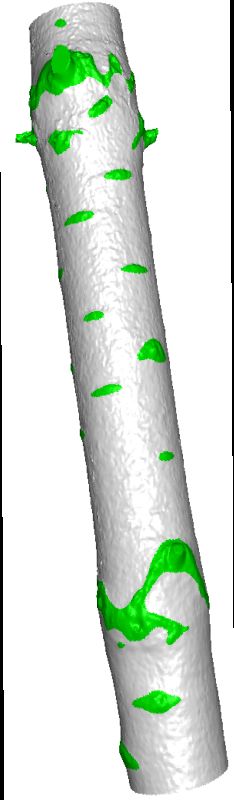
CNN-based Method for Segmenting Tree Bark Surface Singularites

we check if a pixel could be represented by an intensity. This consists in trying to reach the edges
of the discretizationMap, if at least one cell is not empty during the process, then the pixel could be
represented by an intensity. We see in Figure 7 (b), a relief map obtained from a partial trunk, the red
pixels are those whose intensity will not be calculated during the discretization process. Algorithm 3
is used to check if a cell of the discretizationMap could be represented. The function corresponding
to this algorithm is detectCellsIn in the class UnrolledMap of the package ReliefMap.

                            (a)                                                         (b)
         Figure 7: (a) Partial mesh with centerline in green. (b) Partial relief map with outside pixels in red.

     For each cell, a value is chosen according to the delta distance (δP ) of points in the cell. This
distance δP represents the local relief of each point, its calculation is detailed in [11] and reported in
Section 3.1.1. If the current cell is not empty in the discretizationMap, we choose the maximum δP
of all points contained in the cell. Otherwise, a multi-resolution analysis is performed. It consists in
looking for the missing information in cells resulting from the discretizationMap reduced by a factor
 1
2n
   , with n = 1, . . . , M axdF until the cell contains at least one point (M axdF is a parameter of the
multi-resolution search function, it allows to limit the search). More precisely, the points contained
in the larger cells are obtained by accumulating those of the unreduced cells of the discretizationMap
on a square window of width 2n . Finally, we choose the maximum δP of points contained in the
studied cell. Algorithm 5 allows to extract the points in lower resolution and Algorithm 4 gives
the maximum relief representation of a set of points. They correspond respectively to the functions
getIndPointsInLowerResolution and maxReliefRepresentation in the class UnrolledMap of the
package ReliefMap.
     A grayscale image is generated from relief map, by using a single static intensity scale where
intensityP erCm grayscale levels correspond to one centimeter. Associated to this parameter, a
cutoff interval of minimal and maximal heights ([minRV, maxRV ]) is considered to ensure that all
levels can be represented in the usual [0, 255] range. The minimal value minRV is a parameter of
our method and the maximal value maxRV is simply given by
                                                             1
                               maxRV = 255 ∗                         + minRV.                                      (6)
                                                     intensityP erCm
   The resulting grayscale value is deduced as follows

                                         relief V alue − minRV
                             grayscaleV alue =                  ∗ 255.                    (7)
                                           maxRV − minRV
   Algorithm 6 allows to generate the grayscale relief map. It is implemented in the function
toGrayscaleImageFixed, in the UnrolledMap class of the package ReliefMap.

3.2    2D Segmentation
The relief map allows a 2D representation of the trunk. The 3D problem of surface singularity
detection becomes a 2D problem of binary-image-classification in which each pixel of the relief map

                                                           9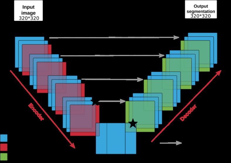
Florian Delconte, Phuc Ngo, Bertrand Kerautret, Isabelle Debled-Rennesson, Van-Tho Nguyen, Thiery Constant

     (a)        (b)         (c)          (d)         (e)         (f)         (g)         (h)          (i)         (j)

     (k)        (l)         (m)          (n)         (o)         (p)         (q)          (r)         (s)         (t)

Figure 8: Examples of relief maps after multi resolution analysis. White color for stronger reliefs. Examples of singular-
ities are highlighted in red frames, one singularity per relief map. Here is the correspondence between relief map and
tree species: (a,b,c,d)=Alder, (e,f,g,h)=Aspen, (i)=Beech, (j,k)=Birch, (i)=Horn beam, (m)=Linden, (n,o)=Red oak,
(p,q)=Wild cherry, (r,s)=Fir, (t)=Elm.

 Algorithm 2: Multi resolution analysis to compute missing information for empty cells
 → see C++ code: computeNormalizedImageMultiScale() of class UnrolledMap in package
 ReliefMap
                                                            1
   Input: Maximum resolution to reach during analysis : 2M axdF
   Output: relief Image : 2D image of the relief
 1 Let height and width be the height and width of discretizationM ap
 2 dF ← 1                                                    // actual decrease resolution factor
   needDisplay ← false
 4 for i = 0 to height − 1 do
 5    for j = 0 to width − 1 do
 6        needDisplay ← detectCellsIn(i,j)                                    // see Algorithm 3
 7        if needDisplay then
 8            relief=maxReliefRepresentation(i,j,0)                          // see Algorithm 4
 9            dF ← 1
10            while relief = −1 and dF < M axdF do
                                                                                               1
11                relief ← maxReliefRepresentation(i,j,dF)// relief of the current cell at 2dF
12                dF ← dF + 1
13               relief Image[i, j] ← relief

                                                           10
CNN-based Method for Segmenting Tree Bark Surface Singularites
Algorithm 3: Verify whether the cell is on the trunk
→ see C++ code: detectCellsIn() of class UnrolledMap in package ReliefMap
Input: Index of the studied cell : (i, j)
Input: 2D Discretization of the 3D points : discretizationM ap
Output: CellsIn : Boolean, true if one cell is considered on the trunk
1 CellsIn ← true
2 iU p ← i
3 IndsCell ← discretizationM ap[i][j]
4 while IndsCell is empty and (iU p > 0) do
5 iU p ← iU p − 1 // Decrement to reach the top
6 IndsCell ← discretizationM ap[iU p][j]
7 Let iDown,jLef t,jRight be the reached index obtained by the same procedure to reach both
left and right respectively
8 if iU p = 0 and IndsCell is empty then
9 same check for iDown, jLef t, jRight
10 CellsIn ← f alse
Algorithm 4: Compute relief representation at one cell in specified resolution
→ see C++ code: maxReliefRepresentation() of class UnrolledMap in package ReliefMap
Input: Index of the studied cell : (i, j)
Input: Decrease resolution factor : dF
Input: Relief representation for each 3D point: relief Representation
Output: maxRelief : relief representation of one cell with a specified resolution
IndexesInCell ← getIndPointsInLowerResolution(i,j,dF) // see Algorithm 5
2 if IndexesInCell is not empty then
3 maxRelief ← search for the maximum relief value in IndexesInCell
else
5 maxRelief ← −1 // conditional value
// Same procedure for to compute the mean or median relief representation
Algorithm 5: Search indexes in discretization map at one cell in lower resolution
→ see C++ code: getIndPointsInLowerResolution() of class UnrolledMap in package
ReliefMap
Input: Index of the studied cell: (i, j)
Input: Decrease resolution factor: dF
Input: 2D Discretization of the 3D points: discretizationM ap
Output: outP utInd : Index of the 3D points in a cell at a lower resolution
dF
1 down_f actor ← 2
2 itopLef tCorner ← (i/down_f actor) ∗ down_f actor
3 jtopLef tCorner ← (j/down_f actor) ∗ down_f actor // round to lowest integer
4 for k = itopLef tCorner to itopLef tCorner + down_f actor do
5 for l = jtopLef tCorner to jtopLef tCorner + down_f actor do
6 if k < height and l < width then
7 outP utInd := discretizationM ap[k][l] // push indexes at pos (k,l)
11Florian Delconte, Phuc Ngo, Bertrand Kerautret, Isabelle Debled-Rennesson, Van-Tho Nguyen, Thiery Constant
Algorithm 6: Convert to grayscale image with fixed scale
→ see C++ code: toGrayscaleImageFixed() of class UnrolledMap in package ReliefMap
Input: Number of intensity to represent 1 cm : intensityP erCm
Input: Minimal relief representation minRV
Input: 2D image of the relief : relief Image
Output: grayScaleRelief Image : Grayscale image of the relief
1 maxRV ← (255 ∗ (1/intensityP erCm)) + minRV // Maximal relief representation
2 Let grayScaleRelief Image get the same size than relief Image
foreach pixels ∈ relief Image do
4 relief V alue = relief Image(point)
5 if relief V alue < minRV then
6 grayscaleV alue ← 0
else if relief V alue > maxRV then
8 grayscaleV alue ← 255
else
10 grayscaleV alue ← ((relief V alue − minRV )/(maxRV − minRV )) ∗ 255
11 grayScaleRelief Image(pixel) ← grayscaleV alue
will be classified as singularity or not. We can see in Figure 8 that singularities on tree barks may have
arbitrary size, shape and orientation. Furthermore, the roughness of the tree bark, the variability of
singularities for the same species and between different species make the detection task difficult to
automate by conventional segmentation algorithms. To overcome this, we opted for a segmentation
by a supervised deep learning approach. In Section 3.2.1, we explain the generation of training pairs
(example/label). Section 3.2.2 details the trained CNN architecture of U-Net [15].
3.2.1 Training Data
The singularities (or defects) have been hand-segmented on the meshes (and verified by experts).
This information allows to associate to each relief map an image labeled in black and white. The
passage of 3D points to 2D labeled image is done by a similar process as described in Section 3.1.
The difference is that, instead of using δP to represent reliefs in gray level, the pixels corresponding
to the singularities have intensity 255 (white) and the others have intensity 0 (black). Besides, as can
be seen in Figure 9 (a), some pixels belonging to the singularities remain black. The multiresolution
process is not used here because it would tend to enlarge the singularities. Instead, a closing and
opening operation with a kernel of size 3 × 3 is applied on the labeled image (see Figure 9 (b)). In
Figure 9 (c) we see the resulting relief map associated to the labeled image.
The size of the relief map (and the labeled images) is different from one mesh to another because
the circumference and height of the trunk are not always the same. To increase the number of
training data, we have extracted patches of size 320 × 320 pixels following two strategies:
1) with singularities: the process consists in finding the barycenters of connected components in
the labeled images. For each barycenter, we extract a centered patch of size 320 × 320 pixels
in both labeled image (as ground-truth) and relief map. If a singularity is too close to the edge
of the image, a translation is performed so that the patch still contains the singularity and is
included in the image (see Figure 10).
2) without singularities: the process consists in finding rectangular areas of size 320 × 320 pixels
containing no white pixels in the labeled image. When such an area is found, the patch is
12CNN-based Method for Segmenting Tree Bark Surface Singularites
(a) (b) (c)
Figure 9: labeled image and corresponding relief map with zoom in rectangular area: (a) before closing and opening
operation, (b) after closing and opening operation and (c) corresponding relief map.
(a) Extracted patches with singularities from relief maps
(b) Extracted patches with singularities from annotated maps
Figure 10: Some samples from training data.
extracted in the relief map and a black image is generated as ground-truth.
Following this splitting process, different techniques were also applied on the resulting patches to
enlarge further the data. In particular, we consider the following operations: rotation in range 0◦ to
20◦ , flipping vertically and horizontally, zooming of ±30% and randomly deleting a rectangular area
[2] with a 0.5 probability. Note that this data augmentation is performed on the fly, i.e., during the
training process.
3.2.2 U-Net Architecture for Segmentation
U-Net is a fully convolutional network. It is widely used in bio-medical image segmentation [3, 19, 20].
More recently, U-net has been applied in other fields such as satellite image segmentation [4, 18] or
tunnel object detection [13]. This architecture is well-known for its performance when trained with
very few images.
In general, a U-net network consists of two parts: encoding and decoding. The encoding part looks
like a classical convolutional network architecture. It consists in applying successively convolutions
13Florian Delconte, Phuc Ngo, Bertrand Kerautret, Isabelle Debled-Rennesson, Van-Tho Nguyen, Thiery Constant
and max pooling operations. The decoding part is made of up-sampling operations followed by a
concatenation with the layer of the same level in the encoding part.
For our problem of detecting tree bark surface singularities, we made several changes to the
original U-Net. In order to reduce the over-fitting of the considered neural network, we apply a
regularization technique, called drop-out. More precisely, two dropout layers are added, with a 0.5
probability, to randomly drop some of the connections between layers. At the first level, there are 32
filters per convolution layer. Then the number of filters is doubled at each level. Besides, due to the
dying ReLU problem [9] the Leaky ReLu activation function is employed instead of ReLU from the
original architecture. Finally, in the last layer, we use a sigmoid activation function instead of the
soft-max function to ensure the output pixel values range between 0 and 1. The proposed network
architecture is illustrated in Figure 11.
Figure 11: The architecture for tree bark singularities detection based on U-Net [15].
Once trained, the network’s prediction produces an image whose pixel intensity corresponds to a
probability score of belonging to a singularity pixel. The higher the grey level, the more the pixel is
considered as a singularity by the network and vice versa. We can see in Figure 12 two examples of
output of the trained network.
From the prediction result, a threshold is applied to retrieve a 2D segmented image in black and
white. The white pixels correspond to the regions of the relief map considered as singularities. In
order to obtain the singularities on 3D mesh from white pixels of the segmentation results, an inverse
discretization is performed. More precisely, the discretization has the same size as the segmentation.
The indices of the points contained in the cells of the discretization at the position of the white pixels
are extracted. They correspond to the singularities in 3D. In Figure 12, we can see two examples of
extracted points in green color from the segmented results.
14CNN-based Method for Segmenting Tree Bark Surface Singularites
input output binary output (t=0.5) mesh
Figure 12: Examples of output of our U-net [15] inspired architecture.
4 Experiments
4.1 Dataset
To test our method we have 25 trunk meshes: 10 from [11] and 15 new data manually annotated.
This database contains 11 tree species: beech, birch, elm, fir, red oak, wild cherry, aspen, horn beam,
lime, and alder. The studied trunks have between 366 and 896 cm of circumference and between
694 and 1150 cm of height. The visible surface singularities are mainly branch scars and burls, there
are also some small singularities whose type is not distinguishable. In Figure 13, we can see some
examples of 3D point clouds from the dataset. We randomly pick 5 trunks among the 25 to test the
method and kept the others for training.
Beech Birch Red oak Aspen Charme Linden Alder
Figure 13: Examples of trunks (logs) of different tree species, captured from LiDAR point cloud including reflectance values.
15Florian Delconte, Phuc Ngo, Bertrand Kerautret, Isabelle Debled-Rennesson, Van-Tho Nguyen, Thiery Constant
4.2 Cross-validation Studies
The cross-validation consists in training k models by varying the data used for training and validation
in such way that the model is validated on k different folds. In our experiment k = 5. The relief maps,
generated from the training data, are split into patches of 320×320 pixels (see Section 3.2). After the
splitting process, we obtain 456 patches. Five models are trained on groups of patches with a ratio of
1
5
for the validation and the rest for the training. These groups of patches are constructed so that the
validation data is different for each model. Once the network is trained, we apply the segmentation
method (see Section 3) on the 5 test trunks, and obtain a set of points classified as singularities.
They are then compared to the ground-truth. It should be mentioned that, in [1], we performed a
cross validation on the same data. However, the experiment was different, we wanted to test our
method on all the available data. Here, the cross validation allows us to test the performances of
the segmentation model and its sensibility to the learning data. Figure 14 summarizes the difference
between the two cross validation procedures on a base of ten examples.
The training process was performed on a GPU (NVIDIA Geforce RTX 2080Ti with 12Go RAM).
We used the Adam optimiser [7] with the two parameters β1 = 0.9 and β2 = 0.99 (default values in
tensorflow), and set the learning rate at 0.0001. We trained our network for 40 epochs, each epoch
comprised 111 steps with 10 images per batch. As for the parameters dropout rate δ and Leaky
ReLu activation α, several values have been tested, and we come out with δ = 0.5 and α = 0.01 for
the smallest loss function (binary cross entropy) on the validation set. It should be mentioned that
our training is quite fast, it takes about 14 seconds per epoch.
Figure 14: Difference between the cross validation in [1] (left) and our cross validation (right).
4.3 Results
The results are presented in Table 1. For evaluating the method, 3 metrics are used: precision, recall
and F1 score. Each row contains the results of the training model on the test data. The average
and standard variation are calculated over the 5 models. Figure 15 shows the segmentation results
of our method (using K4 as model segmentation) with a comparison to the ground-truth. On the
examples WildCherry1, Redoak1 and Fir1, we obtain an average F1 score > 0.815. The F1 score
is lower on Aspen2 and Alder2. For Aspen2, we notice a decrease of the recall value compared to
the other examples. The regions segmented by our method correspond well to singularities, however
the ground-truth covers wider zones of defects. This results in an increase of the false negative
rate and a decrease of the recall value. For Alder2, it is the precision value that is lower. Around
the branch scars, the trunk forms cavities. Our segmentation method tends to encompass these
16CNN-based Method for Segmenting Tree Bark Surface Singularites
structures which increases the false positive rate and therefore the accuracy decreases. Despite this
difference in performance, the low values of standard variation show that the 5 models provide close
performance measures even for Aspen2 and Alder2. This makes us believe that the training is robust
to the considered dataset.
WildCherry1 Redoak1 Fir1 Aspen2 Alder2
K-Folds
prec recall F1 prec recall F1 prec recall F1 prec recall F1 prec recall F1
K0 0.825 0.88 0.851 0.893 0.886 0.889 0.831 0.815 0.822 0.877 0.561 0.682 0.594 0.878 0.707
K1 0.837 0.829 0.831 0.867 0.861 0.863 0.867 0.731 0.79 0.816 0.545 0.652 0.567 0.799 0.663
K2 0.831 0.868 0.848 0.878 0.877 0.877 0.857 0.778 0.814 0.894 0.611 0.725 0.593 0.831 0.691
K3 0.846 0.862 0.853 0.853 0.889 0.87 0.854 0.802 0.826 0.849 0.609 0.709 0.6 0.86 0.706
K4 0.811 0.911 0.857 0.871 0.906 0.888 0.827 0.82 0.823 0.88 0.636 0.737 0.596 0.885 0.711
Mean 0.83 0.87 0.848 0.872 0.884 0.877 0.847 0.789 0.815 0.863 0.592 0.701 0.59 0.851 0.696
Std 0.013 0.03 0.01 0.015 0.016 0.011 0.017 0.036 0.014 0.031 0.038 0.034 0.013 0.036 0.020
Table 1: Cross validation results for the considered 5 folds.
WildCherry1 Redoak1 Fir1 Aspen2 Alder2
Figure 15: Colorized mesh to show the difference between the ground-truth and segmentation obtained with the proposed
method. Yellow is true positive, red is false negative and green is false positive.
5 Code
The code is written in C++ and python. The C++ part allows the interaction between mesh
and relief map. The python part allows to use the segmentation model. In addition, the user can
reproduce the results in Table 1.
5.1 Materials
The archive examples_IPOL.tar.gz contains the tree meshes and the ground-truth data files. They
are in two directories: INRAE1a, INRAE1b. The data come from the same acquisition device and have
17Florian Delconte, Phuc Ngo, Bertrand Kerautret, Isabelle Debled-Rennesson, Van-Tho Nguyen, Thiery Constant
been transformed into a 3D mesh using the process described in [10]. Each tree trunk is associ-
ated to three files: the mesh (with extension .off), the point indices corresponding to singularities
(suffixed by -groundtruth-points.id), the face indices corresponding to singularities (suffixed by
-groundtruth.id). The experiments in Section 4 use the files suffixed by-groundtruth.id for eval-
uating the performance of our method. The scaledMeshes directory contains scaled meshes used in
Section 6.4.
The archive model_IPOL.tar.gz contains the models to reproduce the results. They are suffixed
by K following a number between 0 and 4. Images in Section 4 are generated from the model k4.hdf5.
5.2 Dependencies
For compilation of the C++ sources these libraries must be installed:
• DGtal 1_1_0 or later: https://github.com/DGtal-team/DGtal
• GNU GSL: https://www.gnu.org/software/gsl/
• PCL: https://pointclouds.org/downloads/
To use our trained model for the segmentation of singularities on the relief map these libraries
need to be installed (we recommend the user to use a virtual environnement as described in the
tensorflow guide):
• Tensorflow 2.2: https://www.tensorflow.org/install/pip
• tensorflow-addons: https://www.tensorflow.org/addons/overview
• OpenCv: https://pypi.org/project/opencv-python/
5.3 Generate the Relief Map (C++)
Once the dependencies are installed and the sources downloaded, the project is built with the fol-
lowing commands:
cd TLDDC
mkdir build
cd build
cmake .. -DDGtal_DIR=/path/to/DGtalSourceBuild
make
Three executable files are generated in the build directory: segunroll , groundtruth, segToMesh.
segunroll allows the user to build the grayscale relief map. The image format is pgm. Three
files are generated: reliefmap_info, cylPoint, discretize. The file reliefmap_info contains
data relative to the construction of the relief map: height, width, upper bound of the angle of the
mesh points (see Section 3.1.2). All the points of the mesh converted into cylindrical coordinates
are stored in cylPoint using one point per line with: radius, angle and height. The file discretize
contains height × width lines. Each line contains the list of indices of points belonging to the cell of
the discretization (-1 if none). We save this information to avoid having to recalculate it later. The
user can use the following command to generate the relief map:
./segunroll -i InputMesh [-h] [CenterlineParameters] [ReliefMapParameters] -o outputName
• InputMesh: path to a trunk mesh.
18CNN-based Method for Segmenting Tree Bark Surface Singularites
• -h: option for the command line helper.
• CenterlineParameters: chosen according the recommended values in [10].
• ReliefMapParameters: parameters for relief map (--MaxdF, --minRV, --intensityPerCm,
--pad ). They are also set with default values.
• -o: prefix of the output.
For example, you can use this command to reproduce the same relief map used in our experiments:
./segunroll -i INRAE1a/WildCherry2.off -o WC2 –MaxdF 4 –minRV -5 –intensityPerCm 10 –pad 200
groundtruth allows the user to generate a pgm image of the same size as the relief map in black
and white with white for the position of defects on the map. For this, the information previously
calculated and stored in reliefmap_info and cylPoint is used. These labeled images are used to
train our segmentation model, the user can generate them by using the following command (after
generating the files reliefmap_info and cylPoint):
./groundtruth -i InputGrouthTruth -o outputName
• InputGrouthTruth: path to ground-truth, suffixed by: -groundtruth.id
• -o: prefix the output.
For example, you can use this command to reproduce the ground-truth image used in our experi-
ments:
./segunroll -i INRAE1a/WildCherry2-groundtruth.id -o WC_GT
segToMesh allows to extract the 3D points from the output of the segmentation model. The
file discretize allows to make the correspondence between the white pixels (for singularities) and
the 3D points of the mesh (see Section 3.2.2). Two files are generated. A file suffixed by -defect.id
contains the indices of points considered as singularities. A file suffixed by defect.off contains
the trunk mesh with the singularities colored in green. The command to do this operation is the
following (after generating the singularity segmentation by an already trained model):
./segToMesh -i InputMesh -s segmentationMapName -o outputName
• InputMesh: path to the same mesh used to generate the reliefmap.
• -s: path to the segmentation file.
• -o: prefix the output.
The interaction between these different executables is summarized in Figure 16.
To generate the relief map and labeled images of a whole directory at once, you can use the script
makeAllPair.sh (in the run directory) with the following command. The relief map will have the
same name as the mesh and the labeled image will be fixed by _GT.
./makeAllPair.sh PathToMeshDirectory OutputPath
• PathToMeshDirectory: path to the input directory containing meshes.
• OutputPath: path to output directory in which all samples will be moved.
19Florian Delconte, Phuc Ngo, Bertrand Kerautret, Isabelle Debled-Rennesson, Van-Tho Nguyen, Thiery Constant
Figure 16: Interaction between the different executables of the project.
5.4 Extract Patches from ReliefMap and Ground-truth Image (python)
In the run directory, there is a script named train-valid_cut.py . From a relief map and a ground-
truth image, it allows to extract training patches (see Section 3.2.1) and distribute them in the train
and valid directories. From the created patches 80% are distributed in the train directory, and 20%
in the valid directory. These directories must be created before calling the script and both of them
must contain a directory named input and another named output. Here is the command to run:
python3 train-valid_cut.py -i PathToReliefMap -g PathToGT -o outputDir
• PathToReliefMap: path to input relief map.
• PathToGT : path to input ground-truth image.
• outputDir : output directory that must contain two directories named train and valid, which
must contain two directories named input and output.
To perform the patches extraction on all pairs of training images in a directory (generated by the
script makeAllPair.sh) you can use the script named train-valid_cut_All.sh. Here is the
command to run:
./train-valid_cut_All.sh PathToInputDir PathToOutputDir
• PathToInputDir : path to input directory that contains relief map and corresponding ground-
truth image suffixed by _GT.
• PathToOutputDir : output directory that must contain two directories named train and valid,
which must contain two directories named input and output.
5.5 Use our Trained Network (python)
In the run directory, there is a script named predict.py that allows to use the network to segment the
singularities on a relief map. It takes as input an already trained model and a relief map (previously
generated) in pgm format. Two images suffixed by SEG.pgm and SEGTRESH.pgm are generated. The
first one is in grayscale, the second one is in black and white (see Section 3.2.2). Here is the command
to run:
20CNN-based Method for Segmenting Tree Bark Surface Singularites
python3 predict.py InputReliefMap PathToModel Threshold
• InputReliefMap: path to the relief map.
• PathToModel : path to the model.
• Threshold : threshold ([0; 255]) to apply on the network prediction.
5.6 Train a Network with ReliefMap Samples (mix)
Relief map and ground-truth images must be generated by the script makeAllPair.sh. Here is
an example of how to generate these images from the INRAE1b directory and move them to the db
directory:
./makeAllPair.sh examples/INRAE1b/ db/
The learning process requires data to be organized in a directory named train and another valid.
In both of them, there must be a directory named input and another named output. Create them
in a directory named db. The network is trained on patches of size 320 × 320 (see Section 3.2.1), use
train-valid_cut_All.sh to extract these patches:
./train-valid_cut_All.sh db/ db/
Once data is prepared, train the network with the script named train.py . Here is the command:
python3 train.py -i db/ -o prefix
• db/ : database directory that contain train and valid sample.
• prefix : name of the model.
5.7 Test the Complete Process of our Segmentation Method (mix)
In the run directory, there is a script named deep-segmentation.sh. This script allows to call in
succession: segunroll , predict.py , segToMesh. Here is the command to execute it:
./deep-segmentation.sh PathToModel PathToMesh
• PathToModel : path to the model.
• PathToMesh: path to the mesh.
5.8 Reproduce the Results (mix)
In the run directory, there is a script named testK_folds.sh. This script allows to reproduce the
results in Table 1. The segmentation method is tested on 5 examples and 5 models. The name of
the tested mesh is written in the file testKFold_Path.txt at the root of the code repository. The
scripts segunroll , predict.py , segToMesh are called to extract the singularity points of the mesh.
The metrics (precision, recall, F1) are displayed, for each fold, in the terminal. Here is the command
to execute it:
21Florian Delconte, Phuc Ngo, Bertrand Kerautret, Isabelle Debled-Rennesson, Van-Tho Nguyen, Thiery Constant
./testK_folds.sh PathToMeshDirectory PathToModeleDirectory
• PathToMeshDirectory: path to the root of downloaded mesh directory.
• PathToModeleDirectory: path to the root of model directory.
6 Influence of Parameters and Limits
The relief map is the main tool of our method. It greatly influences the quality of the singularity
segmentation. To generate a relief map, there are 4 important parameters. In the following, we
describe the role and the default values of these parameters.
6.1 Depth Parameter in Multi-resolution Analysis: MaxdF
A multi-resolution analysis is performed on the relief map. The purpose of this analysis is to complete
the relief map with information at lower resolution (see Section 3.1.3). During this operation, the
dimensions of the relief map are reduced by a factor of 21n with n ∈ [0, . . . , M axdF ]. In Figure 17,
we can see 5 relief maps coming from the same mesh at different resolutions which decrease by a
factor of two. At the resolution 1, we can see “holes” (pixels with no value) on the relief map,
this missing information will be completed by analyzing the relief map at a smaller resolution. By
reducing the resolution of the relief map, the information it contains is reduced as well (the relief is
less well represented). We stop the multi-resolution search, when the resolution becomes too small.
The M axdF parameter allows us to stop this search. If n = M axdF , the multi-resolution process
is stopped at the first level. In our data, the smallest resolution reached by the multi-resolution
analysis is 214 . Therefore, we set M axdF = 4 as the default value.
1 1 1 1 1
20 21 22 23 24
1
Figure 17: Same relief map with resolution decreasing by 2n factor with n ∈ [0, . . . , 4].
22CNN-based Method for Segmenting Tree Bark Surface Singularites
6.2 Grayscale Parameters: intensity_per_cm and minRV
The singularities are distinguishable from the rest of the trunk because they form a relief variation
on the surface. This variation can be negative or positive. To represent the surface relief variation,
we consider a grayscale relief map. This conversion is done by two parameters: intensity_per_cm
and minRV . The parameter minRV corresponds to the intensity 0 of the relief map for the smallest
relief to represent. It is recommended to use a negative value for minRV , this allows to represent the
whole surface of the trunk. The parameter intensity_per_cm allows to define the number of gray
levels to represent 1 cm of relief. The choice of the value of intensity_per_cm should not be too
high because it determines the maximum representable relief. If intensity_per_cm = 50, the relief
map will be able to represent at most a relief about 5 cm. The value must not be chosen too low
either because some singularities have a very low relief, for example the singularity named “picots”
are not more than 1cm high. By default, intensity_per_cm = 10 and minRV = −5 for all the
relief maps generated for the training or for the tests of the segmentation method.
6.3 Angular Division Parameter: Pad
The width of the relief map corresponds to the maximum arc length of the mesh. To estimate it, we
use an array of size P ad (see Section 3.1.2). The smaller the P ad, the more error will be made on
the circumference of the trunk. For our data, we set P ad = 200 by default.
6.4 Scale Influence
It should be mentioned that the trunks in our database present comparable scale size, with hand-
annotated singularities (see Section 4.1). In order to evaluate the robustness of our method with
respect to the mesh scale, we have changed the scale of the WildCherry1 mesh using the following
values: 0.8, 1.2, 1.5, 3, 5. This experiment is done for the purpose of verifying whether our method
is able to perform the singularity segmentation on larger trunks. Figure 18 shows the relief maps
generated from the enlarged mesh and the associated segmentation. The relief map seems to be
impacted by the scale factor. The perturbation of the relief map by the scale change impacts the
quality of the segmentation. We think that this is due to the fixed size of the rectangular patch used
to calculate the delta distance (see Section 3.1.1). Therefore, it would be necessary to automatically
adapt the rectangular patch size with respect to the studied trunk. Moreover, the relief maps used
to train our models are generated from trunk meshes of similar size. It would be interesting to study
and apply a scale variation on the training data to allow the network to generalize the segmentation
on larger trunks. However, scale changes by a factor of 5 can be considered as very special cases
which are infrequent for usual application cases.
7 Conclusion
In this article, we proposed a method allowing to automatically segment the singularities on the
tree bark surface. It is adapted from [1]. More precisely, the method is based on the construction
of a relief map able to locally adapt itself to the global shape of the trunk, and combines with a
convolutional neural network to improve the resulting segmentation quality. Furthermore, we bring
an improvement in generating relief maps compared to [1]. This improvement allows to build relief
maps from partial meshes of trunks where a cylindrical sector may be missing. Moreover, we detail
the algorithms and the code used to generate the relief map. The cross validation shows that the
training is robust to our database (the standard deviation is low). However, we believe that our
segmentation method would benefit from using more 3D information.
23Florian Delconte, Phuc Ngo, Bertrand Kerautret, Isabelle Debled-Rennesson, Van-Tho Nguyen, Thiery Constant
s=0.8 s=1.2 s=1.5 s=3 s=5
relief map
model prediction
model prediction (t=0.5)
Figure 18: Our method segmentation on the example WildCherry1 at different scales.
In the future, we would like to work on the generation of a new type of map from the trunk
meshes, in particular using the normals from face meshes. It will allow to represent the orientation
of the face meshes in the image. We then will train a CNN to accumulate orientation and relief
information to produce a segmentation. In addition, we plan to address the related objective of
classifying the singularities according to their different types. Such features are interesting to get a
finer estimation of the wood quality.
24CNN-based Method for Segmenting Tree Bark Surface Singularites
Acknowledgment
This research was made possible with the support from the French National Research Agency, in the
framework of the project WoodSeer, ANR-19-CE10-011.
Image Credits
images from the authors.
References
[1] F. Delconte, P. Ngo, I. Debled-Rennesson, B. Kerautret, V-T. Nguyen, and
T. Constant, Tree Defect Segmentation using Geometric Features and CNN, in Re-
producible Research on Pattern Recognition (RRPR), 2021. https://doi.org/10.1007/
978-3-030-76423-4_6.
[2] T. Devries and G.W. Taylor, Improved regularization of convolutional neural networks with
cutout, ArXiv preprint, abs/1708.04552 (2017). https://arxiv.org/abs/1708.04552.
[3] N. Ibtehaz and M.S. Rahman, MultiResUNet: Rethinking the U-Net architecture for mul-
timodal biomedical image segmentation, Neural Networks, 121 (2020), pp. 74–87. https:
//doi.org/10.1016/j.neunet.2019.08.025.
[4] V. Iglovikov and A. Shvets, Ternausnet: U-net with VGG11 encoder pre-trained on ima-
genet for image segmentation, arXiv preprint, (2018). https://arxiv.org/abs/1801.05746.
[5] B. Kerautret, A. Krähenbühl, I. Debled-Rennesson, and J. O. Lachaud, Centerline
detection on partial mesh scans by confidence vote in accumulation map, in International Con-
ference on Pattern Recognition (ICPR), 2016, pp. 1376–1381. http://dx.doi.org/10.1109/
ICPR.2016.7899829.
[6] , On the Implementation of Centerline Extraction based on Confidence Vote in Accumulation
Map, in International Workshop on Reproducible Research in Pattern Recognition, B. Kerautret,
M. Colom, and P. Monasse, eds., vol. 10214, Springer, 2016, pp. 109–123. http://dx.doi.org/
10.1007/978-3-319-56414-2_9.
[7] D.P. Kingma and J. Ba, Adam: A Method for Stochastic Optimization, in International
Conference on Learning Representations, 2014.
[8] U. Kretschmer, N. Kirchner, C. Morhart, and H. Spiecker, A new approach to
assessing tree stem quality characteristics using terrestrial laser scans, Silva Fennica, 47 (2013),
p. 1071. http://dx.doi.org/10.14214/sf.1071.
[9] L. Lu, Y. Shin, Y. Su, and G. Em Karniadakis, Dying ReLU and Initialization: Theory
and Numerical Examples, Communications in Computational Physics, 28 (2020), pp. 1671–1706.
https://doi.org/10.4208/cicp.OA-2020-0165.
[10] V-T. Nguyen, T. Constant, B. Kerautret, I. Debled-Rennesson, and F. Colin,
A machine-learning approach for classifying defects on tree trunks using terrestrial LiDAR,
25You can also read