Vision-based Large-scale 3D Semantic Mapping for Autonomous Driving Applications - arXiv
←
→
Page content transcription
If your browser does not render page correctly, please read the page content below
Vision-based Large-scale 3D Semantic Mapping for Autonomous
Driving Applications
Qing Cheng1 Niclas Zeller1,3 Daniel Cremers1,2
qing@artisense.ai niclas.zeller@h-ka.de cremers@tum.de
Abstract— In this paper, we present a complete pipeline for
3D semantic mapping solely based on a stereo camera system.
The pipeline comprises a direct sparse visual odometry front-
arXiv:2203.01087v1 [cs.CV] 2 Mar 2022
end as well as a back-end for global optimization including
GNSS integration, and semantic 3D point cloud labeling. We
propose a simple but effective temporal voting scheme which
improves the quality and consistency of the 3D point labels.
Qualitative and quantitative evaluations of our pipeline are
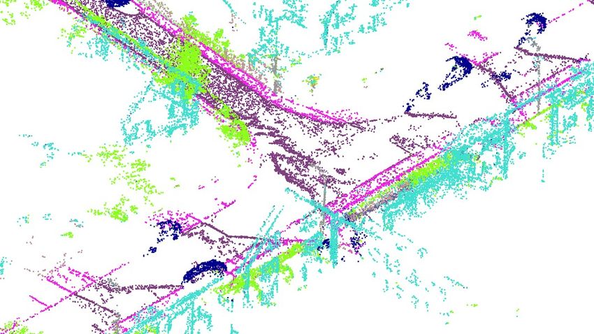
performed on the KITTI-360 dataset. The results show the ef- Fig. 1: Large-scale semantic map of Berlin. Left: We generated a large-
fectiveness of our proposed voting scheme and the capability of scale semantic map covering 8000 km of roads in Berlin with a fleet of
our pipeline for efficient large-scale 3D semantic mapping. The vehicles. Right: Zoomed-in sections of the semantic map show the fine-
large-scale mapping capabilities of our pipeline is furthermore grained 3D reconstruction details of the map.
demonstrated by presenting a very large-scale semantic map
covering 8000 km of roads generated from data collected by a
fleet of vehicles.
Index Terms— 3D mapping, autonomous driving, semantic We believe that the proposed pipeline reveals the potential
segmentation, visual SLAM. of purely vision-based mapping systems for autonomous
driving applications and can be extended towards extracting
I. I NTRODUCTION information like lane markings, etc., although it does not
provide fully vectorized HD maps yet. In Figure 1, we
Autonomous Driving (AD) is among the major technical
demonstrate that our method can be used to create city-scale
challenges pursued by automotive companies and academics
maps based on a fleet of vehicles.
around the globe. One of the most considerable obstacles on
the way to full autonomy is the challenge of 3D perception: Our Contributions in detail are the following:
understanding the 3D world around the vehicle with its vari- • A fully automatic vision-based 3D mapping pipeline
ous sensors. An autonomous vehicle (AV) can perform online that can create large-scale 3D semantic maps efficiently.
path planning and make reliable, safety-critical decisions • A simple but effective temporally consistent point label-
based on such an established environmental model. ing scheme that improves the accuracy of the 3D point
While in the past reliable perception was enabled by equip- labels by taking the structural information provided by
ping a vehicle with all different kinds of sensor modalities, the visual odometry front-end into account.
today’s trends go more towards the use of fewer and cheaper • A benchmark for vision-based 3D semantic mapping
sensors to perceive the surrounding of a vehicle. pipelines, which fuses 3D LiDAR and 2D image ground
State of today, in addition to online perception, environ- truth labels.
mental models are complemented by topological information
of static road furniture. High-definition maps (HD maps)
II. R ELATED W ORK
can provide such redundant and abundant information to
back up the online sensor data. Nevertheless, it is crucial In this paper, we are presenting a pure vision-based se-
to keep such maps up to date due to rapid changes in road mantic mapping pipeline. Therefore, there are basically two
infrastructures, especially in urban environments. Hence, different research streams to which our method relates. One
instead of expensive mapping sensors and manual labeling is visual SLAM, which allows building large-scale 3D maps
processes, lightweight and scalable online mapping pipelines only from image data. The other is semantic segmentation,
become more preferred. which aims to extract semantic information from the captured
In this paper, we are proposing a complete vision-based sensor data. Hence, in the sequel, we review both the state of
pipeline towards the goal of creating scalable and up-to-date the art in visual SLAM as well as in 2D (image-based) and
maps. Our pipeline generates 3D semantic maps at scale 3D (LiDAR-based) semantic segmentation. Furthermore, we
from only a stereo-vision system, as shown in Figure 2. discuss related mapping pipelines based on different sensor
1 modalities. For all these tasks, there exists several popular
Artisense GmbH
2 Technical University of Munich datasets relevant for training and benchmarking [2], [3], [1],
3 Karlsruhe University of Applied Sciences [4], [5], [6], [7].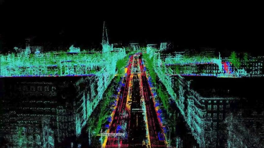
image pixel or 3D LiDAR point). In recent years, research
                                                                                  in this field is heavily driven by large-scale datasets [3], [1],
                                                                                  [4], [5], [6]. Two main work streams are present for semantic
                                                                                  segmentation in robotic and autonomous driving use-cases:
                                                                                  2D semantic segmentation on RGB or intensity images and
                                                                                  3D semantic segmentation on structural 3D representation,
                                                                                  e.g. LiDAR point clouds.
                                                                                     Due to the high resolution of images and the rich tex-
                                                                                  tural information, image-based approaches provide high-
                                                                                  quality segmentation results [25], [26], [27]. In general,
                                                                                  these methods are highly efficient using 2D CNNs. The
                                                                                  pioneering work [25] tackles the semantic segmentation task
                                                                                  with a fully convolutional neural network (FCNN) which
Fig. 2: 3D semantic map generated by the proposed pipeline for sequence 0
of the KITTI-360 dataset [1]. Left: Sparse point cloud generated from direct      can generate a full-resolution semantic mask for an input
visual odometry (VO). Center: Semantic 3D point cloud. Right: Extracted           image of arbitrary size. To utilize more high-level context,
street-level information, including roads, sidewalks, traffic signs/lights. Due   [28], [29], [30], [31] integrate the probabilistic graphical
to the high accuracy and quality, the generated semantic map can be used
to perform further vectorization towards HD map generation.                       models, e.g. Conditional Random Fields (CRFs), into their
                                                                                  network architectures. Another direction is to exploit multi-
                                                                                  scale inputs [32], [33], [34], [35] or spatial pyramid pooling
   1) Visual SLAM: or structure-from-motion (SfM) algo-                           [36], [27], [37], [38] in order to generate feature maps
rithms are at the core of any mapping pipeline. These                             encoding contextual information from different resolutions
methods can be mainly divided into indirect (or keypoint-                         for the final pixel-level classification. The popular encoder-
based) and direct approaches.                                                     decoder architectures learn dense semantic features from
   Indirect approaches extract a set of interest points from the                  the encoded low-resolution feature responses from single or
image and then perform pose and 3D point estimation by for-                       multiple encoder layers and demonstrate promising perfor-
mulating a geometric energy term using the extracted interest                     mance on semantic segmentation tasks with this scale context
points [8], [9], [10], [11], [12], [13]. Here correspondences                     [39], [40], [41], [42], [43], [44]. Attention mechanisms
of interest points between consecutive images are either                          are also introduced to semantic segmentation architectures
established by matching descriptors [8], [9] or based on                          which outshine max and average pooling with the selective
optical flow estimation [12]. While indirect methods gener-                       aggregation of various contextual features [33], [45], [46],
ally provide high tracking robustness, the 3D reconstruction                      [47], [48], [49]. Auto-labelling techniques [50], [51], [48]
is limited to the sparse set of interest points, making it                        and domain adaptation methods [52], [53] are also proposed
insufficient for 3D mapping purposes. This can be overcome                        to alleviate the reliance on the expensive pixel-wisely labeled
by combining an indirect pose estimation with multiple-view                       training data. In our work, we make use of the work proposed
stereo (MVS) [14], [15], [16].                                                    by [50], which demonstrates state-of-the-art performance in
   Direct approaches skip the keypoint extraction step and                        automotive environments.
perform optimization directly based on pixel intensities [17],                       LiDAR-based 3D segmentation approaches commonly
[18]. As these methods generally make use of much more                            rely on the geometric point distribution to predict semantic
image points than indirect approaches, they can provide a                         point labels. One of the main challenges for these approaches
richer and more detailed 3D reconstruction of the environ-                        is the unstructured nature of the 3D point cloud. This
ment [17], [18], [19]. Direct methods do not establish any                        challenge can be tackled by transforming the point cloud
point-to-point correspondences between images as done in                          e.g. into a range image representation and applying classical
indirect approaches, so they tend to be less robust under                         2D CNNs [54], [55]. To better utilize the 3D nature of
very fast motion and rapidly changing lighting conditions. In                     point clouds, [56] proposes to apply 3D CNNs to a voxel
[20], this problem is tackled by integrating predictions from a                   representation obtained from the point cloud.
deep neural network (DNN) into a direct SLAM formulation.                            3) Semantic Mapping: While the approaches presented
While tasks like loop closure detection and relocalization,                       in Section II-.2 solely focus on the segmentation problem
in general, are very challenging for direct approaches due                        using individual images or individual LiDAR scans, we
to the non-repeatable selection of points, [21], [22] have                        understand the task of semantic mapping as the combination
shown that this bottleneck can be overcome by integrating                         of segmentation, localization and mapping.
detected keypoints into a direct SLAM system. In contrast to                         In [57], dense 2D semantic mapping is performed by
SLAM approaches which are designed for online operation                           projecting class labels from street view images onto the
and sequential image data, SfM tackles the problem in a                           ground plane. Furthermore, in [58] an extension to [57] is
more general way by performing 3D reconstruction from a                           proposed, which performs dense reconstruction from stereo
set of unordered images [23], [24].                                               images and labels the resulting 3D model based on image
   2) Semantic Segmentation: is known as the task of assign-                      segmentation results.
ing a semantic class label to each recorded data point (e.g.                         Instead of using only image data, the methods proposed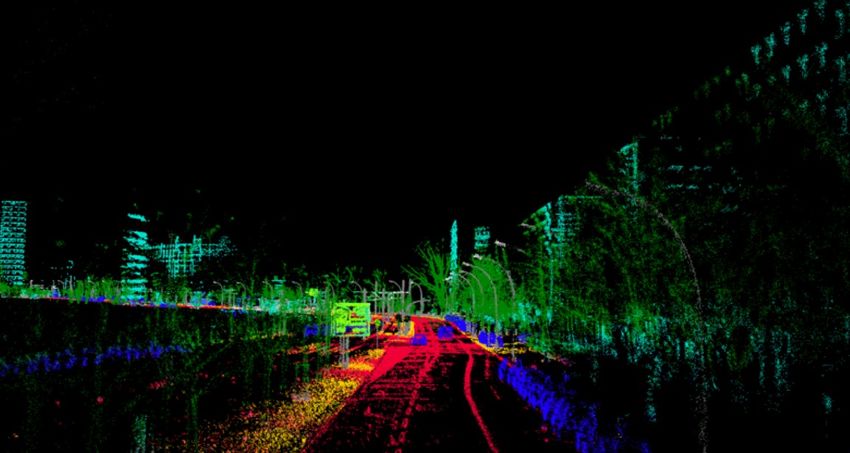
Semantic Namely, we make use of a direct sparse SLAM formula-
Segmentation
tion working on stereo images, as proposed in [19]. Here,
in a local photometric bundle-adjustment, six degrees of
Temporally
Direct Sparse
Consistent
freedom (6DoF) poses are estimated jointly with a sparse
Odometry
Labeling
3D reconstruction of the environment and optimized with
respect to a photometric energy function:
Global
Optimization
X X X p p
E= Eij + λEis . (1)
i∈F p∈Pi j∈obst (p)
Fig. 3: Semantic Mapping Pipeline. A direct VO front-end estimates
relative camera poses and a sparse 3D reconstruction of the environment In eq. (1), F is the set of all keyframes in the optimization
based on a sequence of stereo images. A segmentation module predicts dense window and Pi is the sparse set of points hosted in keyframe
2D semantic labels for the stereo camera images selected as keyframes by
the VO. Based on the VO outputs and the 2D semantic labels, temporally i. A point p ∈ Pi is defined by its fixed 2D pixel location
consistent 3D point labels are generated. Global optimization can be applied in the image and an inverse depth d which is estimated
to compensate for drift based on loop closure detection and the integration during optimization. obst (p) defines the projections of the
of RTK-GNSS measurements if available.
point p to the left images of all other keyframes in the
p
optimization window. Furthermore, Eis defines an additional
photometric energy term based on the projection of a point
in [59] and [60] make use of a LiDAR sensor for 3D
p into the corresponding right image. For further details, we
map generation and perform semantic image segmentation
refer to [18], [19].
to label the 3D points. The work presented in [61] also
Furthermore, our VO system additionally is able to tightly
makes use of LiDAR-based 3D reconstructions and image-
integrate inertial measurements from an inertial measurement
based segmentation to reconstruct both 3D semantic point
unit (IMU) if available, as described in [62]. By fusing the
clouds as well as semantic 2D occupancy grids.
VO outputs with GNSS measurements and performing loop
III. L ARGE - SCALE 3D S EMANTIC M APPING closure detection, a globally consistent 3D map is obtained.
Overall, the mapping front-end used in our pipeline is similar
The proposed 3D semantic mapping system utilizes solely to the one proposed in [7].
stereo images and optional sensor data like GNSS (Global
Navigation Satellite System) for global positioning and B. Semantic Segmentation
IMU measurements. Figure 3 shows an overview of our Semantic segmentation plays an influential role in our
semantic mapping pipeline. The direct VO module of our pipeline as it sets the baseline for the quality of our semantic
pipeline estimates relative camera poses and a sparse 3D point clouds. Since there are already plentiful excellent
reconstruction of the environment (Sec. III-A). Global map works, we build our pipeline based on them. Because of
optimization is performed based on loop closure detection. If the modularity of our pipeline, the semantic segmentation
available, RTK-GNSS measurements are integrated to obtain component consumes only images and, thus, is independent
a geo-referenced and globally accurate map. A state-of-the- of the rest of the pipeline. Therefore, any start-of-the-art
art semantic segmentation network (Sec. III-B) is used to method can be integrated into our pipeline.
generate accurate semantic labels for each pixel of the stereo In this paper, we build our pipeline based on [50]. The
images corresponding to the keyframes defined by the VO work proposed in [50] has the best performance on the KITTI
front-end. Furthermore, our temporally consistent labeling semantic segmentation benchmark [63] among all open-
module can generate temporally consistent 3D point labels source submissions. It achieves state-of-the-art performance
based on the VO outputs and the 2D semantic labels (Sec. III- by augmenting the training set with synthesised samples
C). When lifting the 3D reconstruction to a global, geo- generated by the joint image-label propagation model along
referenced, frame with GNSS data, a city-scale map can be with the boundary label relaxation strategy to make the
created by stitching together the reconstructions from a fleet model robust to noisy boundaries.
of vehicles, as shown in Figure 1. In our pipeline, the semantic segmentation module predicts
a full-resolution semantic map for each pair of images from
A. Visual Odometry and 3D Mapping the stereo cameras corresponding to the keyframes defined
The core of the proposed semantic mapping pipeline is by the VO module and then feeds the consecutive maps into
a state-of-the-art visual SLAM algorithm. To provide rich the temporally consistent labeling module (Section III-C).
information about the 3D environment, a detailed recon-
struction of the surroundings at a certain density level is C. Temporally Consistent Labeling
required. The proposed semantic mapping pipeline relies on Even though DNNs for image-based semantic segmenta-
a direct SLAM front-end for 3D map generation, which tion significantly improved over the last years, these net-
provides a much denser and more detailed reconstruction works still suffer from noise in the predicted labels as well as
of the environment compared to indirect (keypoint-based) temporal inconsistency across the estimations of a temporal
SLAM approaches. sequence of images. On one side, there are usually significant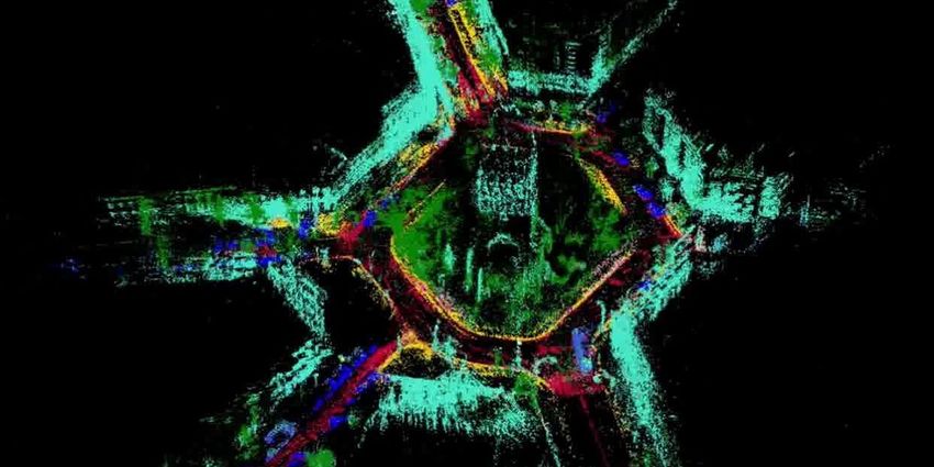
appearance changes of objects caused by the perspective                 Based on the set V , the point p gets the label with the
imaging process. On the other side, the prediction capability         highest weight assigned:
of DNNs is still developing and imperfect estimations can
often be temporal inconsistent.                                                          Li (p) ← arg max (V )                   (3)
   However, with respect to the task of autonomous driving,              In this way, point labels are obtained in consideration of
one is generally more interested in temporally consistent 3D          the temporal semantic segmentation information. As the VO
semantic labels than 2D labels in image space. Therefore,             front-end provides only a sparse set of points, the temporally
we are proposing a simple but effective scheme to obtain              consistent labels are also only provided for this set.
accurate and consistent 3D labels only from images.
   As described in Section III-A, our direct sparse VO                D. Semantic 3D Point Cloud Generation
system [18], [19] generates a sparse set of points                       The final step of our pipeline is to generate the semanti-
P := {P0 , Pi , · · · , PN } to define the 3D reconstruction.         cally labeled 3D point cloud. Based on the modules presented
Here a point p ∈ Pi is defined by the pixel coordinates               in Section III-B and Section III-C, we are able to assign
(u, v) in its host keyframe i ∈ F as well as a corresponding          semantic labels to points generated by the VO (Sec. III-A).
inverse depth d. Therefore, a point can be projected to a             Finally, these labeled 2D points are projected to 3D and
global 3D frame using the corresponding keyframe pose                 transformed to a globally consistent 3D frame forming a
ξ i ∈ se(3). In general, the tracked points are treated as            sparse 3D semantic map as the example shown in Figure 2.
statistically independent from each other. Furthermore, the
point selection scheme avoids having multiple image points                                IV. E XPERIMENTS
hosted in different frames corresponding to the same object              In the following, we evaluate our pipeline on the KITTI-
points.                                                               360 dataset [1]. We propose the generation of improved
   In the segmentation process described in Section III-B, the        ground truth semantic labels for the generated 3D points by
individual images of the sequence are treated independent             fusing labels of 2D images and 3D LiDAR points from the
from each other. While the direct VO front-end implicitly             KITTI-360 dataset. We show both quantitative and qualita-
establishes correspondences between consecutive images as             tive results and demonstrate the performance improvement
defined in eq. (1). Therefore, we can resort to these corre-          with the temporally consistent labeling. In addition to the
spondences to improve the quality of the 3D point labels.             systematic evaluations on the KITTI-360 dataset, Figure 1
   Similar to the photometric energy formulation in eq. (1),          shows the capability of our pipeline to generate a city-scale
we project each point p ∈ Pi from its host keyframe                   semantic map from data collected by a fleet of vehicles.
i to the left images corresponding to all other keyframes
j in the neighborhood in which the point p is visible                 A. Dataset
(j ∈ obst (p)) to generate a set of co-visible points cor-               KITTI-360 [1] is a large-scale dataset that covers 74 km
responding to this point. We also project this set of left            suburban traffic scenes with over 400k images and over
image points to their respective right images to obtain               100k LiDAR scans. It provides rich annotations, including
another set of corresponding points. Both sets of points              manually labeled 3D LiDAR point clouds and front-view 2D
from the left and right image stream constitute the final             semantic labels transferred from the 3D annotations.
co-visible point set. Then we define a set of C votes                    As described in Section III-A, our 3D mapping core
V := {v1 , v2 , · · · , vC } for each point p, where vc is defined    generates sparse point clouds only from images [19]. The
as an accumulated vote based on the weights wj from all               3D points generated by our pipeline differ from the LiDAR
co-visible points for one semantic class c and C is the total         points provided in the KITTI-360 dataset. Hence, it is neces-
number of classes.                                                    sary to associate our generated points with the ground truth
                                                                      provided by the KITTI-360 dataset. Then we can properly
                          (
       X                                                       −1
vc =        wj w = dj for c = Lj (q j ) and dj < distmin ,
                     j                                                evaluate the performance of our semantic mapping approach.
       j∈Q                  0 otherwise.
                                                                         Our pipeline generates point clouds solely from image
                                                                (2)   data without integrating global measurements like GNSS.
Here Q is the set of all co-visible points, including the point       Therefore, we cannot guarantee that our 3D model can be
p itself, dj is the inverse depth of a point q j and Lj is            globally aligned with the provided LiDAR points up to
the 2D semantic map corresponding to keyframe j. distmin              centimeter accuracy, even though the VO front-end provides
defines a minimum object distance. By utilizing the inverse           locally highly accurate camera poses and 3D reconstructions.
depth dj as a weighting factor for the corresponding vote,            Besides, the distribution of the points reconstructed by the
we consider the fact that predictions for points far from             VO is generally non-isotropic and highly dependent on the
the camera are generally less accurate than close points.             distance of an object point to the camera. Therefore, instead
Meanwhile, image regions for very close objects commonly              of performing global point cloud alignment, we use the
suffer from significant motion blur and strong perspective            provided ground truth poses to perform a keyframe-wise
distortion, which again results in inaccurate predictions. This       alignment between the camera-based reconstruction and the
is accounted for by setting a minimum distance threshold              LiDAR ground truth. For all points hosted in a keyframe,
distmin in the voting process.                                        we perform point matching in 2D by projecting the labeled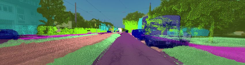
TABLE I: Evaluation results in per-class IoU and mIoU metrics of our approach on KITTI-360 dataset.

   class       road sidewalk building wall fence pole traffic light traffic sign vegetation terrain car truck bus   train motorcycle bicycle person rider   mIoU
  Baseline     94.4   79.4     86.6   54.6 34.4 39.2       6.6          45.7        90.1     60.8 83.4 71.7 89.1    91.8    46.3      19.3    36.2   4.0    58.5
 TCL Mono      95.3   83.6     87.7   63.3 42.4 47.5       9.9          51.2        91.3     64.9 83.7 77.6 92.4    92.3    55.5      37.9    64.3   5.3    63.6
 TCL Stereo    95.4   84.1     90.9   63.3 42.7 51.0      10.1          52.0        91.8     65.3 86.1 79.8 94.3    95.8    57.4      38.2    68.2   5.3    65.1

                        TABLE II: Evaluation results in class-wise mAcc and OA metrics of our approach on KITTI-360 dataset.

   class       road sidewalk building wall fence pole traffic light traffic sign vegetation terrain car truck bus   train motorcycle bicycle person rider   OA
  baseline     96.4   88.9     94.4   67.7 56.1 82.2      81.3          80.3        94.2     83.6 96.6 87.0 95.4    97.3    52.8      94.5    90.9 100.0    91.4
 TCL Mono      97.3   91.2     94.7   73.0 58.1 83.8      87.3          83.2        95.5     85.8 97.9 93.3 96.3    97.3    62.4      95.8    94.0 100.0    94.1
 TCL Stereo    97.5   91.9     95.1   73.2 59.9 84.5      87.6          83.4        95.6     85.8 98.2 93.4 98.5    98.9    64.8      97.0    94.6 100.0    95.2

Fig. 4: Label quality of 3D and 2D semantic ground truth of the KITTI-360
dataset [1] and the semantic labels we associate for our point clouds. Top        Fig. 5: Large-scale semantic map generated by the proposed pipeline. The
Left: In the green box, the points around the cars in blue are mislabeled as      figure shows the entire globally consistent reconstruction of Sequence 9 from
parking class in pink in KITTI-360 3D semantic ground truth. Bottom Left:         the KITTI-360 dataset [1] and zoomed-in sections show the fine-grained
In the red box, the building and traffic sign are mislabeled as vegetation        reconstruction details.
and in the yellow box, a mail box is mislabeled as a car in KITTI-360 2D
semantic ground truth. Top Right: The 3D semantic labels given by KITTI-
360 projected into one keyframe where the traffic light and the mail box
are not mislabeled. Bottom Right: The ground truth labels we associated
                                                                                  (TCL) module based on the pre-trained network weights1 .
for our point clouds based on the given KITTI-360 2D and 3D labels. The           For the TCL module we provide results using semantic labels
filtered points in white: the mislabeled points in red boxes, the points on       predicted only for the left camera images (Mono) as well as
the boundaries in yellow boxes, and the points in the sky in the green box.
                                                                                  using semantic labels for both left and right images (Stereo).
                                                                                    2) Measurement Metric: To evaluate the performance of
                                                                                  semantic label prediction, we follow the standard to apply
LiDAR points into the keyframe image and assigning the
                                                                                  per-class intersection-over-union (IoU) [64] and the mean
labels of LiDAR points to the matched points. We utilize
                                                                                  IoU (mIoU) metrics over all sequences.
LiDAR points up to 100 meters away from the camera, which
makes the projected points dense enough in 2D to have all                                                                                       C
                                                                                                        T Pc                                 1 X
points match a label. The top right plot in Figure 4 shows                           IoUc =                                    mIoU =              IoUc (4)
                                                                                                 T Pc + F Pc + F Nc                          C c=1
the density of the projected 3D points. Additionally, depth
information is utilized to reject false assigned point pairs.                     where T Pc , F Pc , and F Nc indicate the number of true
   In KITTI-360 dataset, the labels of the 3D points are                          positive, false positive, and false negative estimations for
generated by placing primitive cuboids and ellipsoids around                      each class c in all sequences respectively. C is the number
objects and assigning a class label to the enclosed points.                       of evaluation classes.
Besides, it focuses on static scene objects. As a result, not all                   As the number of points of each class varies prominently,
points are accurately labeled in 3D. The given 2D semantic                        we also measure the class-wise prediction mean accuracy
ground truth is derived from the 3D labels, making the 2D                         (mAcc) and the overall accuracy (OA) over all sequences:
ground truth not absolutely accurate as well. The left column                                                             PC
                                                                                                     T Pc                        T Pc
of Figure 4 shows two examples that have mislabeled objects.                                mAcc =                 OA = Pc=1  C
                                                                                                                                           (5)
Therefore, we fuse both the 2D image labels and the 3D                                                Nc                      c=1 Nc
LiDAR labels provided by the dataset to obtain reliable                           where Nc is the number of points predicted as class c.
ground truth. Only if the labels of both 2D and projected                            3) Results: Table I shows the evaluation results in per-
3D points are consistent, they are considered as ground truth                     class IoU and mIoU. Table II presents them in class-wise
for evaluation, as shown in the bottom right plot in Figure 4.                    mAcc and OA. These class-wise measurements indicate
B. Evaluation                                                                     that our approach performs well on primary static classes,
                                                                                  including road, sidewalk, building and vegetation classes,
   1) Settings: We evaluate our approach on all 9 released                        and also on some dynamic classes, car, truck, and bus
sequences of the KITTI-360 dataset. The evaluation is done                        because most objects of these classes are not moving in
on all classes as defined except the void-type classes, e.g.                      these sequences. When comparing Table I and Table II, we
unlabeled and ego vehicle, etc., and the sky class as our                         can conclude that our approach performs better in terms of
map does not contain points representing the sky. The                             precision than recall, especially on classes representing small
performance is evaluated for the baseline model presented
in Section III-B [50] and the temporally consistent labeling                         1 https://github.com/NVIDIA/semantic-segmentation/tree/sdcnet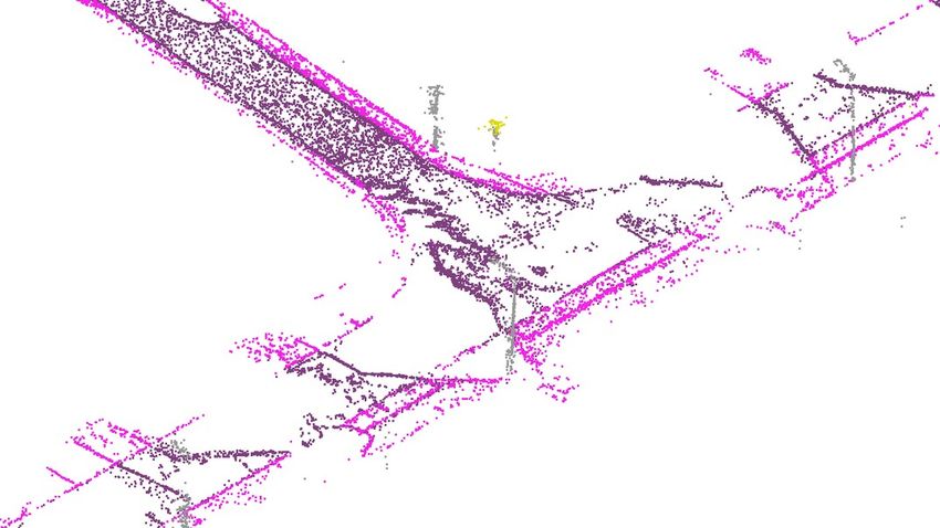
Fig. 6: Semantic point labels generated by our approach. The sparse points hosted in a keyframe are overlaid with the 2D ground truth labels and the
image from KITTI-360. This is only a subset of all points in the optimization window. Two rows represent one example, where the first and second row
shows the prediction results in full images and the zoom-in windows, respectively. Columns show (left) sparse ground truth labels, (center) labels predicted
by the baseline model, (right) labels estimated by TCL, respectively. Points which are wrongly predicted by the baseline but corrected by the TCL are
highlighted with green boxes. Points not corrected by the TCL are highlighted with red boxes.

objects, e.g. traffic sign, traffic light, bicycle, person. These                                          V. C ONCLUSION
small objects have more complex and elongated boundaries,
                                                                                   We presented a large-scale semantic mapping pipeline,
and the points near boundaries are more challenging to be
                                                                                which combines a state-of-the-art direct sparse VO front-end
perfectly classified. Besides, there are only a few points cor-
                                                                                and a back-end with global optimization and image-based
responding to the small objects, and thus a wrong prediction
                                                                                semantic segmentation. We demonstrated that predictions
can reduce the IoU and mAcc by a large margin. Thus, the
                                                                                of the semantic segmentation network could be improved
large classes has better results than the small classes.
                                                                                by incorporating temporal correspondences established by
                                                                                VO. Furthermore, we showed that our pipeline is capable
   The proposed temporally consistent labeling (TCL) fixes
                                                                                of generating city-scale semantic maps covering thousands
inconsistent predictions which mainly occur on object bound-
                                                                                of kilometers of the road by using a fleet of vehicles. Such
aries across consecutive frames. Therefore, TCL outperforms
                                                                                large-scale semantic maps can serve as intermediate results
the baseline model, especially on small objects, e.g. pole,
                                                                                towards fully vectorized HD maps. Besides, we see it as
motorcycle, bicycle, and person. Furthermore, the stereo
                                                                                a next step to build semantic 3D volumetric maps at scale
version clearly outperforms the mono version.
                                                                                with the combination of state-of-the-art dense reconstruction
                                                                                approaches like [65].
  Qualitative results of semantic point cloud labels generated
by our approach are shown in Figure 6. It illustrates how
                                                                                                       ACKNOWLEDGEMENT
TCL can improve the label estimation accuracy. Additionally,
Figure 5 shows an entire large-scale map generated by our                          We thank the entire Artisense team for their support in
approach from the sequence 9 in KITTI-360 dataset.                              setting up the pipeline and making this project happen.
R EFERENCES                                        [23] J. L. Schönberger and J.-M. Frahm, “Structure-from-motion revisited,”
                                                                                     in IEEE Conference on Computer Vision and Pattern Recognition
 [1] J. Xie, M. Kiefel, M.-T. Sun, and A. Geiger, “Semantic instance                 (CVPR), 2016.
     annotation of street scenes by 3D to 2D label transfer,” in IEEE           [24] N. Demmel, M. Gao, E. Laude, T. Wu, and D. Cremers, “Distributed
     Conference on Computer Vision and Pattern Recognition (CVPR),                   photometric bundle adjustment,” in International Conference on 3D
     2016.                                                                           Vision (3DV), 2020.
 [2] A. Geiger, P. Lenz, and R. Urtasun, “Are we ready for autonomous
                                                                                [25] J. Long, E. Shelhamer, and T. Darrell, “Fully convolutional networks
     driving? the KITTI vision benchmark suite,” in IEEE Conference on
                                                                                     for semantic segmentation,” in IEEE Conference on Computer Vision
     Computer Vision and Pattern Recognition (CVPR), 2012.
                                                                                     and Pattern Recognition (CVPR), 2015.
 [3] M. Cordts, M. Omran, S. Ramos, T. Rehfeld, M. Enzweiler, R. Be-
     nenson, U. Franke, S. Roth, and B. Schiele, “The cityscapes dataset        [26] H. Zhao, J. Shi, X. Qi, X. Wang, and J. Jia, “Pyramid scene parsing
     for semantic urban scene understanding,” in IEEE Conference on                  network,” in IEEE Conference on Computer Vision and Pattern
     Computer Vision and Pattern Recognition (CVPR), 2016.                           Recognition (CVPR), 2017.
 [4] G. Neuhold, T. Ollmann, S. Rota Bulò, and P. Kontschieder, “The           [27] L.-C. Chen, G. Papandreou, F. Schroff, and H. Adam, “Rethinking
     mapillary vistas dataset for semantic understanding of street scenes,”          atrous convolution for semantic image segmentation,” in IEEE Con-
     in International Conference on Computer Vision (ICCV), 2017.                    ference on Computer Vision and Pattern Recognition (CVPR), 2017.
 [5] J. Behley, M. Garbade, A. Milioto, J. Quenzel, S. Behnke, C. Stach-        [28] L.-C. Chen, G. Papandreou, I. Kokkinos, K. Murphy, and A. Yuille,
     niss, and J. Gall, “SemanticKITTI: A dataset for semantic scene                 “Semantic image segmentation with deep convolutional nets and fully
     understanding of lidar sequences,” in International Conference on               connected crfs,” in International Conference on Learning Representa-
     Computer Vision (ICCV), 2019.                                                   tions (ICLR), 2015.
 [6] P. Wang, X. Huang, X. Cheng, D. Zhou, Q. Geng, and R. Yang, “The           [29] A. Schwing and R. Urtasun, “Fully connected deep structured net-
     apolloscape open dataset for autonomous driving and its application,”           works,” ArXiv, 2015.
     IEEE Transactions on Pattern Analysis and Machine Intelligence             [30] S. Zheng, S. Jayasumana, B. Romera-Paredes, V. Vineet, Z. Su, D. Du,
     (TPAMI), 2019.                                                                  C. Huang, and P. H. S. Torr, “Conditional random fields as recurrent
 [7] P. Wenzel, R. Wang, N. Yang, Q. Cheng, Q. Khan, L. von Stumberg,                neural networks,” in International Conference on Computer Vision
     N. Zeller, and D. Cremers, “4Seasons: A cross-season dataset for                (ICCV), 2015.
     multi-weather SLAM in autonomous driving,” in German Conference            [31] G. Lin, C. Shen, A. van den Hengel, and I. Reid, “Efficient piecewise
     on Pattern Recognition (GCPR), 2020.                                            training of deep structured models for semantic segmentation,” in IEEE
 [8] G. Klein and D. Murray, “Parallel tracking and mapping for small AR             Conference on Computer Vision and Pattern Recognition (CVPR),
     workspaces,” in IEEE and ACM International Symposium on Mixed                   2016.
     and Augmented Reality (ISMAR), 2007.                                       [32] D. Eigen and R. Fergus, “Predicting depth, surface normals and se-
 [9] R. Mur-Artal, J. M. M. Montiel, and J. D. Tardós, “ORB-SLAM: a                 mantic labels with a common multi-scale convolutional architecture,”
     versatile and accurate monocular SLAM system,” IEEE Transactions                in International Conference on Computer Vision (ICCV), 2015.
     on Robotics (T-RO), 2015.                                                  [33] L.-C. Chen, Y. Yang, J. Wang, W. Xu, and A. Yuille, “Attention to
[10] R. Mur-Artal and J. D. Tardós, “ORB-SLAM2: An open-source                      scale: Scale-aware semantic image segmentation,” in IEEE Conference
     SLAM system for monocular, stereo and RGB-D cameras,” IEEE                      on Computer Vision and Pattern Recognition (CVPR), 2016.
     Transactions on Robotics (T-RO), 2017.                                     [34] C. Farabet, C. Couprie, L. Najman, and Y. LeCun, “Learning hier-
[11] R. Elvira, J. M. M. Montiel, and J. D. Tardós, “ORBSLAM-Atlas:                 archical features for scene labeling,” IEEE Transactions on Pattern
     A robust and accurate multi-map system,” in IEEE/RSJ International              Analysis and Machine Intelligence (TPAMI), 2013.
     Conference on Intelligent Robots and Systems (IROS), 2019.                 [35] P. H. O. Pinheiro and R. Collobert, “Recurrent convolutional neural
[12] V. Usenko, N. Demmel, D. Schubert, J. Stückler, and D. Cre-                    networks for scene labeling,” in International Conference on Machine
     mers, “Visual-inertial mapping with non-linear factor recovery,” IEEE           Learning (ICML), 2014.
     Robotics and Automation Letters (RA-L), 2020.                              [36] L.-C. Chen, G. Papandreou, I. Kokkinos, K. Murphy, and A. Yuille,
[13] C. Campos, R. Elvira, J. J. Gómez Rodrı́guez, J. M. M. Montiel,                “DeepLab: Semantic image segmentation with deep convolutional
     and J. D. Tardós, “ORB-SLAM3: An accurate open-source library for              nets, atrous convolution, and fully connected crfs,” IEEE Transactions
     visual, visual-inertial and multi-map SLAM,” IEEE Transactions on               on Pattern Analysis and Machine Intelligence (TPAMI), 2018.
     Robotics (T-RO), 2021.                                                     [37] H. Zhao, J. Shi, X. Qi, X. Wang, and J. Jia, “Pyramid scene parsing
[14] R. Mur-Artal and J. D. Tardós, “Probabilistic semi-dense mapping               network,” in IEEE Conference on Computer Vision and Pattern
     from highly accurate feature-based monocular SLAM,” in Robotics:                Recognition (CVPR), 2017.
     Science and Systems (RSS), 2015.                                           [38] W. Liu, A. Rabinovich, and A. Berg, “ParseNet: Looking wider to see
[15] T. Schöps, T. Sattler, C. Häne, and M. Pollefeys, “3D modeling on             better,” ArXiv, 2015.
     the go: Interactive 3D reconstruction of large-scale scenes on mobile
                                                                                [39] H. Noh, S. Hong, and B. Han, “Learning deconvolution network
     devices,” in International Conference on 3D Vision (3DV), 2015.
                                                                                     for semantic segmentation,” in International Conference on Computer
[16] J. L. Schönberger, E. Zheng, M. Pollefeys, and J.-M. Frahm, “Pixel-
                                                                                     Vision (ICCV), 2015.
     wise view selection for unstructured multi-view stereo,” in European
     Conference on Computer Vision (ECCV), 2016.                                [40] V. Badrinarayanan, A. Kendall, and R. Cipolla, “SegNet: A deep
[17] J. Engel, T. Schöps, and D. Cremers, “LSD-SLAM: Large-scale direct             convolutional encoder-decoder architecture for image segmentation,”
     monocular SLAM,” in European Conference on Computer Vision                      IEEE Transactions on Pattern Analysis and Machine Intelligence
     (ECCV), 2014.                                                                   (TPAMI), 2017.
[18] J. Engel, V. Koltun, and D. Cremers, “Direct sparse odometry,” IEEE        [41] O. Ronneberger, P. Fischer, and T. Brox, “U-Net: Convolutional
     Transactions on Pattern Analysis and Machine Intelligence (TPAMI),              networks for biomedical image segmentation,” in miccai, 2015.
     2018.                                                                      [42] G. Lin, A. Milan, C. Shen, and I. Reid, “RefineNet: Multi-path refine-
[19] R. Wang, M. Schwörer, and D. Cremers, “Stereo DSO: Large-scale                 ment networks for high-resolution semantic segmentation,” in IEEE
     direct sparse visual odometry with stereo cameras,” in International            Conference on Computer Vision and Pattern Recognition (CVPR),
     Conference on Computer Vision (ICCV), 2017.                                     2017.
[20] N. Yang, L. von Stumberg, R. Wang, and C. Cremers, “D3VO: Deep             [43] T. Pohlen, A. Hermans, M. Mathias, and B. Leibe, “Full-resolution
     depth, deep pose and deep uncertainty for monocular visual odometry,”           residual networks for semantic segmentation in street scenes,” in IEEE
     in IEEE Conference on Computer Vision and Pattern Recognition                   Conference on Computer Vision and Pattern Recognition (CVPR),
     (CVPR), 2020.                                                                   2017.
[21] X. Gao, R. Wang, N. Demmel, and D. Cremers, “LDSO: Direct sparse           [44] J. Fu, J. Liu, Y. Wang, and H. Lu, “Stacked deconvolutional network
     odometry with loop closure,” in IEEE/RSJ International Conference               for semantic segmentation,” IEEE Transactions on Image Processing,
     on Intelligent Robots and Systems (IROS), 2018.                                 2017.
[22] M. Gladkova, R. Wang, N. Zeller, and D. Cremers, “Tight integration        [45] J. Fu, J. Liu, H. Tian, Z. Fang, and H. Lu, “Dual attention network
     of feature-based relocalization in monocular direct visual odometry,” in        for scene segmentation,” in IEEE Conference on Computer Vision and
     IEEE International Conference on Robotics and Automation (ICRA),                Pattern Recognition (CVPR), 2019.
     2021.                                                                      [46] Z. Huang, X. Wang, L. Huang, C. Huang, Y. Wei, H. Shi, and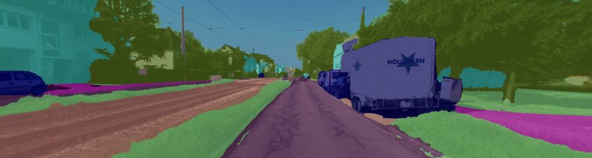
W. Liu, “CCNet: Criss-cross attention for semantic segmentation,” in
       International Conference on Computer Vision (ICCV), 2019.
[47]   Y. Yuan, L. Huang, J. Guo, C. Zhang, and X. Chen, “OCNet: Object
       context for semantic segmentation,” International Journal of Computer
       Vision (IJCV), 2021.
[48]   A. Tao, K. Sapra, and B. Catanzaro, “Hierarchical multi-scale attention
       for semantic segmentation,” ArXiv, 2020.
[49]   C. Yu, J. Wang, C. Peng, C. Gao, G. Yu, and N. Sang, “Learning a
       discriminative feature network for semantic segmentation,” in IEEE
       Conference on Computer Vision and Pattern Recognition (CVPR),
       2018.
[50]   Y. Zhu, K. Sapra, F. A. Reda, K. J. Shih, S. Newsam, A. Tao, and
       B. Catanzaro, “Improving semantic segmentation via video propaga-
       tion and label relaxation,” in IEEE Conference on Computer Vision
       and Pattern Recognition (CVPR), 2019.
[51]   A. Iscen, G. Tolias, Y. Avrithis, and O. Chum, “Label propagation
       for deep semi-supervised learning,” in IEEE Conference on Computer
       Vision and Pattern Recognition (CVPR), 2019.
[52]   Y. Zou, Z. Yu, B. V. Kumar, and J. Wang, “Unsupervised domain
       adaptation for semantic segmentation via class-balanced self-training,”
       in European Conference on Computer Vision (ECCV), 2018.
[53]   Y. Li, L. Yuan, and N. Vasconcelos, “Bidirectional learning for
       domain adaptation of semantic segmentation,” in IEEE Conference
       on Computer Vision and Pattern Recognition (CVPR), 2019.
[54]   B. Wu, A. Wan, X. Yue, and K. Keutzer, “SqueezeSeg: Convolutional
       neural nets with recurrent CRF for real-time road-object segmentation
       from 3D LiDAR point cloud,” in IEEE International Conference on
       Robotics and Automation (ICRA), 2018.
[55]   Y. Wang, T. Shi, P. Yun, L. Tai, and M. Liu, “PointSeg: Real-time
       semantic segmentation based on 3D lidar point cloud,” 2018.
[56]   L. Tchapmi, C. Choy, I. Armeni, J. Gwak, and S. Savarese, “SEG-
       Cloud: Semantic segmentation of 3D point clouds,” in International
       Conference on 3D Vision (3DV), 2017.
[57]   S. Sengupta, P. Sturgess, L. Ladicky, and P. H. S. Torr, “Auto-
       matic dense visual semantic mapping from street-level imagery,” in
       IEEE/RSJ International Conference on Intelligent Robots and Systems
       (IROS), 2012.
[58]   S. Sengupta, E. Greveson, A. Shahrokni, and P. H. S. Torr, “Urban
       3D semantic modelling using stereo vision,” in IEEE International
       Conference on Robotics and Automation (ICRA), 2013.
[59]   I. Kostavelis and A. Gasteratos, “Semantic mapping for mobile
       robotics tasks: A survey,” Robotics and Autonomous Systems, 2015.
[60]   D. Maturana, P.-W. Chou, M. Uenoyama, and S. Scherer, “Real-time
       semantic mapping for autonomous off-road navigation,” in Interna-
       tional Conference on Field and Service Robotics (FSR), 2017.
[61]   D. Paz, H. Zhang, Q. Li, H. Xiang, and H. I. Christensen, “Probabilis-
       tic semantic mapping for urban autonomous driving applications,” in
       IEEE/RSJ International Conference on Intelligent Robots and Systems
       (IROS). IEEE, oct 2020.
[62]   L. von Stumberg, V. Usenko, and D. Cremers, “Direct sparse visual-
       inertial odometry using dynamic marginalization,” in IEEE Interna-
       tional Conference on Robotics and Automation (ICRA), 2018.
[63]   H. Alhaija, S. Mustikovela, L. Mescheder, A. Geiger, and C. Rother,
       “Augmented reality meets computer vision: Efficient data generation
       for urban driving scenes,” International Journal of Computer Vision
       (IJCV), 2018.
[64]   M. Everingham, S. M. Eslami, L. Gool, C. K. Williams, J. Winn,
       and A. Zisserman, “The pascal visual object classes challenge: A
       retrospective,” in International Journal of Computer Vision (IJCV),
       2015.
[65]   F. Wimbauer, N. Yang, L. von Stumberg, N. Zeller, and D. Cre-
       mers, “MonoRec: Semi-supervised dense reconstruction in dynamic
       environments from a single moving camera,” in IEEE Conference on
       Computer Vision and Pattern Recognition (CVPR), 2021.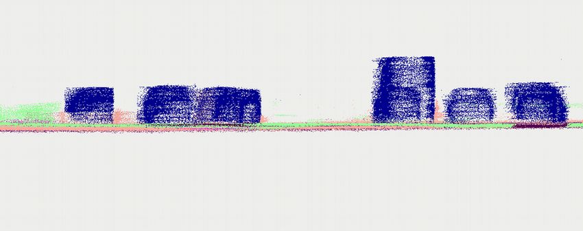
You can also read


