Properties of the lunar gravity assisted transfers from LEO to the retrograde GEO
←
→
Page content transcription
If your browser does not render page correctly, please read the page content below
www.nature.com/scientificreports
OPEN Properties of the lunar gravity
assisted transfers from LEO
to the retrograde‑GEO
Bo‑yong He*, Peng‑bin Ma & Heng‑nian Li
The retrograde geostationary earth orbit (retro-GEO) is an Earth’s orbit. It has almost the same orbital
altitude with that of a GEO, but an inclination of 180°. A retro-GEO monitor-satellite gives the GEO-
assets vicinity space-debris warnings per 12 h. For various reasons, the westward launch direction is
not compatible or economical. Thereby the transfer from a low earth orbit (LEO) to the retro-GEO via
once lunar swing-by is a priority. The monitor-satellite departures from LEO and inserts into the retro-
GEO both using only one tangential maneuver, in this paper, its transfer’s property is investigated. The
existence of this transfer is verified firstly in the planar circular restricted three-body problem (CR3BP)
model based on the Poincaré-section methodology. Then, the two-impulse values and the perilune
altitudes are computed with different transfer durations in the planar CR3BP. Their dispersions
are compared with different Sun azimuths in the planar bi-circular restricted four-body problem
(BR4BP) model. Besides, the transfer’s inclination changeable capacity via lunar swing-by and the
Sun-perturbed inclination changeable capacity are investigated. The results show that the two-
impulse fuel-optimal transfer has the duration of 1.76 TU (i.e., 7.65 days) with the minimum values
of 4.251 km s−1 in planar CR3BP, this value has a range of 4.249–4.252 km s−1 due to different Sun
azimuths in planar BR4BP. Its perilune altitude changes from 552.6 to 621.9 km. In the spatial CR3BP,
if the transfer duration is more than or equal to 4.00 TU (i.e., 17.59 days), the lunar gravity assisted
transfer could insert the retro-GEO with any inclination. In the spatial BR4BP, the Sun’s perturbation
does not affect this conclusion in most cases.
As we known, the geostationary earth orbit (GEO) has the same period as the Earth’s rotation period. Its sub-
point coverage is almost still. Many important satellites for navigation, remote sensing, data-relay, meteorology,
ocean monitoring and land-resources monitoring are deployed on the GEO. For decades, due to the exponential
growth of the number of the GEO satellites, the rocket terminal stage, the failed-satellites, the space debris, and
the safety box limitation to accommodate perturbation, many important GEO positions deploys satellites under
collocation strategy1. The circumstance of the GEO-assets is serious about the quite crowded GEO-belt. On July
28, 2014 and August 19, 2016, the USA successfully launched four GEO satellites, GSSAP-1/2 and GSSAP-3/4
(Geosynchronous space Situational Awareness-Ness Program), r espectively2. They are possible to give a few
of these GEO-assets vicinity early debris-warning by raising or lowering their orbital altitudes, but their orbit
maneuver fuel-cost greatly limits their patrol-range. The retrograde GEO (retro-GEO) is an earth’s orbit, which
has almost the same orbital altitude with that of a GEO, but an inclination of 180°. A monitor-satellite on the
retro-GEO gives all of the GEO-assets vicinity debris-warning per 12 h. The transfer from a low earth orbit (LEO)
to the retro-GEO via once lunar swing-by is shown in Fig. 1. This lunar gravity assisted manner avoids the dif-
ficulty that the number of the ground-measurement and tracks facilities is a few for westward-launch directly. In
respect that the usual space launch rocket has an eastward-launch scenarios, in this way, it saves the launching
energy-cost via the Earth’s rotation force.
The dynamics description of the lunar swing-by orbit could date back to Issac Newton in 1687. The circum-
lunar free-return orbit in Apollo mission is a famous practical activity to improve the safety of the crews in the
manned space missions3. The probe Hiten launched by Japan in 1990 acted a double lunar swing-by space-flight4.
In 1998, Hughes saved the original ISEE-3/ICE via multi-lunar swing-by and multi-maneuvers. It becomes the
first successful space legend of saving satellites5. Zeng et al.6 studied the lunar swing-by transfer using a simpli-
fied double two-body hypothesis orbital model, the transfer launches up from a high-latitude launch-pad and
transfers to the retro-GEO. His result shows that the transfer via lunar swing-by saves maneuver fuel-cost, but
State Key Laboratory of Astronautic Dynamics (ADL), Xi’an Satellite Control Center, Xi’an 710043, China. *email:
heboyong@yeah.net
Scientific Reports | (2021) 11:18813 | https://doi.org/10.1038/s41598-021-98231-1 1
Vol.:(0123456789)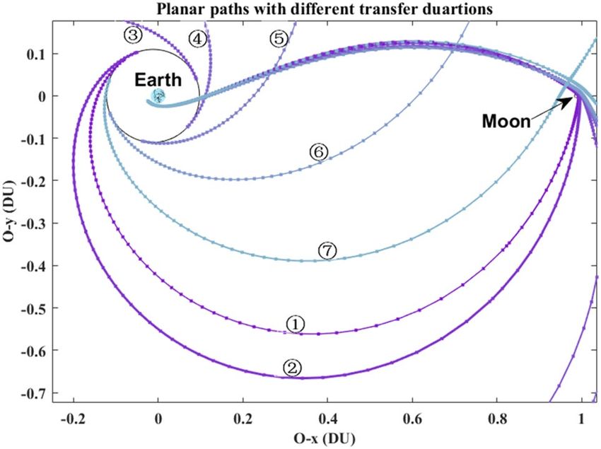
www.nature.com/scientificreports/
Retro-GEO
Transfer
LEO
Moon
Figure 1. The transfer from LEO to the retrograde-GEO via lunar swing-by.
the orbital perigee altitude and the inclination during the return retro-GEO phase in his work did not match the
retro-GEO. Luo et al.7 described the mechanics of the double-lunar swing-by, expatiated the sensitive property
of the trajectories for deep-space exploration via lunar swing-by to a certain extent.
As the number of the GEO satellites grows exponentially, the GEO-assets’ safety problem caused by the
abandoned-satellites and space-debris is becoming more and more s erious8. In fact, Oberg9 presented the pio-
neering retro-GEO concept as early as 1984, and explained the flight-manner saves fuel-cost to deploy a satellite
on the retro-GEO via lunar swing-by. Kawase et al.10,11 advanced the reasonable proposal that a monitor-satellite
on the retro-GEO plays the debris-warning alertor for all of the GEO-assets. Aravind et al.12 compared the
same satellite’s left fuel by several different typical-flight sceneries from an LEO to the final retro-GEO. Aravind
also tried to calculate the final left-fuel using lunar swing-by to compare with the typical-flight sceneries, but
the orbital perigee altitude during the return retro-GEO phase is 124.75 km, the value is far below the desired
retro-GEO orbital altitude.
To sum up, the retro-GEO monitor-satellite gives all of the GEO-assets vicinity debris-warning per 12 h, and
the flight-manner via lunar swing-by saves fuel-cost. But, the analysis of examples until now in r eferences6,12
did not satisfy the orbital element constraints. In this paper, the purpose is to discover the fundamental proper-
ties of the transfers in the classical circular restricted three-body problem (CR3BP) model and the bi-circular
four-body problem (BR4BP) model, such as, whether the transfer via lunar swing-by with the orbital element
constraints (i.e., Its orbital altitude and inclination during the departure LEO and insert retro-GEO phase) and
the two-impulse tangential maneuvers is existed or not? What is the foundational feature of this transfer in the
planar model? How much is the lunar gravity assisted effect for the orbital inclination changeable capacity? After
the concise statement of the problem in “Problem statement”, the first two questions are exhibited in “Properties
in the planar model”, and the last question is exhibited in “Properties in the spatial model”. The paper ends with
“Conclusions” which gives some brief conclusions and implications on this topic.
Problem statement
Advantages via lunar swing‑by. If the retro-GEO satellite is deployed directly by the westward-launch
manner for China, there are two problems. First, the most satellites of China launched up via an eastward-launch
manner, there is no conventional landing area for the first and second stage-debris of the westward-launch
rockets. The sub-points of the first and second stage-debris of the westward-launch rocket may spread to the
densely populated area and even out of border. Second, the eastward-launch manner can be accurately meas-
ured and controlled by the mature ground stations of China Xi’an Satellite Control Center, while the westward-
launch cannot be supported by mature ground stations. Moreover, the equatorial radius of the Earth is about
6378.134 km, and its rotation angular velocity is about 7.292115 ×10⁻⁵ rad s−1. The beneficial velocity-increment
of the eastward-launch manner launched-up from the equator is about 465 m s−1, while there is about additional
465 m s−1 velocity-increment needs to be overcome by the westward-launch manner. It is an obvious contrast to
the two manners’ fuel-cost.
The moon is the Earth’s sole natural celestial body and is the most man-made probes visited celestial body
by-far. In particular, the Chang’E-series lunar probes of China show that China has mastered the techniques of
the lunar probes launch-up, precise orbit determination, and orbital control around the Moon13.
Orbital dynamics and constraints. The most classical orbital model of describing a probe’s path in the
Earth-Moon space is the CR3BP model. In CR3BP, there are two primary bodies [P1 , P2 ] and the probe P of
masses m1 > m2 ≫ m, respectively. The motion of [P1 , P2 ] is not affected by the probe P , and move around their
common center of mass under their mutual gravity. In the Earth-Moon space, [P1 , P2 ] represent the Earth and
the Moon, respectively. Let µ = m2 (m1 + m2 ) denotes the mass ratio of P2 to the total mass. The motion of the
probe P relative to a co-rotating coordinate system O−xyz as shown in Fig. 2 with the origin at their common
center, and in normalized distance, mass, time units, and speed unit are listed in Table 1.
R3BP15 is
The differential equation description of C
∂�3 ∂�3 ∂�3
ẍ − 2ẏ = , ÿ + 2ẋ = , z̈ = . (1)
∂x ∂y ∂z
Here, the effective potential function is
1 2
1−µ µ 1
�3 = x + y2 + z 2 + + + µ(1 + µ), (2)
2 r1 r2 2
Scientific Reports | (2021) 11:18813 | https://doi.org/10.1038/s41598-021-98231-1 2
Vol:.(1234567890)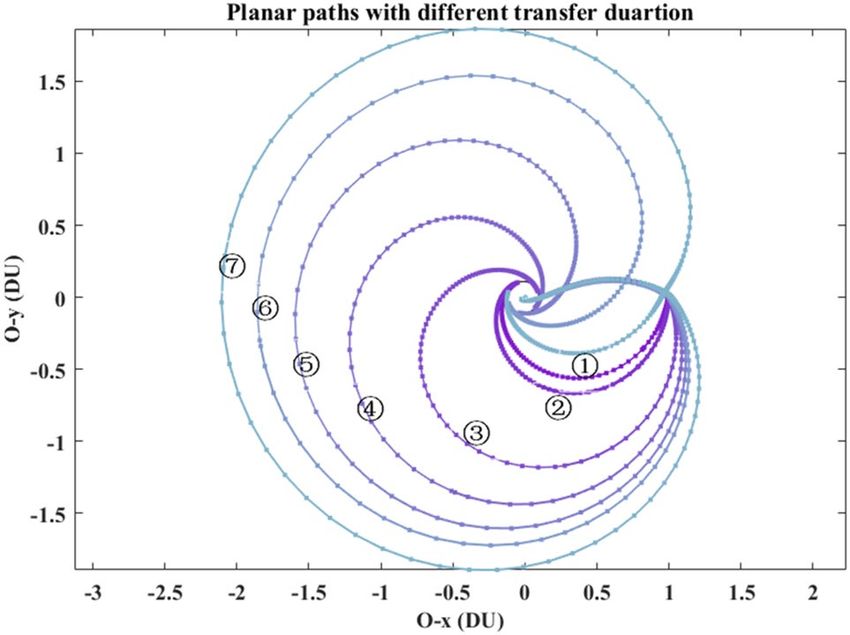
www.nature.com/scientificreports/
Z z′
ϕ0
z
z′
OE V0
O y′
R0 ϕ θ0
Moon x
X
0 y′ λ0
x′ λ0
y Y
Figure 2. The vectors of the position and velocity at the epoch of trans-lunar injection.
Symbol Value Units Meaning
µ 1.21506683 × 10⁻² – The mass ratio of the moon to the earth
ms 3.28900541 × 10⁵ – Scaled mass of the sun
ρ 3.88811143 × 10² – Scaled Sun–(earth + moon) distance
ωs − 9.25195985 × 10⁻¹ – Scaled angular velocity of the sun
lem 3.84405000 × 10⁸ m Earth–moon distance
ωem 2.66186135 × 10⁻⁶ s−1 Earth–moon angular velocity
R0 6378 km Mean earth’s radius
Rf 1738 km Mean moon’s radius
h0 167 km Altitude of departure orbit
hf 35,786 km Altitude of arrival orbit
DU 3.84405000 × 10⁸ m Distance unit
TU 4.34811305 days Time unit
VU 1.02323281 × 10³ m s−1 Velocity unit
Table 1. Earth-moon space constants14.
with r1 = (x + µ)2 + y 2 + z 2 ,r2 = (x + µ − 1)2 + y 2 + z 2 in (2). [P1 , P2 ] are located at (−µ, 0, 0) ,
(1 − µ, 0, 0), respectively.
Select the moment of the trans-lunar injection (i.e., the subscript ‘0’ means the start epoch) as the epoch of
the Earth-centered instantaneous inertial coordinate system OE - XYZ, OE - X points to the center of the Moon,
OE - Z points to the angular-momentum direction of the Moon’s path, OE - Y constructs the Cartesian coordi-
nate system with the other two axis. In the frame of OE - XYZ , the position and velocity vectors of [R0 , V 0 ] are
described as (3).
R0 = R0 · M z (− 0 )M y (ϕ0 ) · � 1 0 0 �T
(3)
V = V · M (− )M (ϕ ) · � 0 cos θ sin θ �T .
0 0 z 0 y 0 0 0
Here, R0 and V0 describe the values of the position and velocity, respectively. 0 and ϕ0 describe the position
vector. θ0 describes the direction of the velocity vector in the plane of the position vector. M y and M z are the
fundamental coordinate transformation matrixes, the other one M x does not be used here. The obvious con-
straint is satisfied as dot(R0 , V 0 ) = 0 means that the trans-lunar injection impulse is tangential to the position
vector at that epoch.
In CR3BP, O denotes the origin of the co-rotating coordinate system O−xyz . O−x follows the direction of
the Moon’s center. O−z follows the angular-momentum direction of the Moon’s path. O−y constructs the active
Cartesian coordinate system with the other two axes. The vectors of the position and velocity in O−xyz have
constraints as (4).
T
R0 = r 0 + µ 0 0
(4)
V 0 = v 0 +ω × r 0 .
T
T
T
Here, r 0 = x, y, z 0 , v 0 = ẋ, ẏ, ż 0 , ω = ωx , ωy , ωz = [0, 0, 1]T . And the additional rotation velocity is
Scientific Reports | (2021) 11:18813 | https://doi.org/10.1038/s41598-021-98231-1 3
Vol.:(0123456789)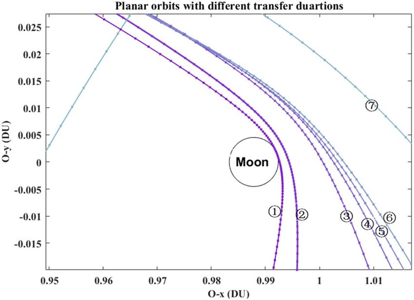
www.nature.com/scientificreports/
Figure 3. The select Poincaré section.
0 −ωz ωy
ω × r0 = ωz 0 −ωx r 0 . (5)
−ωy ωx 0
Select the epoch of the perigee during the return retro-GEO phase as the final moment (i.e., the subscript
‘f ’ means the final). The position vector and the velocity vector satisfy the constraint of dot(Rf , V f ) = 0 at this
epoch. Besides, another constraint is that the perilune altitude of the transfer is more than zero at least.
A more precise orbit model is the BR4BP model. BR4BP considers the four-body P3 base on CR3BP. In the
Earth–Moon space, P3 denotes the Sun. The Sun-perturbed orbital dynamics model of P16 is
∂�4 ∂�4 ∂�4
ẍ − 2ẏ = , ÿ + 2ẋ = , z̈ = . (6)
∂x ∂y ∂z
The moon orbit inclination on the ecliptic is about 5°, the planar BR4BP catches basic insights of the real
four-body dynamics17. The equivalent potential function is
ms ms
�4 x, y, z, t = �3 x, y, z + − 2 x cos (ωs t) + y sin (ωs t) . (7)
r (t) 3 ρ
Here, ms denotes the scaled mass of the Sun. ρ denotes the scaled the Sun and the Earth–Moon barycenter dis-
tance. ωs denotes the angular velocity of the Sun in the Earth–Moon rotating frame. The phase angle of the Sun
to the O − x axis is ωs t at the moment. Hence the position of the Sun is (ρ cos (ωs t), ρ sin (ωs t)). The distance
from the lunar probe P to the Sun is
2
r3 (t) = (x − ρ cos (ωs t))2 + y − ρ sin (ωs t) . (8)
Properties in the planar model
Existence verification. Considering that the transfers solved by the previous w
orks6,12 did not completely
satisfy the constraints (i.e., two tangential maneuvers and the perigee altitude during the return retro-GEO
phase), its existence need to be firstly verified. Poincaré proves that there is no general analytical mathematical
procedure of computing the transfers in the three-body problem. He suggested the Poincaré section methodol-
ogy to formulate the property of the multidimensional nonlinear differential equations. This methodology gives
a clear criterion and qualitative conclusion for these problems. The planar CR3BP is a dimension-reduced result
of (1), the O − z direction is decoupled from the other two directions in O − xyz . To be specific, the orbital
element [ϕ, θ ] are zero in the full time. In this paper, it is used flexibly to obtain the transfer’s existence features.
Select the orbital elements both at the moment of trans-lunar injection and at the moment of the perigee dur-
ing the return retro-GEO phase as the traversal searching variables. The trans-lunar phase is computed using the
numerical integration by the positive direction of time, while the return retro-GEO phase is computed using the
numerical integration by the negative direction of time. Both stop at the Poincaré section. The Poincaré section
is selected here at the axis of O − x and is far-side from the Earth and the Moon. It has three orbital elements as
shown in Fig. 3, the position on O − x of xp, the velocity value of vp, and the velocity angle of ξp. All of them is
at the epoch when the position component of O − y is zero (i.e., yp = 0). The subscript ‘p’ denotes this moment
just because it is close to the perilune epoch.
The geocentric distance R0 at the epoch of trans-lunar injection is a constant, because it is dominated by the
capability of the rocket. The geocentric distance Rf at the moment of the perigee during the return retro-GEO
phase is the same with that of the GEO. This transfer’s existence validation converts into an appointment at the
selected Poincaré section as expressed
+ in Fig.
4.
−
The orbital elements xp , vp , ξp and xp , vp , ξp , which are computed from [R0 , 0 , V0 ] and [Rf , f , V
f ],
+
respectively, meet
− at the Poincaré section of yp = 0. If there is a non-empty intersection set about xp , vp , ξp
and xp , vp , ξp , this transfer’s existence is sufficiently validated. Otherwise, there is no transfer satisfied the
constraints in “Orbital dynamics and constraints” in the planar CR3BP.
Scientific Reports | (2021) 11:18813 | https://doi.org/10.1038/s41598-021-98231-1 4
Vol:.(1234567890)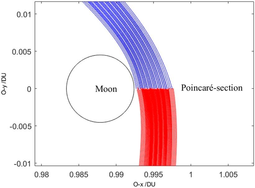
www.nature.com/scientificreports/
Figure 4. Illustration of the existence validation strategy.
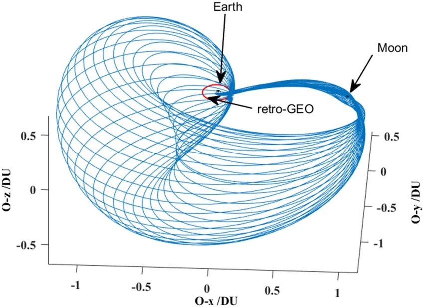
Figure 5. The planar trajectories of the transfers.
Computing orbit elements Results of Poincaré-section map
Symbol Value (units) Symbol Value (units)
R0 6545 (km) xp+ [0.9926,0.9975] (DU)
0 [225.1, 225.4] (°) vp+ [0.3377,0.5615] (VU)
V0 [10.9838, 10.985] (km s−1) ξp+ [− 82.4637, −73.9266] (°)
Rf 42,164 (km) xp− [0.9928, 0.9976] (DU)
f [126.5, 127.3] (°) vp− [0.3190, 0.6998] (VU)
Vf [4.1261, 4.1271] (km s−1) ξp− [− 81.4566, − 74.6909] (°)
Table 2. The orbital elements of plotting the Poincaré section.
Without loss of generality, set R0 = 6545 km (i.e., 6378 + 167)14, and set Rf = 42,164 km (i.e. 6378 + 35,786).
The orbital elements of plotting all of the trajectories in Fig. 5 are listed in Table 2. Its partial detail trajectories
enlarged of the Poincaré section are plotted in Fig. 6. The Poincaré
+ section’s three plane views are plotted in
Fig. 7a–d. The blue square
− is the trans-lunar phase of xp , vp , ξp while the red pentagram is the return retro-
GEO phase of xp , vp , ξp .
It shows clearly that the Poincaré section is a non-empty set, the transfer’s existence is validated. The transfer
exists, which is from an LEO of deploying the retro-GEO via lunar swing-by with two tangential maneuvers.
Optimal two‑impulse solution. In the planar CR3BP, the optimal two-impulse solution is the usual com-
puting goal. The continuation theory is practically useful to solve the transfer which has some sensitive design
uration14,18. From the primary computing results of the Poincaré section in “Existence verifi-
variables or a long d
cation”, some solutions give the goal the initial value of the orbital elements. Then, a continuation frame is built.
This frame employs the duration of the transfer plays the role of the continuation element as (9) in the outer
layer.
for �t�= �tmin : �tstep : �tmax
x = [ 0 , V0 , f , Vf ]
Outer Inner min J = �v (9)
s. t. ε = 0
end
Scientific Reports | (2021) 11:18813 | https://doi.org/10.1038/s41598-021-98231-1 5
Vol.:(0123456789)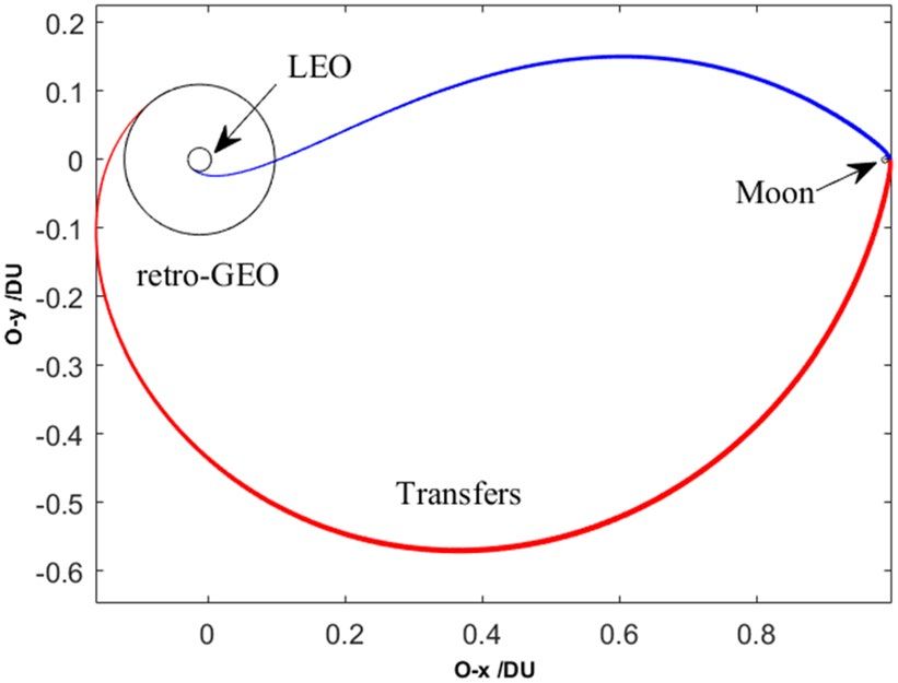
www.nature.com/scientificreports/

                                            Figure 6.  The partial enlarged detail of the Poincaré-section.

                                            Figure 7.  The three-dimensional parameter of the Poincaré section.

          Scientific Reports |   (2021) 11:18813 |               https://doi.org/10.1038/s41598-021-98231-1       6

Vol:.(1234567890)
www.nature.com/scientificreports/
Figure 8. Two-impulse value and perilune altitude vs. transfer-duration.
No ① ② ③ ④ ⑤ ⑥ ⑦
t (TU) 1.55 1.76 3.00 4.00 5.00 5.94 7.00
v (km s−1) 4.2588 4.2509 4.3106 4.3455 4.3622 4.3695 4.3144
hprl (km) 2.6534 590.16 2349.1 2759.1 2880.1 3080.6 7054.0
Table 3. The two-impulse values and its perilune altitudes.
The step value of tstep can be adjusted as needed (e.g., the optimal iteration convergence performance).
In the inner layer, there is just a simple constrained optimization model. The sum of the two-impulse of v is
optioned as the minimum objective. Its expression is
�v = V0 − µE R0 + Vf − µE Rf . (10)
Here, µE = 398600.44 km3 s−1. To be the same with the design variables in “Existence verification”, [ 0 , V0 , f , Vf ]
18
plays the role of the variables. Refer to our
previous work experience
, slice the total transfer duration into two
segments, tmid denotes the middle epoch. x�mid , y�mid , ẋ�mid
, �mid denotes the flight state which is computed from
ẏ
← ← ← ←
the LEO by the forward-time numerical integration. x , y , ẋ mid , ẏ mid denotes the flight state which is
mid mid
computed from the retro-GEO by the reverse-time numerical integration. Under ideal condition,
← ← ← ←
� �
x�mid , y�mid , ẋmid , ẏmid ≡ x , , ẋ mid , ẏ mid . But small numerical integration error ε exists in the actual
y
mid mid
numerical calculation. It will be made up by a mid-course correction in the engineering project.
← ← ←
←
ε= x�mid , y�mid , ẋ�mid , ẏ�mid − x , y , ẋ mid , ẏ mid .
(11)
mid mid
The sequence quadratic programming (SQP) algorithm in the Matlab fmincon function is applied for the
inner layer in this paper. Here, the value of ε is limited to 1 × 10⁻⁴, otherwise, it is considered that the two phases
cannot be joined. Addition, another potential constraint is that the value of the perilune altitude hprl must be
more than zero. The optimal two-impulse solution is shown in Fig. 8.
It can be seen that when the transfer duration approaches to 7 TU, the value of ε is more than 1 × 10⁻⁴ .
With the increasing of the transfer duration, the value of the perilune altitude always increases. The optimal
two-impulse value, v = 4.2509 km s−1, occurs at the case that the duration is 1.76 TU (i.e., 7.65 days). While
its maximum value, v = 4.3695 km s−1, occurs at the case that the duration is 5.94 TU (i.e., 25.83 days). The
detail elements of the seven solutions marked in Fig. 8 are listed in Table 3.
These seven planar paths with different transfer duration are plotted in Fig. 9. Its detailed paths in the Earth
vicinity and in the Moon vicinity are shown in Fig. 10 and in Fig. 11, respectively. The rkf-78 numerical integrator
is used and its step size is 2 × 10⁻², so the markers of these paths are not uniform.
We all know that the Sun’s perturbation affects the transfer in the BR4BP. This time, the transfer duration
t is a constant, but the Sun’ azimuth plays the role of the continuation element to construct a frame as (12).
Scientific Reports | (2021) 11:18813 | https://doi.org/10.1038/s41598-021-98231-1 7
Vol.:(0123456789)www.nature.com/scientificreports/
Figure 9. The planar paths in the overall view.
Figure 10. The detail paths in the Earth vicinity.
Figure 11. The detail paths in the Moon vicinity.
Scientific Reports | (2021) 11:18813 | https://doi.org/10.1038/s41598-021-98231-1 8
Vol:.(1234567890)www.nature.com/scientificreports/
Figure 12. Two-impulse value and perilune altitude oscillate in the planar BR4BP.
Figure 13. Two-impulse value and perilune altitude oscillate with different transfer duration.
min : θ step : θmidmax
for θmid = θmid mid
x = [ 0 , V0 , f , Vf ]
�
Outer Inner min J = �v (12)
s. t. ε = 0
end
Here, θmid = ωs · tmid . tmid is the middle epoch of the transfer duration. When θmid changes from zero to 2π, the
two-impulse value and the perilune altitude oscillate as plotted in Fig. 12.
The cumulative effect of the solar perturbation is obvious with the transfer duration increasing. In the case
of t = 1.76 TU, v has a range of [4.2489, 4.2521] km s−1, hprl has a range of [552.61, 621.90] km. The transfer
duration changes 0.01 TU (i.e., about 1 h), the value of v is almost unchanged while the value of hprl has a dif-
ference of about 24.5 km. The detail difference is shown in Fig. 13.
Properties in the spatial model
Inclination changeable capacity via lunar swing‑by. The original intention of this transfer via lunar
swing-by is of changing the orbital inclination from a direct LEO to a retro-GEO orbit at the Earth-centric view.
The orbital inclination changeable capacity via lunar swing-by is investigated in this Section. Based on the solu-
tions in the planar model, the solution in the spatial model is easy to be calculated also using the continuation
strategy as (13).
step step
for θf �
= π : θf : 2π && θf = π : −θf : 0
x = [ 0 , ϕ0 , V0 , θ0 , �t, f , ϕf , Vf ]
Outer Inner min J = �v (13)
s.t. ε = 0
end
In the planar CR3BP, the value of θf is a constant of π . It’s the most important element which affects is inclina-
tion of inserting the retro-GEO. Here, it plays the role of the continuation element. Its value changes from π to
both zero and 2π in parallel. The solutions which satisfy the limit value of ε ≤ 1 × 10⁻⁴ are plotted as Fig. 14.
It displays the symmetrical features of the transfers in the spatial CR3BP model as proven by Ref.19. In order
to express the relationship between the inclination changeable capacity and the transfer duration more clearly,
the solutions of t = 2.00 TU and t = 2.50 TU are supplemented. When t is more than 4.00 TU, just via lunar
Scientific Reports | (2021) 11:18813 | https://doi.org/10.1038/s41598-021-98231-1 9
Vol.:(0123456789)www.nature.com/scientificreports/
Figure 14. Inclination changeable capacity in the spatial CR3BP.
t (TU) 1.55 1.76 2.00 2.50 3.00 4.00 5.00 5.94
θfmin (°) 113 87 82 50 25 0 0 0
θfmax (°) 247 273 278 310 335 360 360 360
v (km s−1) 4.2438 4.2173 4.2099 4.1830 4.1939 4.2294 4.2601 4.2905
Table 4. The inclination changeable capacity and the transfer duration.
Figure 15. Perilune altitude changes in the spatial CR3BP.
swing-by, the transfer could insert the retro-GEO with any inclination value. The detail values of the inclination
changeable capacity with the transfer duration are listed in Table 4.
In addition to this, the perilune altitudes of them are all more than zero. The validating data is plotted as
shown in Fig. 15.
Here, all the spatial paths of the case that t= 4.00 TU are exhibited in Fig. 16. These spatial paths constitute
an envelope.
Sun‑perturbed inclination changeable capacity. Set t and θf as constants in the spatial BR4BP, the
Sun-perturbed inclination changeable capacity is exhibited by traversing all the Sun’s azimuths based on the
solution in the planar CR4BP. The result is shown as Fig. 17.
In the most of the cases, ε could approach the limited value of 1 × 10⁻⁴ . But in the case which t= 4.00 TU
and θf = 50°, when θmid is near to 130° and 310°, the value of ε reaches 6.9 ×10⁻³. The three axial paths comparison
is shown in Fig. 18. It serves to show that the Sun’s perturbation difference occurs mainly in the O−xy planar.
Scientific Reports | (2021) 11:18813 | https://doi.org/10.1038/s41598-021-98231-1 10
Vol:.(1234567890)www.nature.com/scientificreports/
Figure 16. All the spatial paths of the case that t= 4.00 TU.
Figure 17. The value of ε with different Sun’ azimuths.
Figure 18. Three axial paths comparison.
Scientific Reports | (2021) 11:18813 | https://doi.org/10.1038/s41598-021-98231-1 11
Vol.:(0123456789)www.nature.com/scientificreports/
Conclusions
The properties of the transfers from an LEO to the retrograde-GEO via lunar swing-by both in CR3BP and in
BR4BP are calculated and exhibited in this paper. The conclusions are drawn as follows:
(1) The transfer constrained with the two tangential maneuvers for departing from an LEO and inserting into
the retro-GEO exists just via once lunar swing-by.
(2) The optimal two-impulse solution occurs when its transfer duration is 1.76 TU (i.e., 7.65 days), its Sun-
perturbed range is [4.2489, 4.2521] km s−1.
(3) The orbital inclination changeable capacity is 93° when its two-impulse value is optimal. If its transfer
duration is more than 4.00 TU (i.e., 17.59 days), it could insert the retro-GEO with any inclination via once
lunar gravity assisted.
(4) In the spatial BR4BP, the Sun’s perturbation does not affect this conclusion in most cases.
Extensive numerical calculations have been done in this work. The obtained results reveal some natural
properties of this transfer and provide references to design a transfer using high-precision orbital dynamics
model of deploying a monitor-satellite on the retro-GEO for debris-warning mission.
Received: 26 April 2021; Accepted: 6 September 2021
References
1. Li, H. N. et al. Mathematical prototypes for collocating geostationary satellites. Sci. China Technol. Sci. 56(5), 1086–1092. https://
doi.org/10.1007/s11431-013-5157-x (2013).
2. Espinosa, S. A. Two new satellites now operational expand U.S. space situational awareness. Air Force Space Command Public
Affairs. https://www.afspc.af.mil/News/Article-Display/Article/1310272/two-new-satellites-now-operational-expand-us-space-
situational-awareness/ (2017). Accessed 26 April 2021.
3. Berry, R. L. Launch window and trans-lunar orbit, lunar orbit, and trans-earth orbit planning and control for the Apollo 11 lunar
landing mission. In AIAA 8th Aerospace Sciences Meeting, New York. No.70-0024. https://doi.org/10.2514/6.1970-24 (1970).
4. Uesugi, K. Japanese fist double lunar swing-by mission "HITEN". In 41st Congress of the International Astronautical Federation,
No. 1990-343. https://doi.org/10.1016/0094-5765(91)90014-V (1990).
5. Farquhar, R. W. The flight of ISEE-3/ICE: Origins, mission history, and a legacy. J. Astronaut. Sci. 49(1), 23–73. https://doi.org/10.
2514/6.1998-4464 (2001).
6. Zeng, G. Q., Xi, X. N. & Ren, X. A study on lunar swing-by technique. J. Astronaut. 21(4), 107–110 (2000).
7. Luo, Z. F., Meng, Y. H. & Tang, G. J. Solution space analysis of double lunar-swingby periodic trajectory. Sci. China Technol. Sci.
53(8), 2081–2088. https://doi.org/10.1007/s11431-010-3016-6 (2010).
8. Oltrogge, L. D. et al. A comprehensive assessment of collision likelihood in geosynchronous earth orbit. Acta Astronaut. 147(6),
316–345. https://doi.org/10.1016/j.actaastro.2018.03.017 (2018).
9. Oberg, J. Pearl harbor in space. Omni Mag. 6, 42–44 (1984).
10. Kawase, S. Retrograde satellite for monitoring geosynchronous debris. In 16th International Symposium on Space Flight Dynamics,
Pasadena, California, USA. 3–7. http://home.k00.itscom.net/kawase/REF/2001-ISFD.pdf (2001). Accessed 26 April 2021.
11. Kawase, S. Retrograde satellite to monitor overcrowded geosynchronous orbits. J-JSASS. 673(58), 31–37. https://doi.org/10.2322/
jjsass.58.31 (2010).
12. Aravind, R., Harsh, S. & Bandyopadhyay, P. Mission to retrograde geo-equatorial orbit (RGEO) using lunar swing-by. IEEE Aerosp.
Conf. Proc. https://doi.org/10.1109/AERO.2012.6187036 (2012).
13. Li, C. L. et al. Overview of the Chang’e-4 mission: Opening the frontier of scientific exploration of the lunar far side. Space Sci.
Rev. 217(2), 1–32. https://doi.org/10.1007/s11214-021-00793-z (2021).
14. Topputo, F. On optimal two-impulse earth–moon transfers in a four-body model. Celest. Mech. Dyn. Astron. 117(3), 279–313.
https://doi.org/10.1007/s10569-013-9513-8 (2013).
15. Szebehely, V. Theory of Orbits: The Restricted Problem of Three Bodies (Academic Press, 1967).
16. Simó, C. et al. The Bicircular Model Near the Triangular Libration Points of the RTBP. From Newton to Chaos (Plenum Press, 1995).
17. Castelli, R. Nonlinear Dynamics of Complex Systems: Applications in Physical, Biological and Financial System 53–68 (Springer,
2011).
18. He, B. Y. & Shen, H. X. Solution set calculation of the sun-perturbed optimal two-impulse trans-lunar orbits using continuation
theory. Astrodynamics. 4(1), 75–86. https://doi.org/10.1007/s42064-020-0069-6 (2020).
19. Miele, A. & Mancuso, S. Optimal trajectories for earth–moon–earth flight. Acta Astronaut. 49(2), 59–71. https://doi.org/10.1016/
S0094-5765(01)00007-8 (2001).
Acknowledgements
This work was supported by the National Natural Science Foundation of China (No. 11902362) and the China
Postdoctoral Science Foundation (No. 2020M683764).
Author contributions
P.M. suggested the use of a monitor-satellite to gives the GEO-assets debris-warnings to B.H., B.H. reviewed the
literature and found the advantages of the free-return transfer manner and the shortcomings of previous studies.
Then, B.H. discussed the idea which spreads the work from planar model to spatial model with P.M. B.H. wrote
the main manuscript. P.M. and H.L. reviewed the manuscript.
Competing interests
The authors declare no competing interests.
Additional information
Correspondence and requests for materials should be addressed to B.H.
Scientific Reports | (2021) 11:18813 | https://doi.org/10.1038/s41598-021-98231-1 12
Vol:.(1234567890)www.nature.com/scientificreports/
Reprints and permissions information is available at www.nature.com/reprints.
Publisher’s note Springer Nature remains neutral with regard to jurisdictional claims in published maps and
institutional affiliations.
Open Access This article is licensed under a Creative Commons Attribution 4.0 International
License, which permits use, sharing, adaptation, distribution and reproduction in any medium or
format, as long as you give appropriate credit to the original author(s) and the source, provide a link to the
Creative Commons licence, and indicate if changes were made. The images or other third party material in this
article are included in the article’s Creative Commons licence, unless indicated otherwise in a credit line to the
material. If material is not included in the article’s Creative Commons licence and your intended use is not
permitted by statutory regulation or exceeds the permitted use, you will need to obtain permission directly from
the copyright holder. To view a copy of this licence, visit http://creativecommons.org/licenses/by/4.0/.
© The Author(s) 2021
Scientific Reports | (2021) 11:18813 | https://doi.org/10.1038/s41598-021-98231-1 13
Vol.:(0123456789)You can also read