Numerical study of the spin up of a tropical low over land during the Australian monsoon
←
→
Page content transcription
If your browser does not render page correctly, please read the page content below
Numerical study of the spin up of a tropical low over land
                during the Australian monsoon

         Shengming Tanga , Roger K. Smithb ∗ , Michael T. Montgomeryc and Ming Gua
        a
          State Key Laboratory for Disaster Reduction in Civil Engineering, Tongji University, Shanghai, China
                b
                  Meteorological Institute, Ludwig-Maximilians University of Munich, Munich, Germany
                          c
                            Dept. of Meteorology, Naval Postgraduate School, Monterey, CA.
    ∗
      Correspondence to: Prof. Roger K. Smith, Meteorological Institute, Ludwig-Maximilians University of Munich,
                                    Munich, Germany. E-mail: roger.smith@lmu.de

             An analysis of numerical simulations of tropical low intensification over land is
             presented. The simulations are carried out using the MM5 mesoscale model
             with initial and boundary conditions provided by ECMWF analyses. Seven
             simulations are discussed: a control simulation, five sensitivity simulations in
             which the initial moisture availability is varied, and one simulation in which
             the coupling between moisture availability is suppressed. Changing the initial
             moisture availability adds a stochastic element to the development of deep
             convection. The results are interpreted in terms of the classical axisymmetric
             paradigm for tropical cyclone intensification with recent modifications.
             Spin up over land is favoured by the development of deep convection near
             the centre of the low circulation. As for tropical cyclones over sea, this
             convection leads to an overturning circulation that draws absolute angular
             momentum surfaces inwards in the lower troposphere leading to spin up
             of the tangential winds above the boundary layer. The intensification takes
             place within a moist monsoonal environment, which appears to be sufficient to
             support sporadic deep convection. A moisture budget for two mesoscale columns
             of air encompassing the storm shows that the horizontal import of moisture is
             roughly equal to the moisture lost by precipitation. Overall, surface moisture
             fluxes make a small quantitative contribution to the budget, although near the
             circulation centre, these fluxes appear to play an important role in generating
             local conditional instability. Suppressing the effect of rainfall on the moisture
             availability has little effect on the evolution of the low, presumably because, at
             any one time, deep convection is not sufficiently widespread.
             Copyright c 2015 Royal Meteorological Society

             Key Words:        Tropical low, landphoon, agukabam, spin-up, intensification, spin up mechanisms

             Received February 22, 2016

             Citation: . . .

1. Introduction                                               temperatures to the north of Australia can be up to 30o C,
                                                              some of the lows that develop over the ocean develop into
  Early in the Australian wet season, the monsoon trough tropical cyclones. Lows that form over land are sometimes
generally lies over the seas to the north of the Australian referred to as monsoon lows or monsoon depressions.
continent, but as the season advances, it often moves south      In general, tropical cyclones normally weaken after
over the continent. It is typical for low pressure systems to landfall as the supply of latent heat from the ocean surface
develop at spatial intervals along the trough and since water is cut off and the surface friction increases. However,

          Copyright c 2015 Royal Meteorological Society
       Prepared using qjrms4.cls [Version: 2011/05/18 v1.02]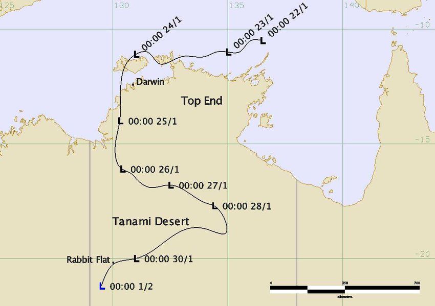
there have been recorded cases of storms re-intensifying              Interestingly, Evans et al. (2011) did speculate that “...
over land after initially weakening (Emanuel et al. 2008;          the development and organization of deep moist convection
Arndt et al. 2009; Brennan et al. 2009; Evans et al. 2011).        near the center of the vortex is necessary - and perhaps
Moreover, some tropical cyclones around the northern coast         sufficient - for vortex re-intensification to occur”. While
of Australia originate from tropical lows that first form over     they did not show details of the convection, they did show
land before moving over the sea and intensifying further           an increase in “the temporally and area-integrated vertical
(e.g. Tory et al. 2007; Smith et al. 2015a). Even if they          mass flux” within a column 100 × 100 km2 centered on the
remain over land, tropical lows often give rise to prodigious      simulated vortex in all their simulations (their Fig. 18).
amounts of rainfall and can cause serious flooding over
a wide area. Since comparatively little has been known                During the last decade, advances in understanding
in detail about their formation pathways and structure,            maritime tropical cyclogenesis have emerged from seminal
these lows pose significant challenges to forecasters. One         studies by Hendricks et al. (2004), Montgomery et al.
question is to what extent the formation, structure and            (2006), and Dunkerton et al. (2009). A review of this and
intensification of these lows over land are similar to those       other research on the topic was given by Montgomery and
of tropical cyclones over sea?                                     Smith (2011). Hendricks et al. (2004) and Montgomery
   An early pioneering and insightful analysis of tropical         et al. (2006) drew attention to the important role of rotating
cyclogenesis in the Australian region is provided by               deep convection during genesis, while Dunkerton et al.
McBride and Keenan (1982) and since then there have been           (2009) examined the nurturing role of a tropical wave
one or two early case studies of lows that initially formed        and presented a new framework for understanding how
over land (Foster and Lyons 1984; Davidson and Holland             such hybrid wave-vortex structures develop into tropical
1987).                                                             depressions. Rotating deep convection has been shown
   Emanuel et al. (2008) pointed out that even in the absence      to be a feature also of the subsequent intensification of
of appreciable extratropical interactions, and although the        tropical cyclones (Nguyen et al. 2008; Montgomery et al.
underlying soil is desert sand, some cyclones making               2009; Smith et al. 2009; Bui et al. 2009; Fang and Zhang
landfall over northern Australia may re-intensify to the point     2010; Persing et al. 2013). In this paper we examine an
of reacquiring the classical inner-core structure of a cyclone,    alternative hypothesis to Emanuel et al. (2008): namely
including an eye. They presented a case study of such an           that the formation and intensification or re-intensification
event (Tropical Cyclone Abigail 2001). They hypothesized           of tropical lows over land in a monsoonal environment is a
that the intensification or re-intensification of these systems,   similar process to that which occurs over the sea and is not
which they christened “agukabams”, is made possible by             dependent on special properties of the soil.
large vertical heat fluxes from a deep layer of very hot,
sandy soil that has been wetted by the first rains of the             A relatively well observed example of a low that
approaching systems, significantly increasing its thermal          developed near the coast and intensified as it drifted
diffusivity. In support of this hypothesis, they presented         inland is the one that formed near the north coast of
results simulations with a simple axisymmetric tropical            Australia during the Tropical Warm Pool International
cyclone model coupled to a one-dimensional soil model.             Cloud Experiment (TWP-ICE) in January 2006 (May et al.
These axisymmetric simulations indicated that warm-core            2008). This low passed over Darwin, the focal point for
cyclones could intensify when the underlying soil is               the experiment, before moving inland and intensifying as
sufficiently warm and wet and are maintained by latent heat        it moved southwards over several days. In its early stages,
transfer from the soil. The simulations suggested also that        the low was well sampled by a network of radiosonde
when the storms are sufficiently isolated from their oceanic       soundings in the Darwin region, data which should have
source of moisture, the rainfall they produce is insufficient      benefited global analyses of the low at these stages.
to keep the soil wet enough to transfer significant quantities     However, the subsequent intensification took place over
of latent heat, and the storms then decay rapidly.                 a relatively data sparse region of the Northern Territory
   Evans et al. (2011) carried out numerical simulations           where reliance on analyses of the global models for storm
of Tropical Storm Erin (2007), which made landfall as a            behaviour is required. In this paper we present a series of
tropical depression from the Gulf of Mexico and underwent          numerical simulations of this low, which captured the inland
re-intensification as it moved northeastwards over the             intensification as seen in the European Centre for Medium
central United States (Arndt et al. (2009), Brennan et al.         Range Weather Forecasts analyses (ECMWF) for the event.
(2009)). They found that the Emanuel et al. (2008) along-          Analyses of these simulations indicate that, indeed, the
track tropical cyclone rainfall feedback mechanism to be of        intensification does conform with the new paradigm for the
minimal importance to the evolution of the vortex. They            intensification of maritime storms summarized recently by
concluded that “ ... the final intensity of the simulated          Montgomery and Smith (2014) and Smith and Montgomery
(and presumably observed) vortex appears to be closely             (2015b).
linked to the maintenance of boundary layer moisture over
preexisting near-climatological soil moisture content along           The remainder of the paper is structured as follows.
the track of the vortex and well above climatological soil         Section 2 gives an overview of the tropical low and
moisture content”. Citing Montgomery et al. (2009) they            section 3 gives a brief description of the numerical model.
noted that tropical cyclone development over water requires        Section 4 describes the vortex development in the numerical
only a modest elevation of surface latent heat fluxes beyond       simulations. Section 5 examines the basic dynamics of
those of nominal trade-wind values on the order of 150 W           vortex spin up in an axissymmetric framework. Section 6
m−2 : it does not require these fluxes to continue to increase     examines the reasons for the differences in behaviour for
with increasing wind speed (see also Montgomery et al.             all sensitivity simulations on the second day and section 7
2015), which would appear to be an essential feature of the        investigates aspects of the thermodynamic support for spin
axisymmetric model used by Emanuel et al. (2008).                  up. The conclusions are given in section 8.

          Copyright c 2015 Royal Meteorological Society                          Q. J. R. Meteorol. Soc. 5: 1–14 (2015)
                    Prepared using qjrms4.cls
Figure 2. Time series of the minimum sea-level pressure, Pmin , and
maximum horizontal total wind speed at the height of 850 mb, Vmax , of
NT2006 as seen in the ECWMF analyses.
Figure 1. Best-track position of NT2006 with place names mentioned in
the text. (Image courtesy of Ian Shepherd, Northern Territory Regional
Office, Australian Bureau of Meteorology) 3. The model configuration
The numerical experiments are performed using the
2. Overview of the tropical low Pennsylvania State University/National Center for Atmos-
pheric Research fifth-generation Mesoscale Model (MM5
The case chosen for investigation herein is an unnamed version 3.6.1). MM5 is a non-hydrostatic sigma-coordinate
low (subsequently referred to as “NT2006”) that formed model designed to simulate or predict mesoscale atmos-
off the north coast of the Northern Territory around 00:00 pheric circulations (Dudhia 1993; Grell et al. 1995). The
UTC∗ 22 Jan during the TWP-ICE. During the following model is configured here with two domains: a one-way
two days it moved westwards and strengthened into a nested outer domain of 9 km grid spacing, and a two-way
tropical storm, making landfall in the Darwin area around nested inner domain of 3 km grid spacing with the centre
18:00 UTC 24 Jan, before drifting down the western border located at 16◦ S,132.5◦E. The domains are rectangular and
of the Northern Territory. After landfall, the low moved have 201×203 and 493×505 grid points for the outer
southwards and weakened, but around 00:00 UTC 26 Jan, it domain and inner domain, respectively. There are 23 σ-
began to track southeastwards and re-intensified, achieving levels in the vertical direction† . Ten of these levels cover the
its maximum strength at 00:00 UTC 28 Jan. Thereafter it region from the surface to 850 mb to provide an adequate
gradually weakened over land and from 00:00 UTC 29 Jan it vertical resolution for representing the planetary boundary
began to move slowly southwestwards. The low initiated an layer. The pressure of the model top, ptop , is set to 100 mb.
active monsoon onset over the Top End and brought heavy
The planetary boundary-layer is modelled using the
rainfall to many parts of the western Northern Territory,
Hong-Pan scheme (Hong and Pan 1996) and deep moist
including some areas of the Tanami Desert, which exceeded
convection is represented explicitly using a simple-ice
their annual average rainfall in a few days. There was heavy
scheme (Dudhia 1993). No cumulus parameterization is
rainfall in the Darwin region also, with many 24 hour
used. The cloud-radiation scheme is used as a radiative
totals exceeding 100 mm. Figure 1 shows the best-track
cooling scheme and the five-layer soil model is used as a
position of NT2006 from 00:00 UTC 22 Jan to 00:00 UTC
surface scheme.
1 February. The only observational data on the intensity of
the low came from the Bureau of Meteorology’s automatic In MM5, the surface evaporation depends on a parameter
weather station at Rabbit Flat, where near surface sustained called moisture availability (Ma )‡ which is used to
winds of 15 m s−1 and 16 m s−1 were recorded at 08:00 represent the effects of stomatal resistance, aerodynamic
UTC and 11:00 UTC on 31 Jan, respectively. resistance and soil moisture (Eckel 2002). In the control
experiment, the initial value of Ma in a certain model grid
Figure 2 shows the time series of the minimum sea-level
pressure, Pmin , and maximum total (horizontal) wind speed box is obtained from a look-up table based on the land type
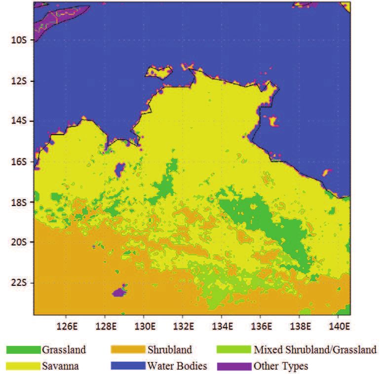
at 850 mb, Vmax , of NT2006, obtained from the ECMWF and season (Dudhia et al. 2005, Table 4.2c). The main land
analyses. Based on these time series, we can identify three types for the present MM5 simulation are savanna, water
stages of evolution: (1) the first stage is from 18:00 UTC bodies and shrub land (Figure 3), whose default Ma values
24 Jan to 00:00 UTC 26 Jan during which time the vortex are 15%, 10% and 100% in the northern summer.
intensity at 850 mb has a time mean value of about 19 m The initial data and boundary conditions are provided by
s−1 and the time mean value of Pmin is about 999 mb; the ECMWF analyses.
(2) the second stage is from 00:00 UTC 26 Jan to 00:00
† The
UTC 28 Jan during which Pmin begins to fall steadily and values of σ are: 0.9975, 0.9925, 0.985, 0.975, 0.965, 0.955, 0.94,
Vmax increases to about 31 m s−1 ; (3) the third stage is from 0.92, 0.9, 0.87, 0.83, 0.79, 0.75, 0.71, 0.67, 0.63, 0.59, 0.55, 0.51, 0.47,
0.375, 0.225 and 0.075
00:00 UTC 28 Jan to 06:00 UTC 29 Jan during which Pmin ‡ Specifically, the formula for the moisture availability is M =
a
steadily increases and Vmax steadily decreases. It is during E/[CE V1 ρ(q0∗ − q1 )], where E is the surface evaporation rate [unit kg
the second stage that NT2006 re-intensified over land. This m−2 s−1 ], CE is the moisture exchange coefficient, V1 is the wind speed
period will be the focus of the present paper. [unit m s−1 ] at a height h1 [unit m] at which the wind speed and moisture
are measured, ρ is the air surface density [unit kg m−3 ], q0∗ is the saturation
mixing ratio at the surface and q1 is the mixing ratio at height h1 , typically
∗ Universal Time Coordinated. 2 m, the lowest model level (Eckel 2002).
Copyright c 2015 Royal Meteorological Society Q. J. R. Meteorol. Soc. 5: 1–14 (2015)
Prepared using qjrms4.clsrelative to the vortex centre, defined here as the location of
the minimum sea-level pressure¶ within a radius of 150 km.
The MM5 calculations begins at 00:00 UTC 26 Jan,
30 hours after the storm made landfall. On 25 Jan, the
storm intensity in the ECMWF analysis was quasi-steady
with Pmin increasing slightly from 999 mb to 1000.6 mb,
V Tmax lying around 19 m s−1 and Vmax around 9 m s−1 .
(a)
Figure 3. MM5 land use for the outer domain
3.1. Sensitivity experiments
As suggested by previous studies, it is reasonable to
expect that the surface evaporation rate would be an
important element in the intensification of tropical lows
over land since, in order to maintain deep convection,
there has to be a mechanism to replenish the moisture
that convection consumes. However, over land, the surface
evaporation depends on the surface moisture, a quantity (b)
that is not routinely measured. For this reason, in the
calculations to be described, we examine the sensitivity
of the calculations to the initial moisture availability.
Altogether, seven calculations are presented: a control
experiment and six other experiments, which are detailed
in Table I. In all experiments except C6, the bucket soil
moisture scheme§ is used so that Ma is allowed to vary with
space and time in response to rainfall and evaporation rates.
In experiment C6, Ma is held fixed: it is not allowed to vary
with time in response to rainfall and evaporation rate.
The MM5 integrations all commence at 00:00 UTC 26
Jan and run for 48 h. Data are examined at time intervals of
5 min. The results are presented in the next section. (c)
4. The numerical simulations Figure 4. Vortex development in both ECMWF analyses and MM5
simulations C0-C6. Time series of: (a) minimum sea-level pressure Pmin ;
(b) maximum total wind speed V Tmax and (c) maximum azimuthally-
4.1. Overview of vortex development averaged tangential wind component Vmax at 900mb.
We present first an overview of the storm’s intensification After initialization at 00:00 UTC 26 Jan, the vortex in
after landfall (stage II) in the control simulation and in all the MM5 calculations undergoes an adjustment phase
the additional sensitivity simulations. Figure 4a shows in which Vmax decays slightly during the first hour, before
time series of the minimum sea-level pressure Pmin for intensifying rapidly over the next two hours and then
both ECMWF analyses and MM5 simulations C0-C6. decaying over a further six hours to a value close to that
Figures 4b and 4c show the maximum total wind speed in the ECMWF analysis, about 11 m s−1 . Following this
V Tmax and maximum azimuthally-averaged tangential adjustment phase, Vmax remains approximately steady in
wind component Vmax at 900 mb (approximately 870 m
high) respectively. The azimuthal average is calculated
¶ An alternative definition of the vortex centre might be the location of
minimum total wind speed at some low level and within some radius of
§ In the MM5 model, the bucket soil moisture scheme keeps a budget of the minimum sea-level pressure centre. However, it was found that the
soil moisture allowing moisture availability to vary with time, particularly locations of the minimum sea-level pressure and minimum absolute wind
in response to rainfall and evaporation rates. (Dudhia et al. 2005, pp8-15) at 900 mb are mostly within 10 km of each other
Copyright c 2015 Royal Meteorological Society Q. J. R. Meteorol. Soc. 5: 1–14 (2015)
Prepared using qjrms4.clsSymbol Description
C0 Control experiment using the default Ma values in summer
C1 As C0, except that the initial value of Ma is decreased by 20%
C2 As C0, except that the initial value of Ma is decreased by 10%
C3 As C0, except that the initial value of Ma is increased by 10%
C4 As C0, except that the initial value of Ma is increased by 20%
C5 As C0, except that the initial value of Ma is increased by 50%
C6 As C0, except that Ma is not allowed to vary with time in response to rainfall and evaporation rates
Table I. Control and six sensitivity simulations
both the MM5 model and in the ECMWF analyses for a the centre of circulation, a feature that is particularly
period of about 12 h before increasing gradually during conducive to vortex spin up by the conventional spin
27 Jan to reach about 15 m s−1 . The initial decay is up mechanism as discussed in the next section. The
not seen in the V Tmax curves, which are indicative of updraught cores are approximately colocated with regions
local rather than azimuthally-averaged conditions. After the of significantly enhanced vertical vorticity indicative of
initial adjustment phase, the agreement of the Vmax values the stretching of system-scale cyclonic vorticity by the
between the MM5 simulations and the ECMWF analyses updraughts (Hendricks et al. 2004; Montgomery et al. 2006;
is remarkably good. As would be expected, the agreement Kilroy and Smith 2013; Kilroy et al. 2014; Kilroy and Smith
is not so good when judged in terms of V Tmax , a result 2015). Hendricks et al. (2004) referred to these vortical
that is expected because of the higher horizontal resolution updraughts as “Vortical Hot Towers”.
of the MM5 calculations. The significantly higher values of Three hours later, at 06:00 UTC (15:30 CSTk ), deep
V Tmax in the MM5 calculations are consistent with the idea convection has collapsed within 50 km radius of the
that the higher resolution enables convective features to be circulation centre (Fig. 5c) although a region of enhanced
better represented and less smeared out than in the ECMWF relative vorticity remains around this centre (Fig. 5d). Soon
analyses. The grid spacing in ECMWF analyses is 0.125o after 08:00 UTC 27 Jan, the vortex undergoes two brief
(approximately 13 km) while in the MM5 model it is only 3 periods of intensification each lasting 1-2 hours (see blue
km for the inner domain. curve in Fig. 4c). As on the previous day, the existence
A significant finding is that there is no systematic of these periods coincides with the reappearance of deep
difference in the behaviour of V Tmax and Vmax between convective cells near the centre of circulation as exemplified
experiments C0 and C6, indicating that the along-track by the vertical motion field at 08:00 UTC shown in Fig.
rainfall has a minimal positive impact in terms of 5e. The two cells closest to the storm centre of circulation
vortex intensity. This result is presumably because the are accompanied by regions of enhanced vertical vorticity
rainfall across the vortex is patchy and doesn’t contribute as seen in Fig. 5f. These cells of deep convection do not
appreciably to surface moisture fluxes (see section 7). The survive over a diurnal cycle: indeed by 18:00 UTC 27 Jan
finding is in line with that of Evans et al. (2011) for Tropical (03:30 CST 28 Jan), when the vortex intensity has reached
Storm Erin (2007), but does not support the hypothesis a local maximum (Vmax ≈ 15 m s−1 ), there are no strong
of Emanuel et al. (2008), who suggest that the along- updraughts within a radius of some 90 km of the circulation
track rainfall is a significant factor in the overland re- centre. Six hours after this time the vortex begins a period
intensification of tropical cyclones over Australia. There of decay.
is little sensitivity of the V Tmax and Vmax values to the
initial value of Ma in the MM5 simulations on the first
day of integration, but the differences become larger (by 5. Dynamics of spin up
10% to 30%) on the second day. These differences may
be attributed to a stochastic element in the patterns of deep The spin up described in the previous subsection involves
convection as examined later in section 6. In general, the dynamical processes that are intrinsically asymmetric,
values of Pmin and Vmax for all MM5 simulations fit those although one can examine the dynamics of spin up from
in the ECMWF analyses well. an axisymmetric perspective by azimuthally averaging the
flow fields. In this perspective, departures from axial
4.2. Evolution of vertical velocity and relative vorticity symmetry in the mean momentum equations appear as
The left panels of Fig. 5 show patterns of the vertical “eddy terms” (Persing et al. 2013; Smith et al. 2015b).
velocity at 500 mb in the control experiment C0 at In this section we examine the basic dynamics of vortex
selected times. The right panels show the corresponding spin up in an axisymmetric framework and in section 7 we
patterns of the vertical component of relative vorticity at investigate aspects of the thermodynamic support for spin
850 mb with the storm-relative wind vectors at this level up. The primary focus here will be on the tangential wind
superimposed. The system translation velocity is based on component, v, as well as the surfaces of absolute angular
the movement of the vortex centre as defined in section momentum, M , henceforth referred to as the M -surfaces,
4.1. The top two panels show the situation at 03:00 UTC which are derived from this component. The quantity, M is
26 Jan during the initial period of rapid intensification. defined as
At this time, deep convection is evident in the pattern 1
M = r < v > + f r2 , (1)
of vertical velocity which has several strong irregularly- 2
spaced updraught cores with vertical velocities up to 11
m s−1 . Significantly, one updraught complex straddles k Central Standard Time = UTC + 9h 30 min
Copyright c 2015 Royal Meteorological Society Q. J. R. Meteorol. Soc. 5: 1–14 (2015)
Prepared using qjrms4.cls(a) (b)
(c) (d)
(e) (f)
(g) (h)
Figure 5. Vertical velocity at 500 mb (left panels) and the relative vertical vorticity at 850 mb with the storm-relative wind vectors superimposed (right
panels) at 03:00, 06:00 UTC 26 Jan and 08:00, 18:00 UTC 27 Jan in the control experiment C0. Contour interval for vertical velocity: thick curves 2.0
ms−1 and thin curves 0.4 m s−1 with highest absolute value 1.0 m s−1 . Contour interval for relative vorticity: thick curves 10×10−4 s−1 and thin
curves 4×10⁻⁴ s−1 with highest absolute value 6×10⁻⁴ s−1 . Cyclonic (negative) values are solid curves in red and anticyclonic (positive) values are
dashed curves in blue.
where r is the radius from the vortex centre, < v > is the Inspection of Fig. 5 suggests that the < v > and M -
azimuthally-averaged tangential wind speed, and f is the fields may have a higher degree of axial symmetry than,
Coriolis parameter, assumed to be a constant.
Copyright c 2015 Royal Meteorological Society Q. J. R. Meteorol. Soc. 5: 1–14 (2015)
Prepared using qjrms4.clsFigure 6. Radius-height cross-section of isotachs of azimuthally-averaged tangential wind at (a) 00:00, (b) 03:00, (c) 06:00 UTC 26 Jan and (d) 08:00,
(e) 18:00 UTC 27 Jan in the control experiment. Contour interval 2 m s−1 . Cyclonic (negative) values are solid curves and anticyclonic (positive) values
are dashed curves. The X symbol marks the position of the maximum azimuthally-averaged tangential wind.
for example, the vertical velocity and relative vorticity. We In fact, Fig. 4 shows that the intensity of the vortex is
show also the azimuthally-averaged radial wind component, on the decline at this time, which is near the end of the
but caution that this may be more prone to error than initial adjustment period. This decline continues for about
the tangential component because any error in the centre another three hours after which the intensity begins to
finding procedure can lead to aliasing of the tangential wind slowly increase. Nevertheless, at 08:00 UTC 27 Jan (Fig.
component into the radial component∗∗. 6d), the vortex is still a little weaker and shallower than at
Figure 6 shows radius-height plots of < v > in the 06:00 UTC on the previous day.
control experiment at the initial time and at same times The increase in intensity is most marked during the
as in Fig. 5. At the initial time, 00:00 UTC 26 Jan (Fig. following 10 hours, the maximum < v > increasing by
5a), there is a monotonic increase in < v > out to 150 km, about 4 m s−1 to 15.2 m s−1 (Fig. 6e). Even so, the
the maximum radius shown, and the maximum < v > (9 m maximum < v > is located at a radius of 100 km from the
s−1 ) occurs at about σ = 0.8 (on the order of 2 km height). storm centre at this time. It is noteworthy that this maximum
Three hours later, at 03:00 UTC (Fig. 5b), the winds at low occurs always at low levels with values of σ exceeding 0.8,
levels have increased with two prominent local maxima, corresponding with heights of approximately 2 km or less.
one at a radius of about 15 km and the other at a radius of Figure 7 shows radius-height plots of the azimuthally-
about 80 km. both being a little over 12 m s−1 . Inspection averaged radial velocity superimposed on the M -surfaces
of Fig. 5a suggests that the low-level spin up is associated at the same times as those in Fig. 6. Values of M less than
with the early development of deep convection near the 4×10⁵ m2 s−1 are highlighted in blue to represent some
circulation centre and that the local maximum of < v > is inner core region, and those larger than 1×10⁶ m2 s−1 are
associated with the convective cell at the axis. Three hours highlighted in red in Fig. 7 to represent some outer core
later, at 06:00 UTC (Fig. 6c), the vortex has strengthened in region.
depth, but the maximum < v > has increased only slightly. Prominent structural features are that, in the lower
troposphere, at least for values of σ exceeding 0.5, M
∗∗ An estimate of error in the radial wind due to error in the centre finding increases with radius at each level at each time, implying
has been carried out by moving the centre 15 km northward, southward, that the vortex is centrifugally (or inertially) stable (e.g.
eastward, and westward in the control experiment. It was found that the
time-averaged error in the radial wind within a radius of 15 km of the
Shapiro and Montgomery 1993; Franklin et al. 1993); and
centre can be as large as 90%, but the error falls rapidly to less than 25% that the M -surfaces slope inwards with decreasing radius
beyond this radius. within the boundary layer and outwards with radius aloft.
Copyright c 2015 Royal Meteorological Society Q. J. R. Meteorol. Soc. 5: 1–14 (2015)
Prepared using qjrms4.clsFigure 7. Radius-height cross-section showing contours of azimuthally-averaged radial velocity and the magnitude of the absolute angular momentum
at (a) 00:00, (b) 03:00, (c) 06:00 UTC 26 Jan and (e) 08:00, (f) 18:00 UTC 27 Jan in the control experiment. Contour interval for absolute angular
momentum: blue curves 1×10⁵ m2 s−1 with highest value 4×10⁵ m2 s−1 ; red curves 2×10⁵ m2 s−1 . Contour interval for radial velocity is 2 m
s−1 , positive values are solid curves and negative values are dashed curves. The X symbol markes the position of the maximum azimuthally-averaged
tangential wind.
These slopes give rise to a nose-like feature near the top of
the boundary layer. As explained in Smith et al. (2015b, see
their section 7.1), this structure of the M -surfaces may be
understood as follows. Above the boundary layer, < v > is
close to gradient wind balance and thermal wind balance.
Thus, because the tropical cyclone vortex is warm cored,
the M -surfaces lean outwards there. The inward-slope of
the M -surfaces near the surface is manifestation of the
reduction of < v > and hence M by the frictional torque
at the surface and the corresponding turbulent diffusion of
< v > to the surface. Figure 8. Time-height cross sections of the vertical mass flux per unit area
(Unit: 10−2 kg m−2 s−1 ) within a box 300 km × 300 km centred on the
The figure shows also that during periods of intensifica- location of the minimum sea-level pressure in the control experiment. Time
tion, the M -surfaces in the low to mid troposphere move zero corresponds to the start of the simulation at 00:00 UTC 26 Jan.
radially inwards so that the tangential winds are amplified
(because < v >= M/r − 12 f r). In the upper troposphere,
the M surfaces move radially outwards. As discussed in Figure 8 shows time-height cross sections of the vertical
section 4.2, the periods of intensification are associated with mass flux ρw, averaged over a square box 300 km × 300 km
the development of deep convection near the circulation centred on the location of the minimum sea-level pressure in
centre. The collective effects of this convection generate an the control experiment. Here, ρ is the density and w is the
overturning circulation with inflow in the lower troposphere vertical velocity. Notable features of the mass flux within
that converges the M -surfaces above the boundary layer, the box are two “bursts” centred at 03:00 UTC 26 Jan (3 h
where to a first approximation, M is materially conserved. in the figure) and 08:00 UTC 27 Jan (32 h in the figure).
In contrast, during the period of decay between 03:00 UTC Interestingly, the two bursts are each accompanied by an
and 06:00 UTC 26 Jan, the pattern of inflow and outflow increase of the maximum tangential wind speed (Fig. 4c).
are reversed, as is the radial movement of the angular These bursts are not obviously related to the diurnal cycle
momentum surfaces in the upper and lower troposphere. of convection over land.
Copyright c 2015 Royal Meteorological Society Q. J. R. Meteorol. Soc. 5: 1–14 (2015)
Prepared using qjrms4.clsFigure 9. Radius-height cross-section of the azimuthally-averaged
potential temperature anomaly from the areal mean (unit: K), time
averaged during the period of rapid intensification from 05:00 to 11:00
UTC 27 Jan in the control simulation.
Figure 10. Time series of the area-averaged vertical mass flux within a
radius of 30 km from the centre at 500 mb for all sensitivity simulations.
Time zero corresponds to the start of each simulation at 00:00 UTC 26 Jan.
The foregoing results are similar to those found for an
idealized tropical cyclone by Smith et al. (2009) and in
observations and simulations of a major hurricane (Evans
result of the convectively-induced inflow of air towards the
et al. 2011; Montgomery et al. 2014; Smith et al. 2015b),
circulation centre. If convection develops near the centre of
suggesting that the intensification mechanism of tropical
the circulation, the inflow it produces draws the M -surfaces
lows over land is similar to that of tropical cyclones. Perhaps
inwards and, since M is materially conserved there, the
the main difference is the much weaker radial inflow in the
tangential wind increases as described in section 5.
low studied here suggesting that the boundary layer control
on convection (Kilroy et al. 2016) is much less than in a Figure. 10 shows time series of the area-averaged vertical
tropical cyclone. mass flux (M F ) within a radius of 30 km from the
In contrast to the similarities with tropical cyclones centre at 500 mb for all sensitivity simulations. In each
over the sea, the azimuthally averaged thermal structure case, the variation of M F is, to some extent, similar
shown in Fig. 9 would appear to be somewhat different. to that of Vmax in Fig. 4c, supporting the idea that the
While the system is warm cored, the maximum potential occurrence of convection near the centre of the circulation
temperature anomaly is found in the lower troposphere is a key requirement for the spin up of the azimuthally-
rather than in the middle to upper troposphere as is usual averaged tangential winds. It may be significant that only
in tropical cyclones. It turns out, however, that because the experiments whose M F values become close or exceed
of weak vertical shear, the thermal anomaly in the mid 0.2 on 27 Jan undergo a burst of rapid intensification.
to upper troposphere (pressures 500 mb and lower) is The peak values of M F for C1 are up to 0.6 and 0.2 at
displaced by several tens of kilometres to the southwest approximately 05:30 and 15:00 on 27 Jan, respectively. It
relative to that at low levels and may be concealed by is at approximately the same time that Vmax shows sharp
the azimuthal averaging about a vertical axis. Even so, increases. Similarly, the curves for Vmax in experiments C2,
horizontal plots of potential temperature at each height (not C0 and C5 show sharp increases at approximately the same
shown) indicate that the maximum azimuthally-averaged time that their M F values are close to or greater than 0.2. In
potential temperature anomaly is still located in the lower contrast, in experiments C3 and C4, where the M F values
troposphere rather than mid or upper troposphere. This are much smaller than 0.2, Vmax does not show any burst of
feature is consistent with the fact that the vertical shear of rapid intensification.
the tangential wind is a maximum in the lower troposphere Figure 11 shows the vertical velocity at 500 mb
(Fig. 6). together with horizontal wind vectors at 850 mb at times
corresponding approximately with the brief times of rapid
6. Sensitivity simulations intensification in experiments C1, C2, C0 and C5 on 27 Jan
(panels a-d). This figure shows also two arbitrarily chosen
Referring back to Fig. 4, the sensitivity simulations in snapshots in experiments C3 and C4 (panels e-f) at the
which the initial moisture availability is varied indicated foregoing times. In experiments C1, C2, C0 and C5 there
little sensitivity of Pmin , V Tmax and Vmax on the first are convective updraughts at and near the circulation centre.
day of integration, but significant differences in behaviour For example, in experiments C1 and C2 at 06:00 UTC 27
emerge on the second day. The reasons for these differences Jan, there are updraughts within a radius of 10-20 km of
are examined now. the vortex centre with a maximum speeds of approximately
The curves for Vmax in experiments C1, C2, C0 and C5 7 m s−1 (Fig. 11a and Fig. 11b, respectively). In contrast,
show sharp increases at approximately 06:00, 06:00, 08:00 in experiment C4 (Fig. 11e) the strongest updraughts are
and 12:00 UTC 27 Jan, respectively (Fig. 4c), indicating a approximately 150 km to the northwest of the vortex centre,
brief period of rapid spin up near these times. In contrast, again with vertical velocity maxima of 7 m s−1 . There is
there are no such periods in the other two simulations just one updraught with a maximum velocity a little over 1
C3 and C4. The differences in behaviour between these m s−1 about 50 km west-southwest of the vortex centre.
two sets of simulations are a reflection of the stochastic At 08:00 UTC 27 Jan in experiment C0 (Fig. 11c), there
nature of deep convection and may be understood in is an updraught extending northwards from the centre and
terms of the classical mechanism for spin up (Ooyama another one extending 30 km to the southeast. These have
1969; see also Montgomery and Smith 2014). From an vertical velocities up to 5 m s−1 and 7 m s−1 , respectively.
azimuthally-averaged perspective, the spin up of the mean At the same time, in experiment C3, the nearest significant
tangential winds above the boundary layer occurs as a updraughts lie at a radius of about 40 km from the centre
Copyright c 2015 Royal Meteorological Society Q. J. R. Meteorol. Soc. 5: 1–14 (2015)
Prepared using qjrms4.cls(a) (b)
(c) (d)
(e) (f)
Figure 11. Vertical velocity at 500 mb together with wind vectors at 850 mb for (a) experiment C1, and (b) experiment C2 at 06:00 UTC 27 Jan; (c)
experiment C0 at 08:00 UTC 27 Jan; (d) experiment C5 at 12:00 UTC 27 Jan; (e) experiment C4 at 06:00 UTC 27 Jan; (f) experiment C3 at 08:00 UTC
27 Jan. Contour interval: thick curves 2.0 m s−1 and thin curves 0.4 m s−1 with highest absolute value 1.0 m s−1 . Positive values are solid curves in
red and negative values are dashed curves in blue.
(Fig. 11f). In experiment C5 at 12:00 UTC 27 Jan, there is In summary, the vortices in each of the experiments
−1 C1, C2, C0 and C5 have pulses of intensification that
an updraught with a velocity maximum of about 5 m s
are accompanied by strong convective updraughts near
located 10 km to the west of the vortex centre (Fig. 11d). the circulation centre. In experiments C3 and C4, there
Copyright c 2015 Royal Meteorological Society Q. J. R. Meteorol. Soc. 5: 1–14 (2015)
Prepared using qjrms4.clsare no such pulses and at no time do significant strength
updraughts develop near the vortex centre. These results
suggest the hypothesis that only the vortices that have deep
convection near their centre of circulation will undergo
pulses of rapid intensification. The results add further
support for the idea that a key requirement for the
intensification of storms in general is the occurrence of
deep convection near or at the existing centre of circulation.
This result accords with the findings of Smith et al. (2015a)
and Kilroy et al. (2015). The requirement transcends earlier
ideas invoking the increased efficiency of diabatic heating
in the high inertial stability region of the vortex core (e.g. (a)
Schubert and Hack 1982; Hack and Schubert 1986; Vigh
and Schubert 2009) for reasons articulated in a recent paper
by Smith and Montgomery (2015a). In essence, the most
effective spin up requires M -surfaces to be drawn inwards
to small radii. Geometrically speaking, convection located
at a given radius can only draw air inwards outside that
radius. Inside that radius, air will be drawn outwards. Thus,
inside the convection radius, M -surfaces will be drawn
outwards with a consequent spin down there. In spite of
the fact that the large inertial stability at small radii will
oppose the inward displacement of the M -surfaces, only
convection located near the circulation centre is able to
draw the M -surfaces inwards to small radii to spin up the (b)
tangential circulation above the frictional boundary layer as
Figure 12. Sources and sinks of moisture including the contributions by
discussed in section 5. Note, the inflow in the vortices under surface evaporation (E), precipitation (P) and the horizontal transport of
study here is sufficiently weak (Figure 7) that the boundary moisture (S) in Eq. (2) averaged over boxes: (a) 300 km × 300 km, (b) 600
layer control ideas discussed by Kilroy et al. (2016) are only km × 600 km centred on the location of the minimum sea-level pressure
minimally operative. in the control experiment. Shown also is the total precipitable water (TPW)
in kg m−2 . Time zero corresponds to the start of the simulation at 00:00
The significant differences in the patterns of vertical UTC 26 Jan.
velocity fields for the different sensitivity simulations
in Fig. 11 highlight the stochastic variability of deep
convection resulting from the differences in the initial
moisture availability and, as shown above, this variability
adds a stochastic element to the intensification process
itself, consistent with the results of Nguyen et al. (2008)
and Shin and Smith (2008).
7. Thermodynamic support for spin up
In the two previous sections we have presented evidence
in support of Evans et al. (2011)’s speculation noted in
the Introduction that the development and organization of
deep moist convection near the centre of the vortex is
necessary for vortex intensification to occur. The question
remains, however, where does the moisture come from to Figure 13. Time series of the area-averaged surface latent heat flux within
support sustained deep convection near the vortex centre a radius of 150 km from the centre in the control experiment. Time zero
over land? In particular, how important are surface moisture corresponds to the start of the simulation at 00:00 UTC 26 Jan.
fluxes compared to the horizontal advection of moisture in
maintaining deep convection? In a model simulation such
as ours that captures the intensification of a low over land, and S is the rate of moisture convergence through the
it should be possible to address these questions by way of a sides of the column. Moisture convergence is calculated
moisture budget analysis of the model output. by vertically integrating the fluxes of moisture into a box
We examine now the importance of surface evaporation centred on the system. These three quantities are then
compared with the horizontal transport of moisture into the averaged over the area of the box to provide units of kg m−2
system. A simple moisture budget for a vertical column of h−1 .
unit horizontal cross-section is given by: Figure 12 shows time series of terms in the moisture
budget for the control simulation, C0, for two columnar
∂T P W regions extending to the model top. One column has a
= E − P + S, (2) horizontal cross section 300 km × 300 km square centred
∂t
on the vortex centre and the other has a 600 km × 600 km
where ∂T P W/∂t is the change in total precipitable water square cross section. The terms include: the contributions to
(T P W ) with time, E is the rate of evaporation of moisture the box-averaged moisture tendency by surface evaporation
from the surface, P is rate of moisture loss by precipitation (E), precipitation (P ), and the horizontal transport of
Copyright c 2015 Royal Meteorological Society Q. J. R. Meteorol. Soc. 5: 1–14 (2015)
Prepared using qjrms4.clsexperiment. The curve mimics closely the behaviour of the
curve for E in Fig. 12, but is multiplied by the coefficient
of latent heat to give units of W m−2 . Again the diurnal
signal is a prominent feature with peak values at about 03:00
UTC on the order of 300 W m−2 . However, the mean value
averaged over a day is appreciably smaller, 103 W m−2 , a
value close to that found by (Evans et al. 2011, p. 3860) for
large areas of Tropical Storm Erin. Despite the smallness of
(a) the surface moisture fluxes in the overall moisture budget,
one should not conclude that these fluxes are unimportant.
Figure 14a shows a radius-height cross section of
pseudo-equivalent potential temperature, θe , in the control
experiment, time averaged during the period of rapid
intensification from 05:00 to 11:00 UTC 27 Jan.
The Emanuel theory for vortex intensification predicts
substantially elevated values of θe in the vortex core (e.g.
Emanuel 1989). In the theory, these are tied to an increase
(b) in the surface enthalpy fluxes accompanying an increase
Figure 14. (a) Radius-height cross-section of the azimuthally-averaged
in the surface wind speed with decreasing radius. There
pseudo-equivalent potential temperature (unit: K), time averaged during are, indeed, elevated values of θe in a shallow layer
the period of rapid intensification from 05:00 to 11:00 UTC 27 Jan in the near the surface, but the corresponding (negative) radial
control experiment. (b) A similar cross-section for Expt. C6 during the gradient is weak in the middle troposphere, unlike that
same time period.
envisaged in the Emanuel theory for vortex intensification
in an axisymmetric model (see e.g. Fig. 9.15b in Holton
2004). However, the elevated values of θe near the surface
moisture through the sides of the column (i.e. S). Shown contribute to the conditional instability of air in the inner
also is the total precipitable water (T P W ) averaged over region of the vortex. The need for such elevated values of
the column. Figure 12 shows that, at most times, the flux θe for a tropical cyclone to intensify was first pointed out by
of moisture into the sides of these two columnar regions Malkus and Riehl (1960).
is approximately equal to the amount of moisture lost by Figure 14b shows a similar cross section of θe in
precipitation, while the contribution from the mean surface experiment C6 in which the coupling between rainfall and
evaporation is small in comparison. Notwithstanding the moisture availability is suppressed. Again, near-surface θe
fact that the budget does not close because water substance values are elevated near the vortex centre, but not so much
is not strictly a conserved quantity in MM5 (Braun 2006), a as in the control experiment. Thus, even in this case, surface
similar result has been found also for tropical cyclones (e.g. fluxes act to support local conditional instability near the
Kurihara 1975; Braun 2006; Trenberth et al. 2007). vortex centre.
Focussing first on the 300 km × 300 km square column In summary, we have shown that the horizontal transport
(Fig. 12a), there is a steady decline in mean T P W from of moisture into a mesoscale box following the low is
an initial value of 68 kg m−2 to about 62 kg m−2 essentially equal to the moisture lost by precipitation.
at the end of the 48 h simulation. These are relatively The contribution to the moisture budget by surface fluxes
large values, but typical of the Australian monsoon regime is small in comparison. Nevertheless, the small moisture
(see e.g. Kilroy et al. 2015). For comparison, observed fluxes play an important role in generating convective
values found in the “pouch” regions of pre-genesis Atlantic instability in a monsoon environment that already has
and Carribean wave disturbances during the PREDICT relatively high values of T P W so that deep convective
experiment (Montgomery et al. 2012) were generally bursts can continue to occur even when the system is located
around 60 kg m−2 near the sweet spot of the pouch far inland.
(values for Tropical Storm Gaston are shown in Figs. 2
and 3 of Smith and Montgomery (2010)). Mean values of 8. Conclusions
T P W in monsoonal flow conditions at Darwin are typically
about 57 kg m−2 (Črnivec and Smith 2016). There are We have analysed the intensification of tropical low over
large fluctuations in S and P during the early adjustment land in numerical simulations of an event that occurred over
period (the first 8 h of the simulation), but these have northern Australia in January 2006 during the TWP-ICE
a relatively small net effect on the mean T P W change. experiment. A control simulation together with a series of
After the adjustment phase, there are two broad peaks in five sensitivity simulations were discussed. The sensitivity
precipitation, one centred around 19:00 UTC 26 Jan and simulations were determined by varying the initial moisture
the other around 08:00 UTC 27 Jan. Not surprisingly, these availability from that in the control calculation, a procedure
peaks coincide approximately with similar peaks in the that adds, inter alia, a stochastic element to the development
vertical mass flux shown in Fig. 8, but they are not obviously and evolution of deep convection. In one further simulation,
related to peaks in E, which have a clear diurnal signal. the coupling between moisture availability and model-
A similar behaviour of terms in the moisture budget for produced precipitation was suppressed. The results of the
the 600 km × 600 km square column is seen in Fig. 12b, simulations were interpreted in terms of the classical
but the magnitude of the fluctuations is smaller, especially axisymmetric paradigm for tropical cyclone intensification
during the adjustment period. with recent modifications.
Figure 13 shows time series of latent heat flux averaged The spin up of the low over land is shown to be favoured
within a radius of 150 km from the centre in the control by the development of deep convection near the centre of
Copyright c 2015 Royal Meteorological Society Q. J. R. Meteorol. Soc. 5: 1–14 (2015)
Prepared using qjrms4.clsthe circulation, which is initially weak. This convection Eckel, T., 2002: Perturbing MM5 Moisture Availability for Ensemble
leads to an overturning (in, up and out) circulation that Forecasting. [Available online at http://www.atmos.
draws absolute angular momentum surfaces inwards in the washington.edu/˜ ens/ pdf/ATMS547_JUN2002.
teckel.pdf].
lower troposphere leading to spin up of the azimuthally-
Emanuel, K., J. Callaghan, and P. Otto, 2008: A hypothesis for the
averaged tangential winds above the boundary layer. In redevelopment of warm-core cyclones over northern Australia. Mon.
this respect, the intensification process is similar to that Wea. Rev., 136, 3863–3872.
for tropical cyclones over sea. The intensification takes Emanuel, K. A., 1989: The finite amplitude nature of tropical
place within a moist monsoonal environment, which is cyclogenesis. J. Atmos. Sci., 46, 3431–3456.
evidently sufficient to support sporadic deep convection Evans, C., R. S. Schumacher, and T. J. Galarneau, 2011: Sensitivity in
within the low’s circulation. A moisture budget for two the overland reintensification of Tropical Cyclone Erin (2007) to near
soil moisture characteristics. Mon. Wea. Rev., 139, 3848–3870.
mesoscale columns of air encompassing the low show that
Fang, J. and F. Zhang, 2010: Initial development and genesis of
the horizontal import of moisture is roughly equal to the Hurricane Dolly (2008). J. Atmos. Sci., 67, 655–672.
moisture lost by precipitation whereas surface moisture Foster, I. J. and T. J. Lyons, 1984: Tropical cyclogenesis: A comparative
fluxes make only a small contribution to the overall budget. study of two depressions in the northwest of Australia. Quart. Journ.
Nevertheless, enhanced surface moisture fluxes near the Roy. Meteor. Soc., 110, 105–119.
circulation centre play an important role in supporting deep Franklin, J. L., S. J. Lord, S. E. Feuer, and F. D. Marks, 1993: The
convection and thereby the intensification process. The kinematic structure of Hurricane Gloria (1985) determined from
nested analyses of dropwindsonde and Doppler radar data. Mon. Wea.
evolution of the simulated low was largely unaffected when Rev., 121, 2433–2451.
the coupling between rainfall and moisture availability was Grell, G. A., J. Dudhia, and D. R. Stauffer, 1995: A description of the
suppressed. This is presumably the case because the rainfall fifth generation Penn State/NCAR mesoscale model (MM5). NCAR
is patchy across the vortex. Tech Note NCAR/TN-398+STR., 000, 138.
Hack, J. J. and W. H. Schubert, 1986: Nonlinear response of atmospheric
Acknowledgement vortices to heating by organized cumulus convection. J. Atmos. Sci.,
43, 1559–1573.
We are grateful to our colleague Gerard Kilroy, who gave Hendricks, E. A., M. T. Montgomery, and C. A. Davis, 2004: The role
of “vortical” hot towers in the formation of Tropical Cyclone Diana
generous help to the first author in setting up and running (1984). J. Atmos. Sci., 61, 1209–1232.
the MM5 model. We are grateful also to Hongyan Zhu and Holton, J. R., 2004: An Introduction to Dynamic Meteorology (4th Edn.).
an anonymous reviewer for their constructive comments Elsevier Academic Press., 535 pp.
on the original version of the submitted manuscript. ST Hong, S. Y. and H. L. Pan, 1996: Nonlocal boundary layer vertical
and MG gratefully acknowledge financial supports for this diffusion in a medium-range forecast model. Mon. Wea. Rev., 124,
research from the National Natural Science Foundation of 2322–2339.
China (91215302, 90715040), Key project of State Key Kilroy, G. and R. K. Smith, 2013: A numerical study of rotating
convection during tropical cyclogenesis. Quart. Journ. Roy. Meteor.
Lab. of Disaster Reduction in Civil Eng. (SLDRCE15-A- Soc., 139, 1255–1269.
04), RKS acknowledges support from the German Research — 2015: Tropical-cyclone convection: the effects of a vortex boundary
Council (Deutsche Forschungsgemeinschaft) under Grant layer wind profile on deep convection. Quart. Journ. Roy. Meteor.
number SM30-23 and the Office of Naval Research Global Soc., 141, in press.
under Grant No. N62909-15-1-N021. MTM acknowledges Kilroy, G., R. K. Smith, and M. T. Montgomery, 2016: Why do model
the support of NSF grant AGS-1313948, NOAA HFIP grant tropical cyclones grow progressively in size and decay in intensity
after reaching maturity? J. Atmos. Sci., 72, 487–503.
N0017315WR00048, NASA grant NNG11PK021 and the
Kilroy, G., R. K. Smith, M. T. Montgomery, B. Lynch, and C. Earl-Spurr,
U. S. Naval Postgraduate School.. 2015: A case study of a monsoon low that intensified over land as
seen in the ECMWF analyses. Quart. Journ. Roy. Meteor. Soc., 141,
References submitted.
Kilroy, G., R. K. Smith, and U. Wissmeier, 2014: Tropical cyclone
Arndt, D. S., J. B. Basara, R. A. McPherson, B. G. Illston, convection: the effects of ambient vertical and horizontal vorticity.
G. D. McManus, and D. B. Demkos, 2009: Observations of the Quart. Journ. Roy. Meteor. Soc., 140, 1756–1177.
reintensification of Tropical Storm Erin (2007). Bull. Amer. Meteor. Kurihara, Y., 1975: Budget analysis of a tropical cyclone simulated in
Soc., 99, 1079–1093, doi:10.1175/2009BAMS2644.1. an axisymmetric numerical model. J. Atmos. Sci., 32, 25–59.
Braun, S. A., 2006: High-resolution simulation of Hurricane Bonnie Malkus, J. and H. Riehl, 1960: On the dynamics and energy
(1968). Part II: Water budget. J. Atmos. Sci., 63, 43–64. transformations in a steady-state hurricane. Tellus, 12, 1–20.
Brennan, M. J., R. D. Knabb, M. Mainelle, and T. B. Kimberlain, 2009: May, P. T., C. Jakob, J. H. Mather, and G. Vaughan, 2008: Field research:
Atlantic hurricane season of 2007. Mon. Wea. Rev., 137, 4061–4088. Characterizing oceanic convective cloud systems. Bull. Amer. Meteor.
Bui, H. H., R. K. Smith, M. T. Montgomery, and J. Peng, 2009: Balanced Soc., 89, 153–155.
and unbalanced aspects of tropical-cyclone intensification. Quart. McBride, J. L. and T. D. Keenan, 1982: Climatology of tropical cyclone
Journ. Roy. Meteor. Soc., 135, 1715–1731. genesis in the Australian region. J. Clim., 2, 13–33.
Davidson, N. E. and G. H. Holland, 1987: A diagnostic analysis of two Montgomery, M. T., C. Davis, T. Dunkerton, Z. Wang, C. Velden,
intense monsoon depressions over Australia. Mon. Wea. Rev., 115, R. Torn, S. Majumdar, F. Zhang, R. K. Smith, L. Bosart, M. M.
380–392. Bell, J. S. Haase, A. Heymsfield, J. Jensen, T. Campos, and M. A.
Dudhia, J., 1993: A non-hydrostatic version of the Penn State/NCAR Boothe, 2012: The Pre-Depression investigation of cloud systems in
mesoscale model: Validation tests and simulation of an Atlantic the tropics (predict) experiment: Scientific basis, new analysis tools,
cyclone and cold front. Mon. Wea. Rev., 121, 1493–1513. and some first results. Bull. Amer. Meteor. Soc., 93, 153–172.
Dudhia, J., D. Gill, K. Manning, W. Wang, and C. Bruyere, 2005: Montgomery, M. T., S. V. Nguyen, R. K. Smith, and J. Persing, 2009: Do
PSU/NCAR Mesoscale Modeling System Tutorial Class Notes tropical cyclones intensify by WISHE? Quart. Journ. Roy. Meteor.
and User’s Guide: MM5 Modeling System Version 3. [Available Soc., 135, 1697–1714.
online at http://www2.mmm.ucar.edu/mm5/documents/ Montgomery, M. T., M. E. Nichols, T. A. Cram, and A. B. Saunders,
tutorial-v3-notes.html]. 2006: A vortical hot tower route to tropical cyclogenesis. J. Atmos.
Dunkerton, T. J., M. T. Montgomery, and Z. Wang, 2009: Tropical Sci., 63, 355–386.
cyclogenesis in a tropical wave critical layer: easterly waves. Atmos.
Chem. Phys., 9, 5587–5646.
Copyright c 2015 Royal Meteorological Society Q. J. R. Meteorol. Soc. 5: 1–14 (2015)
Prepared using qjrms4.clsYou can also read