NOAA Technical Report NOS NGS 64 - Blueprint for 2022, Part 2: Geopotential Coordinates

NOAA Technical Report NOS NGS 64

Blueprint for 2022, Part 2: Geopotential Coordinates

 November 13, 2017

 1

Versions
Date Changes
November 13, 2017 Original Release

 2

Acknowledgements
A work of this magnitude requires the input of many people. The contents of this document
grew out of a long list of scientific meetings inside NGS, beginning in 2014, and grew in scope
and frequency through 2015 and 2016. Many scientists inside NGS, and eventually outside of
NGS, contributed to the conversations, which ultimately led to this document. Recognition and
thanks for their contributions should go to the following individuals (in alphabetical order):

 Kevin Ahlgren, Dana Caccamise, Vicki Childers, Theresa Damiani, Michael Dennis,
 Joe Evjen, Steve Hilla, Simon Holmes, Jianliang Huang (GSC), Nic Kinsman, Xiaopeng Li,
 Dennis Milbert, Dan Roman, Brian Shaw, Dru Smith, Derek vanWestrum,
 Marc Véronneau (GSC), Yan Wang, Stephen White, Daniel Winester, Monica Youngman,
 Dave Zenk

 3

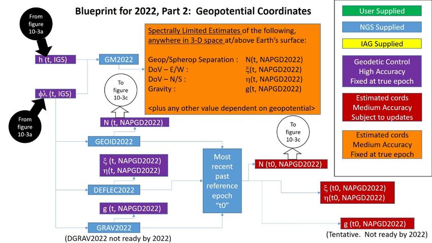
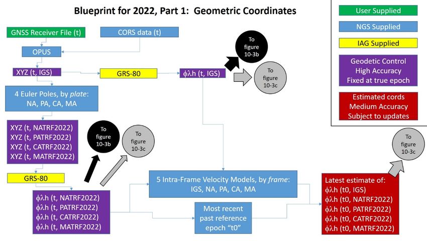
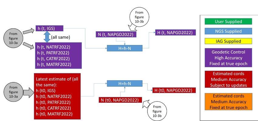
Executive Summary
 NOAA Technical Report NOS NGS 64
 Blueprint for 2022, Part 2: Geopotential Coordinates
In 2022, the entire National Spatial Reference System (NSRS) will be modernized. This
document addresses the geopotential aspects of the NSRS, including every vertical datum, the
geoid, gravity, deflections of the vertical, and other quantities related to Earth’s gravity field.
Every one of these related, yet semi-independent sources of information will be replaced with
an internally consistent geopotential datum called the North American-Pacific Geopotential
Datum of 2022 (NAPGD2022). Within NAPGD2022 four primary, interrelated time-dependent
products will exist:
 • A global model of Earth’s geopotential field (GM2022)
 • Regional gridded geoid undulation models (GEOID2022)
 • Regional gridded deflection of the vertical models (DEFLEC2022)
 • Regional gridded surface gravity models (GRAV2022)

The three regions for the gridded models will be North America (covering CONUS, Alaska,
Hawaii, the Caribbean, Canada, Mexico, Central America, and Greenland), American Samoa,
and Guam/Commonwealth of Northern Mariana Islands (CNMI).
NAPGD2022 will be built upon the IGS frame, as only minor (entirely horizontal) differences will
exist between the IGS frame and the four new terrestrial reference frames developed as part of
the NSRS in 2022 (see NGS, 2017). Since these differences will be relatively small horizontal
displacements (mainly due to Euler pole rotations), NAPGD2022 will operate equally well in any
of four new frames.
Orthometric heights in NAPGD2022 will be defined through ellipsoid heights and GEOID2022.
This means NAPGD2022 orthometric heights will primarily be accessed through Global
Navigation Satellite System (GNSS) technology. GEOID2022 will be defined in a manner that
best fits global mean sea level at the epoch of NAPGD2022. When global sea level changes by a
threshold level of 20 centimeters, a new geoid model, and thus geopotential datum, will be
released. Until then, updates to any component of NAPGD2022 will result in updating all
components of NAPGD2022 using sequential version numbering.
Leveling in NAPGD2022 will retain its current role of providing high-accuracy local differential
orthometric heights. The determination of absolute heights, however, which will provide the
context of local differential heights, will reside in the GNSS domain (i.e., will be based on IGS
ellipsoid heights).
Find this entire report here:
https://geodesy.noaa.gov/PUBS_LIB/NOAA_TR_NOS_NGS_0064.pdf

 4

Blueprint for 2022: Part 2, Geopotential Coordinates
The red text in the first three sections of this report is repeated verbatim from NOAA Technical Report
NOS NGS 62 (Blueprint for 2022, Part 1: Geometric Coordinates). The critical nature of this text to both
Geometric and Geopotential coordinates, as well as the need for consistency between the documents, is
the principal reason for this duplication.

Additionally, due to the large number of similar acronyms found throughout this document, a reference
glossary and list of abbreviations is provided at the end of this report.

1 Purpose

The intent of this document is to provide to the public the current status of plans by the National
Geodetic Survey (NGS) to modernize the National Spatial Reference System (NSRS) in 2022. This
particular document covers the Geopotential component; that is, the definition and determination of
orthometric heights, geoid undulations, 1 gravity, deflections of the vertical, dynamic heights, and any
other quantity directly related to the geopotential field of the Earth. Many abbreviations and
terminology specific to the new geopotential datum are used in this document. As a convenience to the
reader they are defined in the glossary at the end of the document.

This document does not attempt to be comprehensive, but it is being released with the express intent of
stating what is currently known, while leaving some items “to be determined” (TBD). As feedback is
collected about this document, further refinements to this blueprint will be made. It is expected that
updated releases of the blueprint will occur both before 2022 and shortly thereafter as more details
become codified.

Therefore, a word of caution is appropriate: Many portions of this document are purposefully vague.
NGS requests and welcomes feedback from the user community, particularly on those aspects, which
still have vague, TBD information.

2 Introduction

The mission of the National Geodetic Survey (NGS) is to define, maintain and provide access to the
National Spatial Reference System (NSRS), to meet our nation’s economic, social, and environmental
needs. The NSRS is defined by the Office of Management and Budget’s (OMB) circular A-16
(Coordination of Geographic Information and Related Spatial Data Activities) as “the fundamental
geodetic control for the United States” and is required to be used by all federal government agencies
creating geographic information within the United States.

1
 The terms “geoid undulation,” “geoid height,” and “geoid separation” have been used in a variety of sources
throughout the years, all with the same meaning: The distance, measured relative to a reference ellipsoid, along
the ellipsoidal normal, positive outward, to the geoid. This document will use the term “geoid undulation”
exclusively for this quantity.

 5

In order to keep up with changing technology and improved accuracy, NGS has planned for a
modernization of the NSRS by 2022. In order that this modernization maintains the usefulness of the
NSRS, the function of geodetic control should be clearly articulated first.

3 Geodetic Control

According to OMB A-16, “geodetic control provides a common reference system for establishing
coordinates for all geographic data.” That is, geodetic control is some system which allows users to
determine the latitude, longitude, height, gravity or other coordinate at points in their geographic
dataset in such a way that these coordinates are consistent with similarly derived coordinates prepared
by other users using other datasets, but using the same geodetic control. Therefore, geodetic control
must be more accurate than any map or other data set built upon it. There is no unanimous definition
of threshold values that define “geodetic accuracy” or “mapping accuracy”; this is especially true
considering (for example) that the state-of-the-art positioning accuracy was about 1 meter just a few
decades ago, but now it is in the centimeter and even millimeter range. Therefore, while terms like
“geodetic accuracy” or “mapping accuracy” (or “geodetic or mapping ‘quality’”) may be used in this
document, they should be taken relative to one another, rather than in an absolute sense. Geodetic
accuracy should be considered state-of-the art positioning accuracy, while mapping accuracy is anything
less accurate than that, but still capable of providing useful information in many map applications or
other geospatial products.

Unfortunately missing from this functional statement is the reality that geodetic control points (and
their respective coordinates) can, and do, move over time. A significant portion of this blueprint will be
dedicated to addressing why this is true and what can be done about it.

In order to fulfill its function, classical geodetic control was usually a network of metal disks or rods
affixed to the surface of the Earth with some associated coordinates such as latitude, longitude, height
or gravity, and where such coordinates are mutually consistent within the network. Such points served
as “starting points” for the users of geodetic control to begin their own surveys and thus create their
own maps or other geographic datasets. By requiring all federal creators of geographic data to use the
same geodetic control network (the NSRS), all geographic data in the USA created at the federal level
should therefore be mutually consistent.

As technology has progressed, our ability to establish accurate positions has outpaced the accuracy of
our underlying geodetic control. Coordinates do change over time due to a variety of factors operating
over different spatial and temporal scales. In general, these scales were either spatially small or
temporally very long, and were of a magnitude smaller than the accuracy of the surveys which created
the coordinates. For example, on a typical engineering timescale, coordinate drift is typically less than
the aforementioned 1 meter state-of-the-art absolute accuracy of the mid-late 20th century. Therefore,
it was possible for geodetic control to function for decades with the assumption of “fixed” coordinates,
only occasionally getting updated in certain locations when movement, exceeding the accuracy of
existing surveys, was finally detected.

Many surveyors still have equipment, software and other tools which presume that geodetic control
remains “fixed” (constant) in time. This simplifies project planning and computations significantly and

 6

also align with the majority of geodetic control services historically provided by NGS within the NSRS.
But it ignores the true nature of the Earth by oversimplifying geospatial data collected at different points
in time and limiting the ability to combine datasets that cover very large geographic areas. Although this
situation is changing, not all users of geodetic control can readily adapt to a system where coordinates
change in time. As such, some compromise is necessary for practical purposes when modernizing the
NSRS.

It should be pointed out that “horizontal control” (a point that provides latitude and longitude) was
generally considered stable and reliable for decades, except in locations of known significant crustal
deformation, such as in southern California. It was not until the advent of space geodesy that issues
such as the rotation of the entire tectonic plate (at centimeters per year) were seen to be affecting such
control. Contrast that with “vertical control” (points providing orthometric heights, or “elevations”).
Such control was well known from early on to be susceptible to (vertical) motions. Vertical motion,
relative to neighboring points, was occasionally detected upon re-surveying. Methods for avoiding such
movement have been used for decades, such as setting the points into bedrock or structures with deep
foundations, or driving rods to refusal. The success of such methods is not entirely clear, as no
comprehensive re-evaluation of the level network in the United States has ever been accomplished.
However, even methods which affix a mark to bedrock will be susceptible to vertical motion if the
bedrock itself is moving, such as is the case for the entire northeast portion of the North American
continent, due to the Glacial Isostatic Adjustment (GIA) centered around Hudson Bay. But as a
significant portion of the passive control points in the United States are poured-in-place concrete
markers set into the soil, any subsidence or uplift affecting the soil layer will also impact the elevation of
these points.

The purpose of geodetic control is to provide starting points by which geospatial users may define
positions with the consistency and reliability of the National Spatial Reference System. Such starting
points should have known coordinates at the epoch when the geospatial professionals are using that
control. If those coordinates have changed over time, then it would be convenient if some component
of the geodetic control should allow for comparison of previously determined geospatial coordinates at
different epochs.

4 The role of leveling in defining continent-wide geodetic control

Using passive vertical control as a method for defining and accessing a vertical datum suffered not only
from the vertical motion of marks (see above), but also from the methodology used to determine the
heights on those marks: geodetic leveling. Until the advent of space geodetic positioning techniques
(GNSS) and also the advent of accurate modeling of the geoid, the only reliable way to determine
heights with geodetic accuracy was to use geodetic leveling, a line-of-sight method generally restricted
to approximately 50- to 100-meter sight lengths, depending on the accuracy goal. Additionally, some
absolute starting height (or heights) had to be predetermined by other methods (e.g. choosing Local
Mean Sea Level [LMSL] at a convenient tide gauge on an island or in remote parts of the country, or
forcing groups of tide gauges to average their LMSL values to zero), as geodetic leveling is a purely
relative height-determining process.

 7

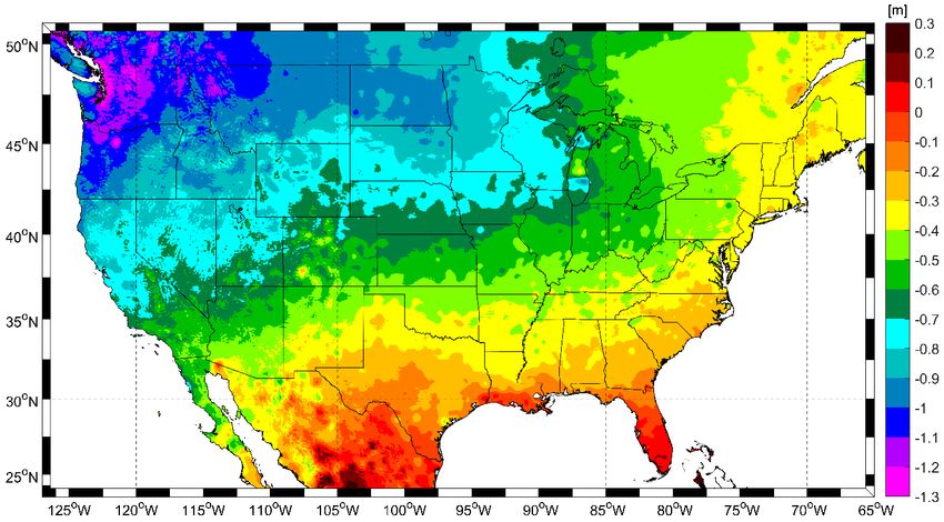
Leveling is well known to yield very accurate differential heights 2 in local areas (sub-millimeter over a
kilometer). However, it was used to determine continental-scale vertical datums, such as the National
Geodetic Vertical Datum of 1929 (NGVD 29) and the North American Vertical Datum of 1988 (NAVD 88).
The build-up of errors using such a localized tool in a project of continental size was difficult to gauge,
and this was especially true for NAVD 88, which held a single point (Father Point, in Rimouski, Canada)
as fixed (Zilkoski et al, 1992.) Around 2005 or thereabouts, it finally became possible to independently
evaluate the absolute accuracy of NAVD 88 heights. By that time GNSS-derived ellipsoid heights were
accurate to centimeters, and the Gravity Recovery and Climate Experiment (GRACE) mission yielded
a continental scale geoid model accurate to 1 centimeter over wavelengths longer than approximately
200 kilometers. These could be combined in the classic equation relating orthometric heights (H),
ellipsoid heights (h) and geoid undulations (N):

 ≈ ℎ − (1)

Equation 1 is approximate, because H is measured along a curving plumb line, while h and N are on
straight lines normal to the reference ellipsoid. However, the error in the approximation never exceeds
1 millimeter anywhere on Earth (Jekeli, 2000, equation 34).

Once N was determined from GRACE and h from GNSS, the GRACE/GNSS orthometric heights could be
checked against the leveling-derived NAVD 88 orthometric heights. This revealed that NAVD 88 heights
were, on average, biased by 50 centimeters in CONUS and were tilted about 1 meter from the Pacific
Northwest to the Southeast of CONUS. See Figure 4-1.

This mismatch was determined based (most recently) on the approximately 25,000 points in the
NAVD 88 network that also had GNSS-derived heights. Therefore, it does not contain information about
the remaining hundreds of thousands of other leveled NAVD 88 points which have never been surveyed
with GNSS. Also, most of the NAVD 88 network was leveled during the 1930s through the 1980s, and
have not been re-leveled since then. Whether those points have moved, have been destroyed, or are
perfectly stable is not known for many of the points.

Figure 4-1 shows the difference between orthometric heights from satellite gravity, GRACE (circa 2005)
and GOCE (circa 2010), and GNSS (circa 1990-2005) and the orthometric heights from NAVD88 (circa
1930-1990). Therefore, it includes both the error in the NAVD 88 definition AND any regional subsidence
or uplift of individual bench marks included in estimating the NAVD 88 H = 0 surface (note that effort
was made to remove marks suspected of local vertical movement, although it is unlikely all such marks
were identified).

2
 A point on terminology may be worthwhile here: Accuracy describes how close a measurement is to truth,
while precision describes how repeatable a measurement is over time. These definitions will be adhered to, so
that “differential accuracy” will be the correct term to discuss how well leveling can actually determine the true
difference in heights between two points. There are examples in the literature where “precision” is used
interchangeably with “differential accuracy,” but these examples break from the definition stated above, and
precision will only be used to describe repeatability of measurements.

 8

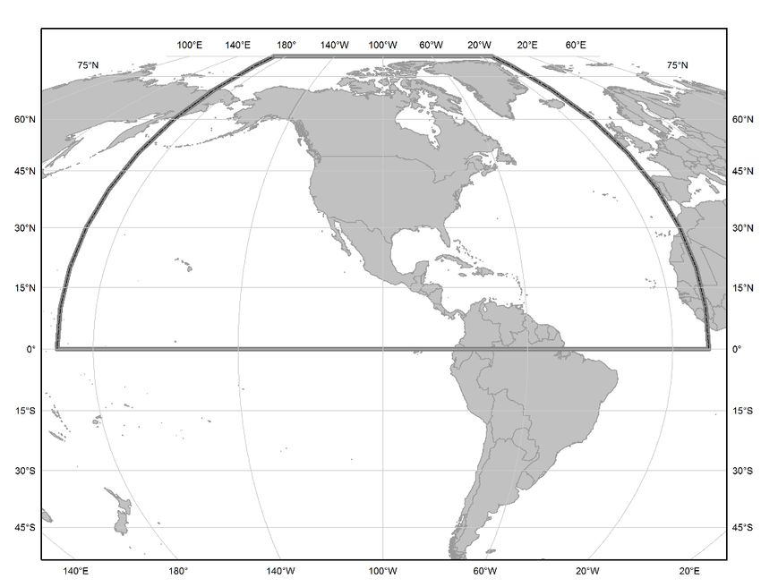
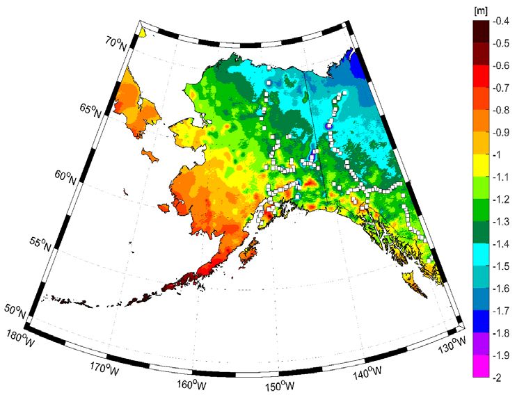
Figure 4-1: The continental bias and tilt of the NAVD 88 H=0 surface across CONUS as implied by the
latest NGS experimental geoid model based on improved gravity data.

Figure 4-2: The statewide bias and tilt of the NAVD 88 H=0 surface across Alaska as implied by the
latest NGS experimental geoid model based on improved gravity data. Note the tilt is due to the
severely poor distribution and quality of GNSS on Bench Mark data (white squares)

 9

A similar situation exists in Figure 4-2, however the southwest-northeast tilt in that grid covering Alaska
cannot be attributed to a tilt in NAVD 88 itself. This is because the network of NAVD 88 passive control
was never extended into western Alaska, and only marginally into eastern Alaska. Consequently, the
thin concentration of actual points with an NAVD 88 and a GNSS measurement resulted in wild
extrapolations of the conversion surface between the gravimetric geoid (USGG2012) and the hybrid
geoid (GEOID12B) in those regions. These extrapolations can only be called “the NAVD 88 H=0 surface”
per se, as they are a purely statistical anomaly and do not represent any actual leveling-based NAVD 88
data apart from the actual passive control shown in Figure 4-2. To summarize: the directionality and
degree of the tilt in Alaska is a byproduct of over-extrapolation in a data-sparse region 3 and should not
be considered a reflection of any “leveling-based NAVD 88 tilt” in Alaska.

Knowledge of the bias and tilt problem in NAVD 88, as well as uncertainty about the viability and
stability of the passive control network, led NGS to study the problem in preparation of the 2008-2018
NGS Ten-Year Plan (NGS, 2008). Estimates of the resources required to re-level the entire network were
extrapolated from existing labor and contracting costs. The estimate to completely re-level NAVD 88
ranged between $200 Million and $2 Billion dollars. It was concluded that—even if NGS could secure
funding at that level—re-leveling would not solve the underlying problems that (a) leveling builds up
large systematic errors over a continent, (b) passive control can move, unchecked, and (c) passive
control can easily be destroyed.

An entirely new approach was seen to be the only remaining viable option. Since the approximation in
equation 1 does not exceed 1 millimeter, and since GNSS-derived ellipsoid heights were accurate to
within a few centimeters anywhere in the United States, the only logical answer was for NGS to pursue
the creation of a geoid model more accurate than ever before realized (differentially 1-2 centimeters,
ideally). Furthermore, due to ground motion and stability uncertainty, the reliance upon passive control
as having “known heights” had to be replaced, with the determination of GNSS-derived ellipsoid heights
as the initial step in determining orthometric heights. This is the crux of NGS’s statements that CORS
would be the “primary access” and passive control the “secondary access” to the NSRS in the future.

5 Geoid Modeling - History

For over 4,000 years, humans have been referring to “heights” above the surface of some body of water.
One of the earliest extant records of this comes from about 2300 B.C.E. when, according to the Palermo
Stone (Hsu, 2010), the Egyptians regularly noted the “height” of the Nile River’s annual inundation.
While the exact datum those heights referred to is unclear, what is clear is that humankind has a long
history of thinking about heights relative to a body of water. But it was not until the 1800s that a
mathematical foundation for describing global mean sea level was developed. C.F. Gauss proposed a
“mathematical figure of the Earth” (Gauss, 1828), and G.G. Stokes built upon that idea to compute the

3
 Local errors (rather than the long wavelength tilt) are primarily caused by the difference between USGG2012
and xGEOID16B and are the result of actual data differences (updated satellite models and xGEOID16B included
GRAV-D airborne data, whereas USGG2012 did not).

 10

“surface of the Earth’s original fluidity” (Stokes, 1849). A few decades later, this mathematical
representation of sea level was given the name “geoid” (Listing, 1873).

For the better part of a century, modeling the geoid was pursued by mathematicians and geodesists,
though the practical application of that pursuit (using the modeled geoid as a reference surface for
heights) was limited by both data and theory. As late as 1967, one of the best known treatises
concerning the theory of geoid modeling claimed that “…an error of probably less than 1 meter in
[geoid undulation]…can be neglected for most practical purposes…” (Heiskanen and Moritz, 1967, p. 94).
Great strides have been made in data collection, computational power, and geoid modeling theory in
the intervening decades, to the point that negligible errors are now closer to the 1 millimeter to
1 centimeter level.

Because the geoid is a surface of equal gravity potential (see also section 6), the use of spherical
harmonics became a favored tool for modeling the geoid. 4 Essentially, spherical harmonics allow
modelers to easily represent a planetary-sized signal of infinite complexity with a simple series of
numbers; each number represents the power of the signal at a given spatial scale. The more numbers
used, the more detail is captured by the model. Readers interested in more detail are directed to Part 4
of this blueprint document and to Chapter 1 of Heiskanen and Moritz (ibid) or Hofmann-Wellenhof and
Moritz (2006). Through the 1970s and into the 1990s, a variety of ever-improving spherical harmonic
models (SHMs) were developed to describe the geoid. In the late 1990s, when the drive for centimeter-
accuracy in geoid models became a realistic goal, one of the weaknesses of SHMs became apparent—
the geoid exists within continental masses, in a place where potential fields are not harmonic (and thus
any “harmonic model” breaks down). SHMs were thus appended to include “correction coefficients” to
account for this non-harmonicity. One of these first examples was the Earth Gravity Model 1996
(EGM96; Lemoine, et al, 1998).

While SHMs continued to improve global models of the geoid, many countries were pursuing ever more
accurate geoid models for their particular region. In the United States, NGS developed GEOID90 (Milbert,
1991) and GEOID93 (NGS, 1993). The accuracy of these U.S.-specific geoid models could be checked by
using a significant amount of GNSS-derived ellipsoid heights in the NAD 83 reference frame and leveling-
derived orthometric heights in the NAVD 88 datum (see equation 1). It soon became apparent that the
geoid model based on gravity data and theory disagreed with the NAD 83 and NAVD 88 data at the level
of a few meters. The reasons for this were soon obvious: (1) the NAD 83 reference frame had a non-
geocentricity of over 2 meters, (2) the leveling-based heights were showing regional biases and tilts, and
(3) an overall bias was introduced by fixing the zero point of all of NAVD 88 to Local Mean Sea Level at just
one point on the St. Lawrence River (tidal station Father Point, Rimouski, Quebec, Canada). The conclusion
drawn by NGS was clear: if surveyors are using GNSS to obtain ellipsoid heights, and they want to use a
geoid model to transform those into orthometric heights, and if the surveyor is working in NAD 83 and
NAVD 88, then a purely gravimetric geoid model will not suffice.

In 1996, NGS began developing a two-track geoid modeling program. The best gravimetric geoid model
would be developed, but would then be modified to fit data from GNSS, and leveling in NAD 83 and

4
 The equation describing a 3-D gravity potential field is a differential equation. Spherical Harmonics are but one
kind of tool which can be chosen to solve this kind of differential equation. Other tools exist, such as ellipsoidal
harmonics. Further details are beyond the context of this document. Interested readers are directed to Chapter 1
of Heiskanen and Moritz (1967) or Hofmann-Wellenhof and Moritz (2006).

 11

NAVD 88. This modified geoid would be called a “hybrid geoid.” The first instance of this was the paired
G96SSS and GEOID96 models (Smith and Milbert, 1999). The pursuit of hybrid geoids has continued for
20 years, as NAD 83 and NAVD 88 remain the official datums of the NSRS. Hybrid geoids have served
many NSRS users well, yielding accurate NAVD 88 heights from GNSS (Roman and Smith, 2001; Roman,
et al, 2004; Wang, et al, 2011).

In 2007 NGS recognized both the growing trend of improved GNSS accuracy and the availability of that
accuracy to a broader range of users, as well as a significant new tool in the increased accuracy of geoid
modeling: airborne gravity. Furthermore, the national consistency and availability of a gravimetric
geoid model far surpasses the capabilities of passive control connected by leveling. Due to these
factors, the NGS Ten-Year Plan 2008-2018 (NGS, 2008) first laid out plans to replace NAVD 88 with a
vertical datum based on a gravimetric geoid model. The plan was described in the next NGS Ten-Year
Plan for 2013-2023 (NGS, 2013). Since that time, NGS has fleshed out how the entire geopotential
datum (including, but not limited to, using a gravimetric geoid as a zero-height surface) will be created
and will function, and the remainder of this blueprint document is dedicated to presenting those details.

6 The Geopotential Field

Some additional words should be said about a Spherical Harmonic Model (SHM) of Earth’s external
gravitational potential field in deference to the critical importance it has on the geoid model and many
other NGS products and services. However, a lengthy foray into this subject is inappropriate for the
scope of this document. Readers interested in greater detail or derivations are directed to the opening
chapters of Heiskanen and Moritz (1967) and Hofmann-Wellenhof and Moritz (2006) or any standard
textbook on Physics. Details in the remainder of this chapter are therefore limited to those essential to
the basic understanding of Earth’s geopotential field 5.

Let us begin with a few definitions:

 Gravitation: The force of attraction between two masses

 Centrifugal force: A ficticious force caused by the uniform circular motion of a body about some
 fixed point

 Gravity: The force acting on a body on or near Earth’s surface, which is a combination of the
 gravitational force and centrifugal fictitious force of Earth’s rotation

As evidenced by the above definitions, geodesists draw a clear distinction between gravitation and
gravity. This distinction will be important to note in this section.

Additionally, one must be cautious to draw distinction between the terms force, acceleration, potential
energy, and potential.

5
 Further details can be found in an NGS educational video “Gravity for Geodesy I: Fundamentals” available online
at https://www.ngs.noaa.gov/web/science_edu/online_lessons/

 12

6.1 Gravitation

The first force (of two which make up that which is called “gravity”) is gravitation. According to
Newton’s Law of Universal Gravitation, two point masses attract one another with a gravitational force
(F), directly proportional to the product of the two point masses (m1, m2) and inversely proportional to
the distance between them (s), squared, and directed along the straight line between the two masses.
Gravitational force therefore is a three-dimensional vector.

Geodesists have found it easier and more convenient to work with a related value, called gravitational
potential, (also called the gravitational potential energy per unit mass.) Gravitational potential is a
scalar value, directly proportional to some attracting mass, and inversely proportional to the distance to
that attracting mass:
 
 = (2)
 
The convenience of this quantity is that, being a scalar, it represents a single value (rather than vectors,
which would require magnitude and direction) in a field surrounding a mass. That statement is equally
true for a point mass or a set of point masses (such as a body, planet Earth, for example). That is, if one
added up equation 2 for every point mass that made up the Earth (using all the various distances to
those point masses), one can say that the Earth’s masses generate a gravitational potential field.
 
 ( , , ) = ∑ (3)
 ,( , , )

Equation 3 is the simplest form of the gravitational potential field of a body (such as the Earth), but is
effectively impractical to use as is.

Related to gravitational potential is gravitational acceleration. Similar to gravitational force,
gravitational acceleration is a three-dimensional vector, directed along the line between two point
masses. It is directly related to gravitational potential through the derivative with respect to the
separating distance s:
 
 ∗ ( , , ) = ∑ 2 (4)
 � ,( , , ) �

To summarize this section: Gravitational force (F) induces gravitational acceleration (g*), which is also
the gradient of gravitational potential (V).

 6.2 The Spinning Earth

In addition to experiencing the gravitational pull of the Earth, a body at rest on the Earth is also
experiencing a centrifugal fictitious force, 6 because it is moving in uniform circular motion as the Earth

6
 This quantity is traditionally called the “centrifugal force,” although it is not a “force” in the ordinary sense of the
word. “Fictitious forces or inertial forces arise from the inertial properties of matter rather than from the presence

 13

rotates. This fictitious force acts to thrust the body away from the point about which the circular
motion is happening (such as Earth’s axis of rotation.) Such a ficticious force would not exist if, for
example, the body were able to independently maintain its position in space while the Earth
spun nearby.

Like gravitational potential, it is convenient for geodesists to refer to centrifugal potential:
 1
 Φ( , , ) = 2 2 (5)
 2

Where ω is the angular velocity of the Earth and p the distance along a line normal to Earth’s spin axis to
the point. The acceleration due the centrifugal force is:

 a ( , , ) = 2 (6)

 6.3 Gravity

The combination of gravitational acceleration and centrifugal acceleration is called gravity acceleration:

 g = g ∗ + a (7)

Just as gravity acceleration (g) is the combination of gravitational acceleration (g*) and centrifugal
acceleration (ac), so too is gravity potential (W) the combination of gravitational potential (V(1)) and
centrifugal potential (Φ):

 = (1) + Φ (8)

For the remainder of this report the stand-alone use of “gravitation” will refer to gravitational
acceleration, and the stand-alone use of “gravity” will refer to gravity acceleration.

Spherical harmonic models (SHMs) of Earth’s external (specifically “above the masses”) gravitational
potential, such as EGM96 and EGM2008 (Pavlis, et al, 2008) are three-dimensional models of the scalar
potential, V, as seen in equation 3. These models are valid everywhere the potential is harmonic, true
everywhere where no solid mass exists (a.k.a. “outside the crust” or “external”). 7 SHMs are a common
(probably the most common) representation of the global gravitational potential field and fulfill this
equation (Smith, 1998) 8:
 
 ( )1 1 
 (1) ( ,
 , ) = ̅ ( ) + , 
 � � � � � , ̅ ( )� � , ( ) (9)
 
 =0 =0

of other bodies.” (Fowles, 1970). To put it another way, “Newton’s equation, F=ma, is only valid in an inertial
frame. A rotating reference frame is not inertial. If we transform Newton’s equation into a rotating frame,
additional non-inertial terms arise. These terms are not induced by any form of physical attraction, nor any
physical body. They arise due to the non-inertial motion of an observer.” (Marion, 1970).
7
 Astute readers will note that the atmosphere is not massless, nor are all of the astronomic bodies outside the
Earth. These issues are known and carefully accounted for, but details are not appropriate for this document.
8
 The superscript (1), in V(1), distinguishes the true gravitational potential from a simpler version called the “normal
gravitational potential,” designated V(2). See also Smith (1998) for details.

 14

̅
An SHM is a collection of fully normalized coefficient ( , ̅ ) and Legendre function ( � , )
 and , 
values for every degree and order (n and m), up to some maximum degree n=N value chosen by the
model-maker, as well as the GM1 and a1 values. 9 (See also Heiskanen and Moritz, 1967, Figure 1-9, or
Hofmann-Wellenhof and Moritz, 2006, Figure 1.5). Equation 9 can be used to calculate the gravitational
potential (up to that maximum degree N) at any point in spherical three-dimensional space (geocentric
radius r, spherical colatitude θ, longitude λ).

When geodesists speak of “equipotential surfaces” such as the geoid, they refer to surfaces of equal
gravity potential. That is, on the geoid, gravity potential (equation 8) is a constant, but not gravity
(equation 7).

What is elegant about an SHM (used in combination with equation 5, the centrifugal potential equation)
is that it can be used to calculate anything that is a function of gravity potential. In other words, once
you have an SHM of the gravitational potential, then you can also calculate the acceleration of gravity
(in all three directions), deflections of the vertical, and other related quantities. However, equation 9 is
an imperfect representation of Earth’s gravitational potential and is limited by three factors: first, it only
yields correct results at points that are in harmonic space (outside of the solid masses); second, it is
necessarily limited in spectral content (and therefore spatial resolution) by that maximum “n=N” value;
 ̅
and third, the , ̅
 and , values themselves are not perfectly determined and have error. That
second limitation is called “omission error,” while the third limitation is “commission error.”

The first limitation is dealt with, in part, by using digital elevation models (DEMs) to compute the
gravitational potential of topographic masses outside the geoid. This potential is “removed” to make
the field harmonic outside the geoid, and then “restored” after performing SHM computations.

One way to address the second limitation is to increase the N value, so that more detail is included in
the model, and it produces a better (in theory) representation of Earth’s gravitational potential. In
practice, “high-degree expansions,” with N = 20,000 or more, push the limits of current computing
power and challenge the integrity of equation 9. SHMs in use at NGS routinely use N values closer to
2,000 to balance the practical time needed to do the computations, versus the resulting model spatial
resolution. Switching from spherical to ellipsoidal harmonics has been shown to be a more stable
approach when dealing with such large-degree harmonic models.

The third limitation (“commission error”) is mitigated by using a complete spectrum of accurate sample
gravity data for determining the coefficients. That includes using satellite data for the long wavelength
field (≥ 250 kilometers), terrestrial gravity (and DEM computations) for short wavelengths (< 100
kilometers), and aerial gravity measurements for the medium wavelength field (20 to 300 kilometers).
Indeed, one of the main reasons for the Gravity for the Redefinition of the American Vertical Datum

9
 The values of GM and a do, ostensibly, have physical meaning. But ultimately, they function as scale factors in
equation 9 and therefore need not be perfect for equation 9 to be useful. Nevertheless, for completeness, the
value of GM has historically been the product of Newton’s gravitational constant times the mass of the Earth,
while a should be the radius of a sphere (such as Earth’s radius at the equator), outside of which there are no
masses. It should be pointed out that equation 9 tends to yield valid results for points inside a sphere of radius a,
provided there are no masses at, or above, the points being evaluated.

 15

(GRAV-D) project is to provide accurate measurements of the medium wavelength field (NGS, 2007).
GRAV-D is thus an essential part of creating the new geopotential datum.

Despite these limitations, an SHM is an incredibly powerful and fast tool for yielding a variety of gravity-
potential-related quantities anywhere on or outside the Earth’s crust. In the overwhelming majority of
regional geoid modeling efforts, such as GEOID93, etc., an SHM serves as the foundation of the model.
However, because the geoid itself resides in non-harmonic space, an SHM can never, by itself, yield a
model of the geoid, even if it were possible to set N=infinity.

Because an SHM describes potential at any point (r, θ, λ), it can be used to locate a surface of constant
potential. That is, given an SHM and equation 5, one can solve for the coordinates (r, θ, λ) of all points
fulfilling this condition for any given constant:

 = (10)

Surfaces fulfilling equation 10, having equal gravity potential, are referred to as equipotential surfaces.
The geoid, by definition, is that one equipotential surface which best fits global mean sea level. 10 When
a model of the geoid is created, one often begins with an SHM, which means a choice must be made
concerning which (of the infinitely many) equipotential surfaces is actually being modeled as “the geoid”
(Smith, 1998). Once such a choice is made, the numeric value of the constant must be chosen. That
value is often given the name W0, so that the geoid fulfills this condition:

 = 0 (11)

The role of SHM in 2022 will therefore be critical, as well as the role of W0, and both will be discussed in
section 9.

7 Time Dependency

Passive control is set into the crust of the Earth, which can move vertically, sometimes at relatively large
speeds (multiple centimeters per year). As such, the crust (and things set into it) makes a poor choice
for geodetic control, unless it is regularly monitored for movement. And while CORS is monitored
regularly for motion, its vertical movement is purely geometric (ellipsoid heights) and—due to the
changing nature of the geoid—cannot be directly equated to orthometric height changes (since
orthometric height changes are a combination of ellipsoidal height change AND geoid height change).

Although the geoid also changes vertically, its changes (relative to the magnitude of vertical crustal
changes) are smaller than ellipsoidal height changes. Geoid change requires large movements of mass,
such as the flow of extra material into the mantle below Hudson Bay, or the secular deglaciation of
Alaska, for the geoid change to be measurable on a yearly timescale (i.e. over 1 millimeter per year). In
addition, secular (relatively constant over time) change, episodic events (certain volcanic eruptions or
earthquakes), and some cyclic events (present-day ice melting of glaciers in Alaska and Greenland) can
affect the geoid in a measurable way. The long-term impact of these events can be either permanent or

10
 The fact that global mean sea level is changing will be addressed later.

 16

transient. An example of an episodic change with a permanent impact might be an earthquake, while
 an example of an episodic change with a transient impact might be a multi-year drought.

 NGS has begun investigating all potential physical processes which could modify the geoid over time.
 Each type of change will be investigated for three components: magnitude, temporal duration, and
 spatial scale.

 An example of some of the physical processes investigated is shown in Table 7-1. Those entries in red
 have already been determined to be too small for NGS to track. This table is meant to be illustrative,
 not exhaustive:

Type of Frequency Temporal Example Magnitude Spatial scale
Change Duration
Shape Secular Permanent GIA at Hudson Bay 2 mm / year > 100 km
 Deglaciation of Alaska
Shape Secular Permanent Slowing of Earth’s Spin Rate 8x10-17 mm / y Pole to Equator
Shape Periodic Permanent Seasonal Freeze/Thaw Cycles Being studied > 100 km
Shape Episodic Permanent Certain Earthquakes Being studied < 100 km
Shape Episodic Transient Droughts/Deluges Being studied Up to 500 km?
Size Secular Permanent Accretion of Space Dust 4x10-7 mm / y Global
Size Secular Permanent Loss of Stratospheric Mass -10x10-7 mm / y Global
W0 Secular Permanent Global Mean Sea Level 1.7- 3.2 mm / y 12 Global
 Change 11

 Table 7-1: Some of the geophysical drivers of geoid change.
 Entries in red will not be incorporated into NAPGD2022.

 Another factor to consider while studying sources of geoid change is that the sources can be grouped by
 the types of change they introduce to the geoid. These three types of geoid change are:

 1) Shape change: This means a change to the shape of the W=W0 surface, without changing W0
 itself and while maintaining the average radial distance from Earth’s center to the W=W0
 surface. If one considers W=W0 like a balloon, this is analogous to squeezing the balloon. Some
 new bulges and some new depressions will occur, affecting only the shape of the balloon, not
 its size.
 2) Size change: This means a change to the size of the W=W0 surface, effectively increasing (or
 decreasing) the volume enclosed by the geopotential field itself, without changing the value of
 W0. Continuing the balloon analogy from above, this would be akin to inflating or deflating the
 balloon without squeezing it.
 3) W0 change: This means that the surface which was called “the geoid” and had W=W0 will no
 longer be the geoid. A new value of W0 (W0new) is chosen, and “the geoid” is now the surface
 W= W0.new Continuing the balloon analogy, consider two balloons, a red one inside a green one,
 where both are inflated, but are not touching one another. A new W0 means the geoid was the

 11
 This particular signal only affects the value of W0 for the geoid if the geoid definition remains tied to GMSL.
 12
 While 1.7 millimeter per year was the average over the 20th century, the value has been accelerating and is now
 closer to 3.2 millimeters per year. See IPCC (2013).

 17

red balloon, but now you have chosen to make it the green balloon, without necessarily
 changing the size or shape of either.

NGS has set the ambitious target of maintaining geoid accuracy at 1 centimeter (1 standard deviation) in
both absolute and differential geoid undulations, but is also interested in balancing practicality against
that goal. That means that each of the signals above has been considered both for its spatio-temporal
scales, as well as its impact on users to determine which signals will be included in the dynamic portion
of the geoid model, DGEOID2022.

8 Sea Level Change

The standing definition of the geoid, as adopted and used at NGS is this:

 The geoid is the equipotential surface of the Earth's gravity field which best fits, in a least
 squares sense, global mean sea level.

This definition, like many geodetic specifications, was highly suitable and stable for decades. And like
many geodetic specifications, the accuracy to which geodesists measure things has made it necessary to
re-think this definition. To be specific, over a century of sea level measurements have made it ”very
likely” that global mean sea level (GMSL) is rising at a rate of approximately 3.2 millimeters per year
(IPCC, 2014).

NGS has set an accuracy goal for geoid models in the future of 1 centimeter (at 1 standard deviation or
“sigma,” about 68 percent confidence) in both absolute and relative (over all distances) geoid height. If
NGS were to continue to stand by the geoid definition above, then as GMSL rises, so must its best fitting
geopotential surface. That is to say, as GMSL rises, so must the geoid; and thus all orthometric heights
must get smaller, year by year. To be clear, as GMSL rises, the value of gravity potential which best fits
to GMSL (called W0) will also change.

To be sure, any change of sea level also has a component of mass re-distribution, which means there is
also a component of shape change, not just W0 change, as part of this. To exemplify the subtlety of the
two types of change that will come from the one issue (sea level change), consider the following
example.

Figure 8-1 and Figure 8-2 illustrate schematically what happens over time with GMSL and the potential
field. Specifically, the rise of GMSL is not purely geometric. Masses have re-distributed on the Earth
(due to addition of water mass to the oceans, loss of water mass from land ice, and thermal expansion
of the ocean waters themselves). Thus the shapes of equipotential surfaces in the old potential field,
W(t0), will not necessarily be the shapes of equipotential surfaces in the new potential field, W(t1).
Furthermore, when selecting the equipotential surface which best fits the new GMSL, there is no
guarantee that the previous numerical value of potential, W0, will be the same as the new numerical
value. In fact, it can be proven that the value will change, but that derivation is too lengthy for
this report.

There are arguments against maintaining the above definition of “the geoid.” The first is simply the
disruptiveness of an ever-changing geoid and thus ever-changing orthometric heights. However, since

 18

NGS is committed to providing scientific accuracy in its products and services, it seems to be a poor
choice to ignore the reality of sea level change.

At first glance, it would seem an argument is being made between two different geoid definition
scenarios: one where the geoid is definitionally tied to GMSL, and one where it is not. These two
scenarios are outlined in figures 8-3 and 8-4.

 Figure 8-1: Within the potential field which exists at time t0, W(t0), one particular
 equipotential surface in that field fits to the Global Mean Sea Level at time t0, GMSL(t0),
 has a constant value of potential “W0,” and is called “the geoid.”

 Figure 8-2: At time T=t1, GMSL rise comes with a mass re-distribution, so that the potential field
now, W(t1), differs from W(t0) in its equipotential shapes. Furthermore, the equipotential field which
 fits to GMSL will no longer have value W0. The dashed lines represent the lines seen in figure 8-1.

 19

Figure 8-3: Scenario 1 – the geoid definition remains tied to GMSL

Figure 8-4: Scenario 2 – the geoid definition disconnected from GMSL

 20

Both methods have advantages and disadvantages.

While there is no international standard, per se—the International Association of Geodesy (IAG) has
never defined the geoid—a reasonable way forward has been proposed by Laura Sanchez, chair of the
Joint Working Group on Strategy for the Realization of the International Height Reference System (IHRS)
of the IAG, in a recent paper (Sanchez, et al, 2016):

 “…a suitable recommendation is to adopt a potential value obtained for a certain epoch as the
 reference value W0 and to monitor the changes of the mean potential value at the sea surface
 WS. When large differences appear between W0 and WS (e.g., > ± 2 m2 s−2), the adopted W0 may
 be replaced by an updated (best estimate) value.”

This strategy will be adopted at NGS. What this means is that NGS will adopt Scenario 2, above, until the
geoid and GMSL have diverged by some threshold amount. When that threshold is reached a new geoid
will be defined and held fixed for a number of years. In this way, the impact of the change of GMSL is
accounted for in the heights of the NSRS, while the appearance of stability is maintained for decades at
a time (See Section 14). A simplistic view of this approach is presented in Figure 8-5.

 Figure 8-5: Scenario 3 - A new geoid is introduced
 whenever GMSL rises above some TBD threshold level

 21

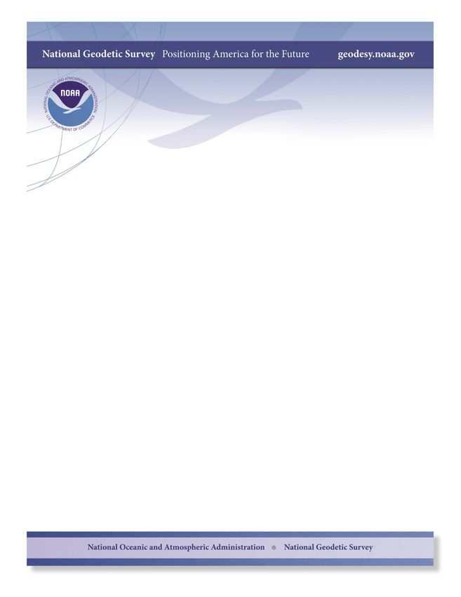
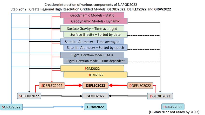
9 The 2022 Geopotential Datum

The National Geodetic Survey, in preparing for the 2022 replacement of NAVD 88 and all other vertical
datums in the NSRS, received user feedback through multiple channels (particularly through three
Geospatial Summits, in 2010, 2015, and 2017). In 2016 and 2017, reflecting on user feedback and
considering the right mix of science and stewardship, NGS held a number of internal and external
debates and discussions in an attempt to rigorously define the new geopotential datum for 2022.
The result of those discussions can be summed up as follows.

Note that many names in this document have not yet been finalized, however working names are
provided for clarity of discussion.

 1) In 2022, the NSRS will contain one geopotential datum, capable of providing (at a minimum) the
 geoid undulation, acceleration of gravity, geopotential number, and deflection of the vertical at
 any given latitude, longitude, ellipsoid height, and time in a global ideal reference frame, such as
 the International Terrestrial Reference Frame (ITRF) or International GNSS Service (IGS) frames.
 The name of this datum will be the North American-Pacific Geopotential Datum of 2022
 (NAPGD2022).
 2) The foundational component of NAPGD2022 will be a spherical 13 harmonic model of Earth’s
 external gravitational potential, called (for now) the Geopotential Model of 2022 (GM2022).
 The GM2022 will be created for the entire Earth and will contain two components:
 a. The first component will be time independent, fixed at some epoch (TBD 14) to a at least
 degree and order of 2160, 15 called (for now) the Static Geopotential Model 2022
 (SGM2022).
 b. Complementing SGM2022 will be a time-dependent model of Earth’s external
 gravitational potential, capable of capturing both secular and episodic changes of
 significance. This time-dependent model will be called (for now) the Dynamic
 Geopotential Model 2022 (DGM2022).
 3) Three derivative products, based upon GM2022, but requiring additional information and
 providing higher-resolution regional information than is contained in GM2022 will be created:
 a. A gridded geoid model GEOID2022, 16 which will contain two components:
 i. The first will be time independent, fixed at some epoch (TBD) called (for now)
 the Static Geoid model of 2022 (SGEOID2022).

13
 There is also a chance the model will be developed in ellipsoidal, rather than spherical, harmonics. Although the
basic application is the same, the increased stability of ellipsoidal harmonics at ultra-high degrees makes it an
appealing option. This decision will be made and announced prior to 2022, pending the results of ongoing
research.
14
 Valid arguments can be made for a variety of different epochs. For the sake of simplicity and balance, one may
argue, for instance, that this should be the reference epoch of the four new terrestrial reference frames (NGS,
2017). While true, there is no significant scientific reason these two epochs must be the same.
15
 Many current state-of-the-art SHMs have a maximum degree of 2160.
16
 The final GEOID2022 model will be a joint effort between the National Geodetic Survey, the Canadian Geodetic
Survey, and Mexico’s Instituto Nacional de Estadística y Geografía. The final methodology remains to be
determined (TBD), but these three agencies have been working closely on this project for years and have mutually
agreed to produce one single model in 2022.

 22

ii. Complementing this will be a time-dependent geoid undulation model,
 encompassing permanent geoid changes >= 1 millimeter per year, called the
 Dynamic Geoid model of 2022 (DGEOID2022).
 b. A gridded deflection of the vertical, DoV, model (at the surface of the Earth)
 DEFLEC2022, which will contain two components:
 i. The first will be time independent, fixed at some epoch (TBD) called (for now)
 the Static Deflection of the Vertical model of 2022 (SDEFLEC2022).
 ii. Complementing this will be a time-dependent DoV model, called the Dynamic
 Deflection of the Vertical model of 2022 (DDEFLEC2022).
 c. A model for interpolating surface gravity GRAV2022, which will contain at least one,
 possibly two components:
 i. The first will be time independent, fixed at some epoch (TBD) called (for now)
 the Static Gravity model of 2022 (SGRAV2022).
 ii. As a second, possible component, NGS will investigate the feasibility of a time-
 dependent surface gravity model.
 4) Software capable of using GM2022 to compute user-requested aspects of the geopotential field
 existing external to the crustal masses (including, but not necessarily limited to gravity,
 geopotential/spheropotential separations, surface deflections of the vertical, and geopotential
 numbers) will be built into NGS products and services.
 5) The GM2022 model, being global, can be evaluated to provide estimates of any geopential-
 related quantity, within any NGS product or service in the world (such as positioning with the
 Online Positioning User Service, OPUS), without regard to its location. Certain geopotential-
 related quantities, specifically geoid undulations, surface deflections of the vertical and surface
 gravity will, however, be evaluated with higher accuracy than is possible in GM2022, when
 within distinct regions (see #6 below).
 6) The three derivative, gridded products (GEOID2022, DEFLEC2022, and GRAV2022) will
 encompass three non-global areas. These three areas will be (latitude and longitude convention
 being positive north, positive east):

 Area North (°N) South (°N) West (°E) 17 East (°E)
 North America 90 0 170 350
 Guam and CNMI 22 11 143 148
 American Samoa -10 -16 186 193

 For the North American region specifically, boundaries were determined by first assuring that
 certain areas (CONUS, Alaska, Hawaii, Canada, Mexico, Central America, the Caribbean, and
 Greenland) were contained in the computational area. Then an appropriate buffer was added
 to avoid “edge problems” during the computation.

 Only within these three regions will an OPUS solution (or other NGS product or service) yield a
 geoid undulation, deflection of the vertical and surface gravity value in NAPGD2022.

17
 The longitude system chosen here is a 0-360, positive east system. This avoids a few problems, including (a)
mixing positive and negative longitude values, (b) using a west longitude system with values larger than 180, which
seems to be a United States-specific invention, and (c) the need to specify an alphabetic hemisphere.

 23

Figure 9-1: The North American region for GEOID2022, DEFLEC2022 and GRAV2022

Figure 9-2: The American Samoa region for GEOID2022, DEFLEC2022 and GRAV2022

 24

Figure 9-3: The Guam and CNMI region for GEOID2022, DEFLEC2022, and GRAV2022

9.1 Relationship between GEOID2022 and Other Height Reference Surfaces

GEOID2022 will be the official zero-height surface for orthometric heights within NAPGD2022, and thus
within the NSRS. However, other types of heights and other types of reference surfaces are used
throughout the world, and their relationship to GEOID2022 should be accurately understood.

 25

Global Mean Sea Level (GMSL): This was already touched upon, but some further clarification is due.
Specifically, the SGEOID2022 portion of GEOID2022 should be considered to best fit global mean sea
level at the (TBD) reference epoch of NAPGD2022, within the bounds of known errors and acceptable
error tolerances. The DGEOID2022 portion of GEOID2022 will track changes to the shape of the geoid,
but will not contain any element of the approximately 3 millimeters per year GMSL rise (IPCC, 2014; for
more details, see sections 8 and 14).

Local Mean Sea Level (LMSL): Local Mean Sea Level can behave very differently from GMSL.
Additionally, LMSL behavior can vary significantly between neighboring coastal locations. Consequently,
any LMSL change (rise or fall) may be different than the GMSL change rates. Heights above LMSL at
various tidal datums (Mean High Water, Mean Lower Low Water, etc.) are of critical importance for
navigation and flood risk determination. But heights on most topographic maps are generally
orthometric, unrelated to LMSL. It is therefore important for a relation to exist between NAPGD2022
heights and LMSL heights. Such ties will best be determined by using GNSS technology at tide gauges.
Between tide gauges, NGS will work with NOAA’s Center for Operational Oceanographic Products and
Services (CO-OPS) to provide interpolation tools (akin to the current VDatum tool). The LMSL heights
are usually tied to a group of local tidal benchmarks through a short leveling survey. Using GNSS
surveying at the same points, NAPGD2022 orthometric heights can be determined.

North American Datum of 1988 (NAVD 88), et al: Until replaced in 2022, 18 NAVD 88 is the official
vertical datum of the NSRS in CONUS and Alaska. Other official vertical datums exist in Puerto Rico
(PRVD02), the U.S. Virgin Islands (VIVD09), American Samoa (ASVD02), The Commonwealth of the
Northern Mariana Islands (NMVD03), and Guam (GUVD04). A transformation tool (an update of the
existing VERTCON tool) will be built which transforms orthometric heights in each of these datums into
heights in NAPGD2022. A campaign is underway at NGS to collect GNSS data on benchmarks in each of
these datums to assist in building the new version of VERTCON. 19

International Great Lakes Datum (IGLD): The IGLD is an international vertical datum jointly defined and
realized by the United States and Canada. The IGLD uses dynamic heights, which are relative
geopotential values converted to units of length (equivalent to “hydraulic head” used in engineering).
The reason for this type of height is that a change in dynamic height equals a change in hydraulic head,
which more accurately indicates water levels and flow than orthometric height differences—an
important characteristic for the Great Lakes. The current realization, IGLD 85, was co-defined with
NAVD 88 (they both are derived from the same set of geopotential numbers, adjusted from geodetic
leveling and surface gravity measurements), although NAVD 88 dynamic heights are generally not
numerically equal to those of IGLD 85. The reason for the difference is that IGLD 85 dynamic heights are
“corrected,” so that they match lake levels at official water level stations at an epoch of 1985 (the mid-
year of a standard seven-year observation period). A new realization, IGLD2020, will be centered on
water level epoch 2020, so it will not be available until after the end of the water level observation

18
 Although the National Geodetic Survey will define NAPGD2022, it will not become the official replacement for
NAVD 88 until it is approved by the Federal Geodetic Control Subcommittee.
19
 Hawaii has never had an official vertical datum defined as part of the NSRS. However, there is an effort
underway (circa 2017) to define a leveling-based datum in the state, on an island-by-island basis. Should any
component of that datum become an official part of the NSRS (either before or after 2022), then VERTCON will
also have a transformation tool from that Hawaiin vertical datum to NAPGD2022.

 26