Predicting Drought and Subsidence Risks in France - arXiv
←
→
Page content transcription
If your browser does not render page correctly, please read the page content below
Predicting Drought and Subsidence
                                                               Risks in France
                                                    Arthur Charpentiera∗ , Molly Jamesb & Hani Alic
arXiv:2107.07668v1 [stat.AP] 16 Jul 2021

                                           a
                                               Université du Québec à Montréal (UQAM), Montréal (Québec), Canada
                                                b
                                                    EURo Institut d’Actuariat (EURIA), Université de Brest, France
                                                                       c
                                                                           Willis Re, Paris, France
                                                        ∗
                                                            Corresponding author charpentier.arthur@uqam.ca

                                                                               July 2021

                                                                                 Abstract
                                               The economic consequences of drought episodes are increasingly im-
                                           portant, although they are often difficult to apprehend in part because
                                           of the complexity of the underlying mechanisms. In this article, we will
                                           study one of the consequences of drought, namely the risk of subsidence (or
                                           more specifically clay shrinkage induced subsidence), for which insurance
                                           has been mandatory in France for several decades. Using data obtained
                                           from several insurers, representing about a quarter of the household in-
                                           surance market, over the past twenty years, we propose some statistical
                                           models to predict the frequency but also the intensity of these droughts,
                                           for insurers, showing that climate change will have probably major eco-
                                           nomic consequences on this risk. But even if we use more advanced models
                                           than standard regression-type models (here random forests to capture non
                                           linearity and cross effects), it is still difficult to predict the economic cost
                                           of subsidence claims, even if all geophysical and climatic information is
                                           available.

                                           Keywords: clay shrinkage; drought; France; insurance; natural catastro-
                                           phes; prediction; subsidence; zero-inflated

                                           Acknowledgement: The authors wish to thank Hélène Gibello, Sonia
                                           Guelou, Florence Picard and Franck Vermet for comments on a previ-
                                           ous version of the work. Arthur Charpentier received financial support
                                           from the Natural Sciences and Engineering Research Council of Canada
                                           (NSERC-2019-07077) and the AXA Research Fund.

                                                                                     1
1     Introduction
For the insurance industry, climate change is a challenge since risks are increas-
ing, in terms of frequency and intensity, as discussed in McCullough [2004], Mills
[2007], Charpentier [2008] or Schwarze et al. [2011]. In this article, we will see
if it is possible to predict, for a given year, the costs associated with drought,
and more specifically here, clay shrinkage induced subsidence, in France.

1.1    Drought and climate change
In a seminal book published twenty years ago, Bradford [2000] started to ad-
dress the problem of getting a better understanding of the connections between
drought and climate change, already suggesting that the frequency and the in-
tensity of such events could increase in the future. And in the more recent
book, Iglesias et al. [2019] provided additional evidence about the influence
of climate change on meteorological droughts in Europe. Ionita and Nagav-
ciuc [2021] studied the temporal evolution of three drought indices over 120
years (the standardized precipitation index – SPI, the standardized precipita-
tion evapo-transpiration index – SPEI, and the self-calibrated Palmer drought
severity index – scPDSI). This updated study regarding the trends and changes
in drought frequency in Europe concluded that most of the severe drought events
occurred in the last two decades, corresponding to the time after the publica-
tion of Lloyd-Hughes and Saunders [2002], for example. Similarly, Spinoni et al.
[2015] and Spinoni et al. [2017] (studying more specifically Europe, following
their initial, all over the world in Spinoni et al. [2014]) observed that for both
for frequency and severity, the evolution towards drier conditions is more rele-
vant in the last three decades over Central Europe in spring, the Mediterranean
area in summer, and Eastern Europe in autumn (using also multiple indices,
over 60 years).
    Regarding economic impacts, Hagenlocher et al. [2019] provided a state of
the art of scientific publications over the past twenty years (presenting the out-
comes of a systematic literature review of people-centered drought vulnerability
and risk conceptualization and assessments). Naumann et al. [2021] shows that
(in Europe), drought damages could strongly increase with global warming and
cause a regional imbalance in future drought impacts. They provide some fore-
casts, under the assumption of absence of climate action (+4◦ C in 2100 and no
adaptation), annual drought losses in the European Union and United Kingdom
combined are projected to rise to more than 65 billion e per year compared with
9 billion e per year currently, still two times larger when expressed relative to
the size of the economy. Note that this corresponds to the general feeling of the
insurance industry: Bevere and Weigel [2021] suggests that, regarding climate
change, drought trends and socio-economic factors, not only will it persist, but
even accelerate further.
   But at the same time, Naumann et al. [2015] pointed out that related direct
and indirect impacts are often difficult to quantify. A key issue is that the

                                        2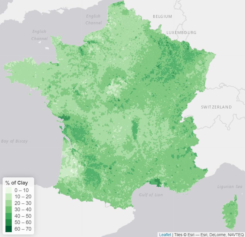
lack of sufficient quantitative impact data makes it complicated to construct a
robust relationship between the severity of drought events and related damages.
Insurance coverage for drought has been intensively studied, when related to
agriculture. Iglesias et al. [2019] mentions some drought insurance schemes, with
either indemnity based mechanisms, but also drought index based insurance, in
Section 2.8. Vroege et al. [2019] provides an overview of index-based insurances
in Europe and North America, in the context of droughts, while Bucheli et al.
[2021] focuses on Germany. Note that Tsegai and Kaushik [2019] addresses
the importance of designing insurance products which does not only address
drought impacts but also minimize land degradation. Besides this theoretical
work, some countries provide actual covers for such risks. For example in Spain,
it is possible to insure rain-fed crops against drought, as discussed in Entidad
Estatal de Seguros Agrarios (ENESA) [2012], but in most country, drought
coverage is only concerned with respect to agricultural (crop) insurance, as
such as frost (see also Pérez-Blanco et al. [2017]).

1.2    From drought to subsidence
In this article, we will use data from several insurance companies in France,
regarding a very specific drought related risk, that is clay shrinkage induced
subsidence (even if we predict only a part of the evaluation of cost assessment
of land subsidence, as pointed out in Kok and Costa [2021]). If clay shrinkage in-
duced subsidence is now a well known risk (or at least recognized as a major risk,
see for instance Doornkamp [1993], or Brignall et al. [2002] which assessed the
potential effects of climate change on clay shrinkage-induced land subsidence),
insurance coverage for subsidence is still uncommon. Almost twenty years ago,
as indicated in McCullough [2004], while perils related to earth movement were
traditionally excluded from most property policies, several states (in the United
States of America) have mandated coverage for some subsidence related claims
(with several limitations). And recently, Herrera-Garcı́a et al. [2021] proved that
subsidence permanently reduces aquifer-system storage capacity, causes earth
fissures, damages buildings and civil infrastructure, and increases flood suscep-
tibility and risk. From an insurer’s perspective, Wües et al. [2011] pointed out
that as incidents of soil subsidence increase in frequency and severity with cli-
mate change, there is a need for systematic managing of the risks through a
combination of loss prevention and risk transfer initiatives (such as insurance).
    In France, subsidence is a phenomenon covered by all private property insur-
ance covers, and that enters the scope of the government backed French natural
catastrophe regime provided by the Caisse Centrale de Réassurance (CCR). It
is the second most important peril in terms of costs that the system covers (the
first being floods, see Charpentier et al. [2021] for a recent discussion about
flood events in France, in the context of climate change). Subsidence risk is
defined (Ministère de la transition écologique et solidaire (MTES) [2016]) as
the displacement of the ground surface due to shrinkage and swelling of clayey
soils. It is due mainly to the presence of clay in the soil which swells in hu-

                                        3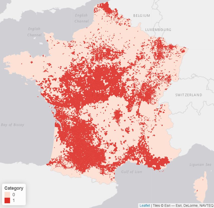
mid conditions and shrinks in dry ones, thus creating instabilities in the terrain
under constructions causing cracks to appear on the floor and walls which can
jeopardise the solidity of the building. France, having a temperate climate, has
saturated clayey soils, making subsidence predominant during droughts.
    However, the past few years have seen this risk exacerbated by the extreme
heat waves and lack of rainfall in France (see Caisse Centrale de Réassurance
(CCR) [2019]), causing more and more subsidence claims, with little hope of this
tendency stopping, given the current climate change context. Indeed, since 1989,
38% of the total costs of claims are concentrated over the period 2015-2019, that
is 15% of the total time that subsidence coverage has been in place (as discussed
in Mission des Risques Naturels (MRN) [2021]). Furthermore, Soubeyroux et al.
[2011] shows that the frequency and intensity of heat waves and droughts will
inevitably increase in the coming century in continental France and new areas
that so far have been protected from drought will be at risk. Additionally, AFFA
[2015] predicts that the cost of geotechnical droughts will nearly triple in 2040.
More recently, the French Geological Survey (BRGM, Bureau de Recherches
Géologiques et Minières) published a study, Gourdier and Plat [2018], describing
extreme historical subsidence events as well as forecasts using various climate
change scenarios. It found that the first third of the century will suffer from
unusual droughts in both their intensity and spatial expansion: one in three
summers between 2020 and 2050 and one in two summers between 2050 and
2080 are to be as extreme as the summer of 2003 in continental France (the worst
subsidence event ever registered by the CCR, see Corti et al. [2009] that focused
on the 2003 heatwave in France). Looking at the most pessimistic scenario, a
2003 type event might occur half of the time between 2020 and 2050. One
should recall that in 2003, the heat wave caused damage due to the shrinking
and swelling of clay, for which compensation (via the natural disaster insurance
scheme, and then via an exceptional compensation procedure for rejected cases)
was estimated at approximately 1.3 billion e in Frécon and Keller [2009], while
over the period 1989-2002, the average annual cost of geotechnical drought for
the natural disaster insurance scheme was more than five times smaller, with
205 million e.
    Furthermore, subsidence is a risk with a long declaration period, with on
average 80% of the number of claims declared two years after the event. This
delay is due to the lengthy acceptance process of subsidence natural catastrophe
declarations, upon which the validity of most claims is dependant. Although
most insurers are reinsured against this peril with the CCR, the retention rate
remains high (50%), it is thus necessary for insurers to develop their own view
of this risk in order to estimate their exposure to this growing hazard. However,
the inherent characteristics of subsidence make it a risk that is complex to
model: it has slow kinetics and an absence of precise temporal definition, making
subsidence models sparse on the market.
    Bevere and Weigel [2021] mentioned since 2016, annual inflation-adjusted in-
sured losses have continuously exceeded 600 million e, with an average annual
loss close to 850 million e, which corresponds to around 50% of the CatNat

                                        4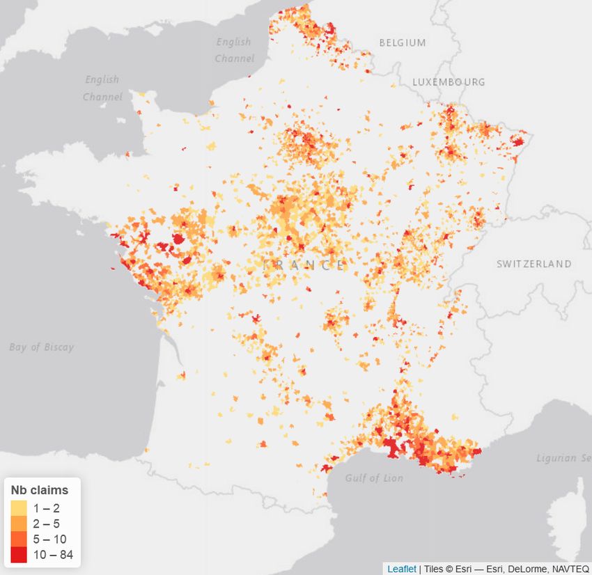
premiums collected, and makes subsidence possibly one of the most costly nat-
ural risk in France. Overall, a high to medium clay shrink-swell hazard affects
one-fifth of metropolitan France’s soils and 4 million individual houses, as men-
tioned in Antoni et al. [2017]. And Soyka [2021] mentioned that this is not just
in France, increased subsidence hazard gains attention in other countries, too
(even if this article focuses solely on France).

1.3        Agenda
The purpose of this study is to provide a regression-based model that will allow
to predict annual frequency and severity of subsidence claims to be made, based
on market data and climatic indicators. The model created in this study bases
future predictions on past occurrences, thus a historical insurance database was
necessary to calibrate the models, alongside indicators of the severity of his-
torical events that could be reproduced into the future. These indicators were
created using climatic and geological data that capture the specifics of past
events and regional information. The creation of this database and the choice
of indicators will be described in section 2. Using this historical data, various
models are implemented, chosen to adapt to the particularities of the data, in
order to improve the precision of the predictions. There will be three layers to
model the costs of subsidence claims (1) a drought event should be officially
recognised (corresponding to a binary model, specificities of the French insur-
ance scheme will be discussed in the next section) (2) if there is a drought, the
frequency is considered (corresponding to a counting model, classically a Poisson
model) (3) for each claim the severity is studied (corresponding to a cost model,
here some Gamma model). As we will see, using so-called zero-inflated mod-
els, the first two models can be considered simultaneously. Various tree based
models were also tested in an attempt to obtain more realistic predictions. In
section 3, we will present those models, and we will analyse predictions obtained
on the frequency, and more specifically discuss the geographical component of
the prediction errors. And finally, in section 4, we will present some models to
predict to total costs of subsidence events, in France, and again, study mode
carefully the prediction errors, in 2017 and 2018.

2         Subsidence risk in France and our dataset
A yearly claim and exposure dataset, sourced from several different French in-
surers, relative to Multi-Peril Housing Insurance (Multi-Risque Habitation) for
individual houses in metropolitan France, for the period 2001 to 2018, was
used here for frequency and severity of past events. This dataset was enriched
with additional information based on geophysical indices usually used to model
droughts.
        Our dataset was aggregated at the town level1 , with no information about the
    1   Here, we use here the word “town” to designate a “commune” (in French), or “munic-

                                              5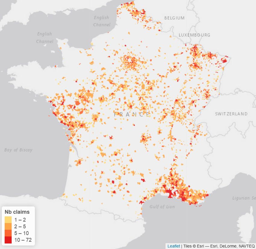
particularities of each individual contract that could influence the claims (such
as number of stories, size, orientation, etc.), creating the need for additional
information about the inherent risks of the town and its climatic and geophysics
exposure. One of the main issues when modelling subsidence is the absence of
precise temporal and geographical definition of a subsidence events. Thus, to
combat these issues, indicators must be created to grasp the geographical and
temporal characteristics of past events.
    In Section 2.1, after describing briefly the specificity of the French insur-
ance scheme, we will explain the variables of interest we will model afterwards,
namely the occurrence of a natural disaster (based on official data in France),
the number of houses and building claiming a loss, and the amount of the losses
(those last two based on data from three important insurance companies in
France, representing about 20% of the French market). Then, in Section 2.2
and 2.3, we will describe possible explanatory variables (for the occurrence of
a disaster, the percentage of houses claiming a loss and the severity). And fi-
nally, in Section 2.4 we discuss the use of other variables, mainly geophysical
information since we want to predict subsidence, and not droughts in general.

2.1    Specificity of the French Catnat system
The French “Régime d’Indemnisation des Catastrophes Naturelles” (also called
the “CatNat regime”) started in 1982 (see Charpentier et al. [2021] for an his-
torical perspective), even if drought damages were added to the (informal) list
of perils in 1989, as explained in Magnan [1995] or more recently Bidan and
Cohignac [2017]. The main idea of the mechanism is that any property damage
insurance contract, for individuals as well as for companies, includes manda-
tory coverage for natural disasters. The assets concerned are buildings used for
residential or professional purposes and their furniture, equipment, including
livestock and crops, and finally motor vehicles. These assets are insured by
multi-risk home insurance, multi-risk business insurance and motor vehicle in-
surance. The contractual guarantees (storm, hail and snow, fire...) are also very
often attached to household and business contracts. Livestock outside the barn
and unharvested crops, on the other hand, are covered differently. It should be
stressed here that the respective scope of insurable and non-insurable risks is
not defined by law, but is established by case law. Indeed, the natural disaster
insurance system is said to be “à péril non dénommé” (or unnamed peril) in the
sense that there is no exhaustive list of all risks that are covered. The effects
of natural disasters are legally defined in France as “uninsurable direct material
damage caused by the abnormal intensity of a natural agent, when the usual
measures to be taken to prevent such damage could not prevent their occurrence
or could not be taken” (article L.125-1 of the insurance legal code). In practice
(and it will be very important in our study) the state of natural disaster is
established by an interministerial order signed by the Ministries of the Interior
ipality”. There are 37,613 towns in metropolitan France (as characterized by their INSEE-
“commune” code).

                                           6
and of Economic Affairs. This order is based on the opinion of an intermin-
isterial commission. This commission analyzes the phenomenon on the basis
of scientific reports and thus establishes jurisprudence regarding the threshold
of insurability of natural risks. More specifically, in the context of our study
regarding drought, requests for recognition of the state of natural disaster are
examined for damage caused by differential land movements due to drought and
soil rehydration. And a list of towns that have been declared a natural disaster
are listed and associated guaranties are then applied, both for individual and
commercial policyholders, by (private) insurance companies.
In comparison to other natural catastrophes, subsidence has certain partic-
ularities. From an insurance point of view, the typical event-based definitions
of a natural catastrophe, that is possible for cyclones or avalanches, does not
apply. Indeed, it has slow kinetics, making it difficult to determine direct links
of causality between the event and the claims. Damage can be caused long after
the dry periods. However, that link of causality is the very definition of natural
catastrophe recognition which makes the implementation of different criteria to
determine the causality link of the event essential.
Subsidence was first observed, as a major risk, in France after the drought
of 1976 which caused important damage to buildings. After a similar event
in 1989, subsidence was integrated into the French natural catastrophe regime,
in the sense that policyholders can claim a loss to their insurance companies.
According to Mission des Risques Naturels (MRN) [2019], between 1989 and
2018, more than 11,300 towns have requested natural catastrophe recognition for
subsidence and over 9,500 were granted it. The natural catastrophe declarations
are published on average 18 months post-event, instead of 50 days for other
natural catastrophes and the duration of an event is on average of 50 days for
subsidence and of 5 days for other perils (like floods, avalanches or landslides,
among many others). The total cost of subsidence losses reached 11 Billion e
mid-2018, which is roughly 16,300e per claim. The number of towns that have
had their request declined has increased since 2003. Overall, the proportion
of acceptance is of 61%, however, just taking years subsequent to 2003, the
proportion is of only 50%. As mentioned earlier, this might be explained by the
fact that, according to the law, those events should be caused by “the abnormal
intensity of a natural agent ”. Thus, if a town is claiming losses every years, it
ceases to be “abnormal ”, and claims might be rejected then.
The evolution of the number of natural catastrophes since 1989, which is
the year of the oldest natural catastrophe in the dataset, shows that since the
1990s, the number of orders has been quite variable, however, 4 years seem to be
abnormally hardly-hit: 2003, 2005, 2011 and 2018. Note finally that Wües et al.
[2011] claims that, since subsidence and drought are related to temperature,
climate change will increase frequency and intensity of drought.
72.2 General considerations regarding drought indices
There exists many different options in terms of drought indicators to characterise
their severity, location, duration and timing (see Svoboda and Fuchs [2016] for
some exhaustive descriptions). The impact of droughts can vary, depending on
the specificities of each drought, captured differently by each indicator. It is
thus important to select an indicators with its application in mind. However,
the availability of data also plays an important role in the selection, as it limits
which indicator can be constructed.
The criteria to characterise the severity of shrinkage-swelling episodes evolved
in 2018, as the old criteria were outdated and overly technical, making them
difficult to interpret and explain to the public, see Ministère de l’intérieur (MI)
[2019]. The new system is based on two factors:
• A geotechnical factor pertaining to the presence of clay at risk of swell-
shrink phenomenon, in place since 1989. This criterion enables the identi-
fication of soils with a predisposition to the phenomenon of shrinkage-
swelling depending on the degree of humidity. The analysis is based
on technical data established by the Bureau des Recherche Géologiques
et Minières (BRMG), see Ministère de la transition écologique et sol-
idaire (MTES) [2016]. Areas of low, medium and high risk are considered
to determine whether the communal territory covered by sensitive soils
(medium and high-risk areas) is greater than 3%. This will be discussed
in Section 2.4. However, the intensity of shrinkage-swelling is not only due
to the characteristics of the soil but also to the weather.
• A meteorological criterion defined as a hydro-meteorological variable
giving the level of humidity in superficial soils (1m of depth) at 8-kilometre
precision level. This variable establishes the humidity of the soil for each
season at a communal level called the Soil Water Index (SWI) which varies
between 0 and 1, where 0 is a very dry soil and 1 is a very wet soil. A
humidity indicator is calculated for every month based on the average of
the indicators of the three previous months. This will be discussed in
Section 2.2. For example, the indicator for July is fixed using the mean of
the indexes for May, June and July, thus considering the slow kinetics of
the drought phenomenon that can appear over a few months.
To determine whether a drought episode is considered abnormal, the SWI
established for a given month is compared to the indicators for that same month
over the previous 50 years. It is considered “abnormal” if the indicator presents a
return period greater or equal to 25 years, as explained in Ministère de l’intérieur
(MI) [2019]. It should be stressed here that this return period is defined locally,
and not nationally. If one of the months of a season meets the above criteria,
in a specific area, then the whole season is eligible to a natural catastrophe
declaration for the whole town. If the natural catastrophe criteria are met and
the Inter-Ministerial commission declares a subsidence natural catastrophe for
8the town, if the claims are in direct link with the event and the goods were
insured with a property and casualty insurance policy then it will be covered
by standard insurance policies. The presence of a threshold set at a 25-year
return period indicates that over time, if a commune is regularly hit by ex-
treme droughts, those events will be less and less likely to be declared natural
catastrophes as they will lose their exceptional character.
However, over the years, the subsidence criteria have been changed and
updated many times,to consider the new kinds of droughts that arose. The
first main modification was in 2000, when a criterion based on the hydrological
assessment of the soil was added to the criterion assessing the presence of clay
in the soil which was the sole criteria before. However, 2003 was hit by an
extreme and unusual drought limited only to Summer which was not captured
by the criteria in place. Indeed, the uses of the criteria in place at the time
would have led to most of the towns requesting a declaration to be refused.
Thus, a new criterion was created specifically for 2003. In 2004, the criteria
were updated once again, to consider droughts like that of 2003. However, in
2009 a new indicator was applied based on three seasonal Soil Water Indexes
(SWI) (Winter, Spring and Summer) as well as the presence of clay in the soils.
Finally, in 2018 the SWI criteria were updated to simplify the thresholds and
create four seasonal indicators as presented previously and the shrinkage and
swelling of clay exposure map was also updated.
2.3 Drought indices used as covariates
These indicators can be classed into three big families : The first are meteoro-
logical indicators, of which the most common amongst drought-related studies
are the Standardised Precipitation Index (SPI), the Palmer Drought Severity
Index (PDSI) and the Standardised Precipitation and Evapotranspiration Index
(SPEI). These indices are based on precipitation data, as well as temperature
and available water content for the two last ones. The SPI is the most widely
used because it requires little data (only monthly precipitations needed) and is
comparable in all climate regimes (see Kchouk et al. [2021] for a recent review of
drought indices). However, those indexes do not capture drought through soil
moisture, whereas other indexes such Agricultural and Soil Moisture indicators
do. Some common indicators from that family are the Normalised Difference
Vegetation Index (NDVI), the Leaf Area Index (LAI) or the Soil Water Stor-
age (SWS) which require more complex data such as spectral reflectance, leaf
and ground area, soil type, available water content and more. Finally, the last
smaller family of indicators are hydrological indexes, some examples of which
are the Streamflow Drought Index (SDI), Standardised Runoff Index (SRI) or
the Standardised Soil Water Index (SSWI) - which is used by Météo-France to
characterise droughts and applied in the characterisation of soil dryness and
climate change in (Soubeyroux et al. [2012]) - which require streamflow values,
runoff information or soil water data.
Only a small portion of the above indicators could be considered given the
9limited data available. Indeed, the data used was the monthly average water
content, the monthly average soil temperature and the monthly average daily
precipitations at a 9km grid resolution globally, from the ERA-5 Land monthly
database (Climate Change Service Climate Data Store (CDS) [2020]), between
January 1981 and July 2020. Therefore, only the SSWI and SPI were selected as
they only require soil water content and precipitation respectively and are simple
to implement. Note that this SSWI, recently discussed in Torelló-Sentelles and
Franzke [2021], was inspired by Hao and AghaKouchak [2014] and Farahmand
and AghaKouchak [2015].
The use of precipitation data alone is the greatest strength of SPI, as it
makes it very easy to use and calculate. The ability to calculate over multiple
timescales also allows SPI to have a wide scope. There are many articles related
to SPI available in the scientific literature, which gives novice users a wealth of
resources they can count on for help. Unfortunately, with precipitation as the
only input, SPI is deficient when it comes to taking into account the temperature
component, which is important for the overall water balance and water use of a
region. This drawback can make it more difficult to compare events with similar
SPI values, as highlighted in Svoboda and Fuchs [2016].
Similarly, the sole use of soil moisture, makes it a simple indicator to use,
but also a deficient one. However, as pointed out in Soubeyroux et al. [2012],
the SPI and SSWI are complementary : although they do have similarities, they
show some great difference, for example they show that the droughts of 2003 are
not linked to an extreme precipitation deficit so can not be measured solely by
the SPI. In order to add an extra layer of detail to better characterise droughts,
a third indicator was created, based on the soil temperature available, inspired
by the same methodology as the SPI. In the rest of this article, it will be referred
to as the standardised soil temperature index (SSTI).
To obtain indexes that are comparable all over France, the data must be
transformed. Indeed, in its raw state, a dry period is difficult to distinguish
amongst a simply dry climate: the same magnitude of low precipitation in ar-
eas with very dry climates will have a very different impact on the soil and on
subsidence claims than in wet climates. The SPI methodology McKee et al.
[1993] allows the creation of normalised indicators (see also Guttman [1998] for
an historical discussion). It is calculated using 3-month cumulative precipita-
tion probabilities by calibrating a gamma distribution to the data, which is then
transformed into a standard normal distribution. Thus, it allows the quantifica-
tion of the seasonal deviation of precipitation compared to the historical mean.
A three month step was chosen as it reflects short- and medium -term drought
conditions and provides a seasonal estimation.
In order to obtain indexes with the available data mentioned previously, the
same methodology - which is the SPI computation methodology - was applied to
the monthly average soil wetness, the monthly average soil temperature and the
monthly average daily precipitation separately, thus yielding the three-month
SPI, SSWI and SSTI.
The aim of this study is to predict claims at a yearly time scale, creating the
10need for a yearly indicator. The 12-month sliding SSWI, SPI or SSTI were not
chosen as they would not capture the seasonality of droughts. Instead, to obtain
yearly indicators, the extremes are taken over the 4 yearly seasonal indicators,
with the following formulas2 :
ESSWIz,t = min (SSWIs,z,t ) , (1)
s∈S
ESSTIz,t = max (SSTIs,z,t ) , (2)
s∈S
ESPIz,t = min (SPIs,z,t ) (3)
s∈S
where S denotes the set of seasons, S = {Spring, Summer, Autumn, Winter},
t ∈ {1981, 1982, · · · , 2020} and z denotes the given location. The ESPI is the
Extreme Standardised Precipitation Index, the ESSTI is the Extreme Standard-
ised Soil Temperature Index and the ESSWI is the Extreme Standardised Soil
Water Index. This methodology - to our knowledge - has not been applied in
the past for the creation of the soil temperature and precipitation indexes in
the context of subsidence claim prediction.
(a) SSWI (b) SPI (c) SSTI
Figure 1: Indicators for 2018, with SSWI (Standardised Soil Water Index), SPI
(Standardised Precipitation Index) and SSTI (Standardised Soil Temperature
Index) from left to right.
2.4 Other spatial explanatory variables
The concentration and presence of clay in the topsoil plays an important role
in the occurrence of subsidence as it is caused by the shrinkage and swelling
of these particular kinds of soil. Thus, to express the risk of an area, a map
was obtained from the Land Use and Cover Area Statistical Survey (LUCAS)
database published by the European Soil Data Centre (ESDAC) [2015], which
collects harmonised data about the state of land use and cover over the European
2 Here, we use either the minimum or the maximum, depending if drought events are related
either to low or high values of seasonal indices.
11Union. This map gives the concentration of clay in the topsoils (soils at 0-20cm
depth) and is available at a 500m grid resolution over the European Union.
The soil clay concentration was then aggregated by town keeping the highest
concentration of clay in the town, which gives the maps in figure 2a. Other
aggregation functions were considered (such as the average), but they were less
predictive than the maximum. This map shows that the areas with the highest
clay concentrations appear to be in the North-East of France, in Charente-
Maritime (West), around Toulouse (South-West) and along the Mediterranean
Sea (South-East).
Finally, a binary categorical variable, which takes the values 1 if the town
has historically made a request for a natural catastrophe declaration and 0
otherwise, was sourced from CCRs’ historical data, CCR [2020]. The risk map
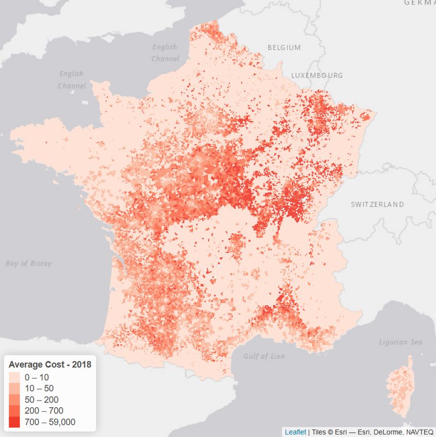
obtained is visible in figure 2b, as at 2018.
(a) Topsoil clay concentration (b) Natural catastrophe occurence
Figure 2: Topsoil clay concentration and historical natural catastrophes ac-
cepted requests. Those two variables will be used for our predictive model.
These variables were then aggregated to the exposure dataset. Thus, the
calibration dataset was composed for each claim year of the “INSEE code” of
the town (from the official classification, that can be seen as the ZIP code used
in the U.S.), the year of the claim, the number of claims, the cost of claims (in
e), the number of policies, the total sums insured (in e), the clay concentration
in the soil, the ESPI, the ESSTI, the ESSWI and Cat (the binary categorical
variable giving the occurrence of a historical natural catastrophe declaration
request, prior to the year of study). All the models calibrated are based on
those five variables mentioned above.
123 Model calibration for the frequency
Using simulations at regional scale, Corti et al. [2009, 2011] pointed out that it is
possible to use simulation to get a good representation of the regions affected by
drought-induced soil subsidence, but substantial differences between simulated
and observed damages in some regions. In this section, we will describe a
simple spatio-temporal model for resilience, to model either the frequency or
the intensity of such events (on a yearly basis). Regression type models will be
considered as in Blauhut et al. [2016]. The main difference is that the interest
was to model occurrence, and a logistic regression was sufficient. Here, since
we focus on frequency and intensity, some Poisson-type regression models will
we considered, first, and then some Gamma models, for the severity, to predict
the economic cost of subsidence. In Section 3.3 we will present regression based
models, that we will extend in Section 3.4 to ensemble models, namely with
bagging of regression trees, as suggested in Breiman [1996] to take into account
some possible non-linearity, as well as cross-effects. And in section 3.5, we will
study more carefully the errors. But before, we need to introduce some criteria
to select an appropriate model.
3.1 Model selection criteria
Various validation performance measures are used to compare the different mod-
els. They are chosen to optimise the model selection based on the qualities that
are desired from the model which are: a good capacity at predicting the correct
number of claims in the right areas, the ability of not predicting claims where
there are none historically all the while keeping the simplest possible model.
The following performance measures are thus used:
• Akaike Information Criteria (AIC) and Bayesian Information Criteria (BIC),
which use maximum likelihood and penalises models with respectively too
many variables and too many variables with respect to the number of
observations. These criteria are only used for the parametric regression
models.
• Root Mean Square Error (RMSE) – or simply the sum of the squares of
errors, which penalises greatly extreme errors, i.e. extreme deviations in
predictions. This will be used for costs, and not counts.
3.2 Cross-Validation method
In order to assess the predictive power of the calibrated models, cross-validation
was used. The main goal of the models is to predict accurately the number of
claims, per town, on a yearly basis, thus a yearly cross-validation, that is derived
from the basic cross-validation principle, will be used.
The idea of cross validation is related to in-sample against out-of-sample
testing. In a nutshell, the model is fitted on a subset of the data, and validation
13is computed on observations that were left out. This approach is interesting to
assess how the results of some statistical analysis will generalize to an ‘indepen-
dent’ data set. Note that it is possible to remove one single observation, and to
validate the model on that one – this is the leave-one-out approach – or to split
the original dataset on k subgroups, to remove one subgroup to fit a model, and
predict on that specific subgroup, and rotate – this is the k-fold cross-validation
approach. In the case of spatio-temporal data,
• use some regions, used as subgroups, then use some spatial k-fold approach
(as in Pohjankukka et al. [2017]) where the model is fitted on k −1 regions,
and validation is based using some metric on the error on the region that
was left out – it can be the sum of the squares of the difference, or any
metric discussed in the previous section,
• use cross-validation in time, but because of particular properties of the
time dimension, cross-validation is performed by removing the future from
the analysis (as in Bergmeir et al. [2018]): at time t, we use observations
up to time t to fit a model, then get a prediction for time t + 1. In some
sense, it is a classical leave-one-out procedure, except that we cannot use
observations after time t + 1 to get a prediction at time t + 1.
3.3 Regression-based models
A first attempt at modelling the yearly number of claims was made using Gen-
eralised Linear Models (GLM) with Poisson, Binomial and Negative Binomial
distributions, which are the most adapted to the calibration data, on counts,
as a starting point. These models offer a simple and interpretable approach
to model data by assuming that the response variable Y = (Yz,t ) ∈ Rn×T is
generated by a given distribution and that its mean is linked to the q explana-
tory variables X = (X z,t ) ∈ X n×T (where classically X = Rq ), through a link
function. In this model, we have n spatial locations (the number of towns), T
dates (the number of years), and q possible explanatory variables.
If we want to model the number of houses claiming a loss in a given location,
the Poisson GLM is defined as Yz,t ∼ P(Ez,t · λz,t ), for a location z and a year
t, where Ez,t is the exposure (the number of contracts in the town) and λz,t is
the yearly intensity, per house,
λz,t = exp [β0 + β1 x1,z,t + · · · + βk xq,z,t ] (4)
where xj,z,t ’s are features used for modeling, such as the ESSWI, the ESSTI, etc.
The prediction, performed at year t + 1 ∈ {2001, ..., 2019} based on a calibration
set of years {2001, ..., t}, is
t Nz,t+1
b = Ex,t+1 · t λ
bx,t+1 (5)
and, based on estimator β b obtained on the training dataset with observations
t
of years {2001, ..., t}, using maximum-likelihood techniques, and
h i
t λz,t+1 = exp β0,t + β1,t x1,z,t+1 + · · · + βk,t xq,z,t+1 (6)
b b b b
14where geophysics covariates xj,z,t+1 are known. In Table 1 several sets of pa-
rameters estimates β
b are given (with t varying from 2008 until 2018).
t
Table 1: Evolution of the parameters in the regression (Poisson regression).
Numbers in brackets are the standard deviations of the parameters. Note that
two ESSPI parameters are not significant here (95% level).
year t 2008 2010 2012 2014 2016 2018
Intercept β0,t
b -13.668 -13.460 -13.522 -13.735 -13.932 -14.357
(0.074) ( 0.071) ( 0.062) ( 0.06) ( 0.059) ( 0.049)
ESSTI βb1,t 1.522 1.420 1.511 1.494 1.539 1.661
(0.017) ( 0.015) ( 0.013) ( 0.013) ( 0.013) ( 0.012)
ESSWI βb2,t -0.711 -0.700 -0.601 -0.709 -0.750 -0.707
(0.011) ( 0.011) ( 0.009) ( 0.009) ( 0.009) ( 0.008)
clay βb3,t 0.021 0.020 0.024 0.025 0.025 0.035
(0.001) ( 0.001) ( 0.001) ( 0.001) ( 0.001) ( 0.001)
cat βb4,t 3.924 3.950 3.957 3.957 4.003 3.902
(0.056) ( 0.055) ( 0.049) ( 0.048) ( 0.047) ( 0.038)
ESSPI βb5,t -0.046 -0.010 0.016 0.074 0.127 -0.048
(0.013) ( 0.011) ( 0.009) ( 0.009) ( 0.009) ( 0.007)
From Table 1, we can see that the model is rather stable over time, which is
an interesting feature from a modeler’s perspective: if we predict more claims
related due to subsidence, it is mainly coming from the underlying factors than
from a change in the impact of each variable. It can be mentioned that βb3,t
(associate the clay) is significantly increasing (with a p-value of 2%).
This Poisson model is rather classical to model counts, and it is said to be an
equi-dispersed model, in the sense that the variance of Y is equal to the average
value. This model can be extended in two directions, instead of having
• the binomial model, where Yz,t ∼ B(Ez,t , pz,t ), where Ez,t is the exposure
and pz,t is the probability that, for a given year t and location z, a claim
is made for a single house, and the prediction for pz,t+1 is
exp βb0,t + βb1,t x1,x,t+1 + · · · + βbk,t xq,x,t+1
tp
bz,t+1 = (7)
1 + exp βb0,t + βb1,t x1,x,t+1 + · · · + βbk,t xq,x,t+1
In that case, we have an under-dispersed model in the sense that, by
construction, we must have Var[Yz,t ] < E[Yz,t ]
• the negative binomial model, where Yz,t ∼ N B(Ez,t , pz,t ), where Ez,t is
the exposure and pz,t is the probability, with standard notations for the
negative binomial probablity function. In that case, we have an over-
dispersed model in the sense that Var[Yz,t ] > E[Yz,t ]
15Calibrating the GLMs and averaging the indicators over the years spanning from
2001 to 2018, using the yearly cross-validation method, the results on the left
of Table 2 were obtained. This table shows that the Negative Binomial model
has the lowest AIC and BIC.
In order to better consider the characteristics of the claims data, Zero-
Inflated models were tested using Poisson and Negative-Binomial distributions.
In these models the joint use of logistic and count regression allows the inte-
gration of the over-representation of non-events in the data. More formally, in
Zero-Inflated models, given a location and a time (z, t), we assume that there
is a probably to have 0 claims. In our context, it could mean that the town has
not been recognized as hit by a drought event. The occurrence of a drought
is modeled with a logistic model, with probability pz,t , here. Then, if there is
a drought event, the number of claims is driven by some specific distribution
(Poisson, Binomial, or Negative Binomial), as introduced by Lambert [1992]. If
we consider some Poisson regression, it means that
P(Yz,t = 0) = pz,t + (1 − pz,t )e−λz,t ·Ez,t (8)
(the second part comes from the fact there there could be a drought, but the
number of counts of claims is null) and
[λz,t · Ez,t ]y e−λz,t ·Ez,t
P(Yz,t = y) = (1 − pz,t ) , where y = 1, 2, 3, · · · (9)
y!
where λz,t and pz,t are related to covariates through expressions as Equation
(4) and (7), respectively. Note that such models can easily be estimated with
standard statistical packages. The results of the Zero-Inflated models are visible
on the right of Table 2. It shows that the Zero-Inflated Negative-Binomial model
is better than the Zero-Inflated Poisson model.
Table 2: Quality measures for the different GLM distributions.
zero-inflated
Binomial Poisson NB Poisson NB
AIC 115,051 114,189 100,491 71,154 54,375
BIC 115,113 114,252 100,564 71,259 54,510
Figure 3 shows the yearly predictions for the zero-inflated models, alongside
the previously tested GLMs3 .
When looking at the yearly total predictions compared to reality, as observed
in figure 3, all the GLM predictions are very similar apart from the negative
binomial model which overpredicts (massively) in 2018, however they all overes-
timate claims in 2018 and underestimating the number of claims in 2003, 2011,
3 For purposes of confidentiality, the total number of claims per year are withheld, but the
proportions on the y-axis are valid.
16Figure 3: Yearly predictions for the Zero-Inflated models and GLMs
2016 and 2017. This graph shows that the predictions closest to the reality
line are for the Negative-Binomial Zero-Inflated model. That model also has
the best metrics when comparing to those of the GLMs. Thus, Zero-Inflated
models appear to provide a better fit than the GLMs.
This section showed that the Zero-Inflated models, in particular the Negative-
Binomial Zero-Inflated model, outperformed the GLMs in terms of number of
claims and model selection criteria. In the next section, we will see of alter-
natives to regression-type models can be considered, since the “linear model ”
assumption might be rather strong here.
3.4 Tree-based models
Tree-based models are popular models for data analysis and prediction and offer
an alternative to the previous parametric models. Popularised by Breiman et al.
[1983], regression trees produce simple and easily interpretable split rules.
• A Regression Tree is such that
L
X
t Yz,t+1 =
b b`,t 1(xz,t+1 ∈ L` )
ω (10)
`=1
where {L1 , · · · , LL } is a partition of X , and Lj ’s are called leaves. In a
tree with two leaves, {L1 , L2 }, there is a variable j such that L1 is the half-
space of X characterized by xj,t ≤ s while L2 is characterized by xj,t > s
for some threshold s. For the “classical” regression tree, the split is based
on the squared loss function, in the sense that we select s to maximise
the between-variance, or equivalently, minimise the within-variance. It
is possible to extend this approach by using, instead of the squares of
residuals (corresponding to the squared loss function), the opposite of
17the log-likelihood of the data. This can be performed using the rpart R
package (see Breiman et al. [1983] for further details on regression trees).
If trees are simple to interprete, they are usually rather unstable: when fitting a
tree on subsets of observation, it is common to get different splitting variables,
and therefore different trees. The idea of bagging (as defined in Breiman [1996])
is to use a boostrap procedure to create samples (resampling the observations
with replacement), and then to aggregate predictions. In the case where the
number of covariates is not too large, this will be also called a Random Forests,
from Breiman [2001].
Some Tree-Based models are tested in order to attempt to improve the pre-
vious predictions. Three tree-based approaches were used, here:
• A “classical” Random Forest (RF),
m L i
1 X b (i) b (i)
X (i) (i)
t Yz,t+1
b = t Yz,t+1 where t Yz,t+1 = b`,t 1(xz,t+1 ∈ L` )
ω (11)
m i=1
`=1
where each tree – corresponding here to different i’s – is computed using a
squared loss function, on different boostrap samples (obtained by resam-
pling n observations, with replacement, out of the initial n ones). This
can be performed using randomForest R package.
• A Poisson Random Forest (RFP) which considers count data, with the aim
to better capture the distribution of the data. Poisson Random Forests
are a modified version of Breiman’s Random Forest allowing the use of
count data with different observation exposures. This is done by modify-
ing the splitting criterion so that it maximised the decrease of the Poisson
deviance and an offset has been introduced to accommodate for differ-
ent exposures. This Random Forest was calibrated using the rfPoisson
function available in the rfCountData package in R.
These Random Forests were all tuned in order to obtain optimal number of
trees, number of variables tested at each split and maximum number of nodes.
However, the tuning was limited given the length of the tuning process, which
may reduce the quality of the models.
The figure 4 shows the total yearly predictions for each tree-based model
alongside the Zero-Inflated Negative Binomial model and the real claims.
Figure 4 shows that the closest predictions to the real observations (the
plain line) seem to be those of the Zero Inflated model and the Poisson Random
Forest, although all models but the Zero-Inflated model underestimates 2011
and 2016. With our cross-validation approach, we have poor results for early
years (only data from 2002 were used to derive a model for 2003). The standard
Random Forest overpredicts 2018.Thus, the Zero-Inflated model and the Poisson
Random Forest appear to have the best predictions.
18Figure 4: Comparison of yearly predictions for the tree-based models, with
ZINB, classical RF, and RFP.
Through this section, two different Random Forests were presented; how-
ever, the one with the best results is the Poisson Random Forest which rendered
similar results to the Negative-Binomial Zero-Inflated model. The complex cali-
bration process and the unclear influence and importance of the variables on the
output of the Poisson Random Forest make it a less attractive choice of model
compared to the Zero-Inflated regression, which has a clear variable influence
and a simple prediction formula. One can thus wonder whether such a loss in
interpretability is worth such a small gain in term of predictions.
3.5 Mapping the predictions
In order to improve the predictions, and only predict the actually impacted
areas, a methodology was developed to optimise the removal of all the very
low claim predictions. This methodology was applied to both the Zero-Inflated
model and the Poisson Random Forest. The total predictions changed little,
and the geographical distribution of both models’ predictions are observable for
2018 in figure 5.
In 2018, both models have more or less the same claim distribution, with
large amounts of claims along the Mediterranean, in the North and in Pays-
de-la-Loire. However, the distribution is slightly different when looking at the
centre of France. Indeed, the Random Forest seems to predict more claims in
that area than the Zero-Inflated Negative Binomial model. Comparing these
results with the real claims for 2018, it can be seen that the historical claims
are nearly exclusively concentrated in the centre of France with a few claims
along the Atlantic and Mediterranean coast and in the North-East of France.
Thus, both models seem to over predict the claims around the coasts of France
and - slightly for the Poisson Random Forest and vastly for the Zero-Inflated
Negative Binomial model - under-predict in the centre of France. However, it
19(a) Poisson RF (b) Zero-Inflated
(c) Observed claims (d) Nat.Cats.
Figure 5: Observed and Predicted number of claims for 2018
can be noted that the over-predicted areas do mostly fall within areas that have
non-recognised natural catastrophe declarations which could mean that the area
was hit but not compensated and thus that the models have difficulty assessing
the difference between areas that will be recognised as natural catastrophes, or
not. The same conclusion can be made when looking at the predictions for 2017,
visible in figure 6.
In these maps, the predicted claims do appear to be in the correct areas in
the South and South-West of France for both models, however, there are over-
predictions in the East, centre and North of France, which also appear to be
areas with non accepted natural catastrophe declarations. Both models seem to
predict the correct areas but also additional zones that often are areas that have
refused natural catastrophe declaration, which means that those areas were im-
20(a) Poisson Random Forrest (RFP) (b) Zero-Inflated (ZINB)
(c) Observed claims (d) Nat.Cats.
Figure 6: Observed and Predicted number of claims for 2017
pacted by subsidence but not sufficiently to enter into the scope of the natural
catastrophe regime. Indeed, as the acceptance criteria changed frequently be-
tween 2001 and 2018, the models cannot capture the natural catastrophe aspect
of a claim seeing as one that may have been acceptable in 2017 may no longer
be today. Both models predict more or less the same geographical distribution
of claims, posing the question of the usefulness and practicality of using a com-
plex model such as the Poisson Random Forest compared to the Zero-Inflated
Negative-Binomial model.
Another option that would permit the classification of the predicted claims
into accepted and refuse natural catastrophe categories, would be to use the
Shrinkage and Swelling of clay risk map Georisques [2020], published by Geo-
logical and mining research bureau (BRGM). This map categorises the exposure
of a given point of France between four categories: not at risk, low risk, aver-
age risk and high risk. The acceptance of a natural catastrophe declaration in
21France is feasible if more than 3% of the surface of a town is in a zone with
average or high risk. Thus, if the predicted claims map and the risk map, ag-
gregated by town, were overlapped, the classification of the predicted claims
would be possible between potentially accepted and most likely refused natural
catastrophe declaration.
4 Cost predictions
In the previous section, we’ve seen different models to predict the frequency
(the number of claims per town), and here, we consider some Gamma model for
average cost per claim, leading us towards a compound model for the total cost
per town, as introduced in Adelson [1966], and used for example in hydrology in
Revfeim [1984] or Svensson et al. [2017], or for droughts in Khaliq et al. [2011].
4.1 Modeling average and total economic costs
For a given location z and year t, the total cost (from the insurer’s perspective)
is a compound sum, in the sense that
Nz,t
(
X Z1,x,t + · · · + ZNz,t ,x,t if Nz,t > 0
Yz,t = Zi,x,t = (12)
i=1
0 if Nz,t = 0,
with a random sum of random costs. Here Nz,t is the frequency, modeled in
the previous section, and Zi,x,t ’s are individual economic losses per house. It
is possible to consider some Tweedie GLM, as introduced in Jørgensen [1997],
corresponding to some compound Poisson model, with Gamma average cost.
Nevertheless this is only a subclass of the general compound models. Note that
Tweedie models are related to some power-parameter, since they are charac-
terize by a relationship E[Y ] = Var[Y ]γ . If γ = 1, Y is proportional to some
Poisson distribution (average costs are non-random) while γ = 2 means that
Y is proportional to some Gamma distribution (frequency is non-random). For
inference, we used γ = 1.5 which corresponds the lowest AIC. For that Tweedie
model, SSTI, SSWI, as well as Clay and Cat covariates were used.
If the model is interesting, it is less flexible than have two separate models,
one for the frequency, and one for the average cost at location z, for year t, and
to write
Yz,t = Nz,t · Z x,t (13)
where (as before) Nz,t is the frequency, as modeled in the previous section, and
we can use our data, aggregated at the town level, to model the average cost
(per house) Z x,t . The prediction is then
t Yz,t+1
b bz,t+1 · t Zbz,t+1
= tN (14)
The results of these methods are rather similar. Figure 7 shows the yearly pre-
dictions for the Tweedie model and the average cost of claims method using the
22GLM and both the Zero-Inflated and Poisson Random Forest models, previously
calibrated.
Figure 7: Yearly cost predictions, with a ZINB model + Gamma costs, RFP
model + Gamma costs, and a Tweedie model (Poisson + Gamma costs).
Figure 7 shows that the Tweedie model makes predictions that are similar to
the previous cost of claims predictions, however this model over-estimates less
the year 2018 and (clearly) over-estimates more the years 2007 and 2012. On
the other hand, the years 2003, 2011 and 2016 are still severely underestimated
by the three predictions, although less so by the Tweedie model.
4.2 Mapping the predictions
As in section 3.5, it is possible to visualize the prediction, and to map 2016 Ybz,2017
and 2017 Ybz,2018 , on Figure 8. As expected, if we are not able to predict correctly
the frequency, the cost is overestimated. Overall (as we can see on Figure 7),
in 2017, we obtained a good prediction, in France, but we can visualize some
spatial differences. Most of the comments made in section 3.5 remain valid, and
clearly, predicted the economics losses in a specific area is not a simple task.
5 Conclusion
The increase in number and severity of subsidence claims in the past years has
created a need for insurers to better grasp their knowledge of this risk. How-
ever, the implementation of subsidence models is time consuming and requires
detailed data. This study proposed a method of approaching the costs and fre-
quency of claims due to subsidence based on historical data. This was applied
through two main components: the development of new drought indicators using
Open Data and the use of parametric and tree-based models to model this risk.
Modelling subsidence requires the integration of meteorological and geological
indicators to ascertain the factors predisposing a policy to subsidence. With-
out this information, the inherent risk to which a dwelling is exposed cannot
23You can also read