Multi-century impacts of ice retreat on sea level and tides in Hudson Bay

Multi-century impacts of ice retreat on sea level and
 tides in Hudson Bay

 Anna-Mireilla Hayden

 Department of Earth and Planetary Sciences

 McGill University

 Montréal, Quebec

 February 2019

A thesis submitted to McGill University in partial fulfillment of the requirements of the degree
 of Master of Science

 © Anna-Mireilla Hayden, 2019

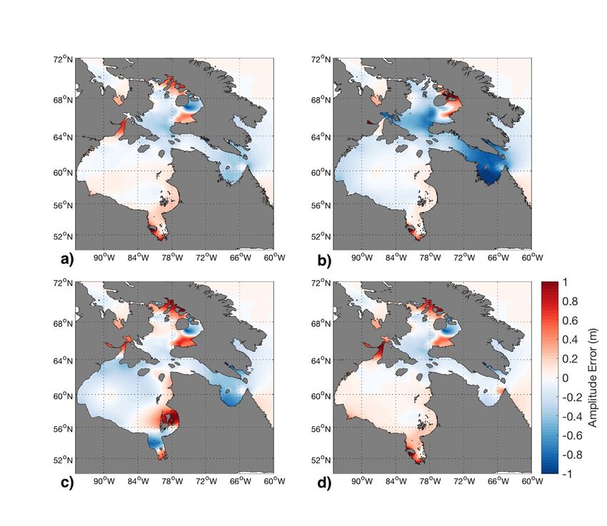
Table of Contents
Table of Contents .......................................................................................................................... 2
Acknowledgements ....................................................................................................................... 3
Contribution of Authors ............................................................................................................... 5
List of Figures ................................................................................................................................ 6
List of Tables ................................................................................................................................. 9
Abstract ........................................................................................................................................ 10
Résumé ......................................................................................................................................... 12
1. Introduction ............................................................................................................................. 14
 1.1 Spatially variable sea level changes............................................................................................... 14
 1.1.2 The sea level model and sea level fingerprints.......................................................................... 16
 1.1.3 Past and present sea level changes in the Hudson Bay ............................................................. 18
 1.1.4 Representative Concentration Pathways ................................................................................... 20
 1.2 Tides ................................................................................................................................................. 22
 1.2.1 Properties of waves and tides .................................................................................................... 22
 1.2.3 Harmonic Constituents .............................................................................................................. 26
 1.2.4 Tide modelling .......................................................................................................................... 29
2. Multi-century impacts of ice sheet retreat on sea level and ocean tides in Hudson Bay .. 31
 2.1 Abstract ........................................................................................................................................... 31
 2.2 Plain Language Summary.............................................................................................................. 32
 2.3 Key Points........................................................................................................................................ 32
 2.4 Introduction .................................................................................................................................... 32
 2.5 Methods ........................................................................................................................................... 36
 2.5.1 Sea level and ice sheet modelling.............................................................................................. 36
 2.5.2 Tide modelling .......................................................................................................................... 38
 2.6 Constraints on modern bathymetry .............................................................................................. 38
 2.7 Results .............................................................................................................................................. 41
 2.7.1 Sea level change ........................................................................................................................ 41
 2.7.2 Tides .......................................................................................................................................... 46
 2.8 Discussion and Conclusions ........................................................................................................... 48
 2.9 Supplementary Figures .................................................................................................................. 53
3. Conclusions and Implications of research ............................................................................ 58
 3.1 Conclusions...................................................................................................................................... 58
 3.2 Future research directions ............................................................................................................. 58
 3.3 Implications of research ................................................................................................................. 59
References .................................................................................................................................... 61

 2

Acknowledgements
 First and foremost, I would like to extend my sincerest thanks to my supervisor, Dr.
Natalya Gomez for her continual support and steadfast encouragement throughout my Master’s.
Natalya’s vast knowledge enkindled my desire to learn more and take action through research.
 Special thanks to my collaborators and colleagues. Among these, I wish to thank
especially Sophie-Berenice Wilmes, Mattias Green, Linda Pan, Holly Han, and Nick Golledge
whose comments and insight helped to shape this thesis. I am thankful for the financial support
for this project provided by NSERC and Québec-Océan.
 I would like to thank all members of the Gomez Geodynamics Group (GGG!), past and
present, for enriching my experience as a graduate student. In particular, thank you to Erik Chan,
Holly Han, Dave Purnell, Linda Pan, and Jeannette Wan, for their companionship and
enthusiasm.
 I would also like to express my deepest appreciation to Dr. Jeffrey McKenzie, who
offered unwavering guidance and valuable advice, especially when graduate school was
particularly “tidal”.
 I am extremely grateful to Dr. William Minarik, who has served as a mentor throughout
my undergraduate and graduate studies.
 I have been privileged to have studied under the supervision of Dr. Bruno Tremblay
during my Master’s. I am thankful for his wisdom, time, and for reassuring me throughout my
studies.
 Anne, Kristy, and Angela: Thank you for all your assistance and hard work in keeping
our department running smoothly.
 I am incredibly grateful for all the love and support from my family: Mom, Angelisa,
Mama, Papa, and Randy – thank you for always believing in me and for providing endless
encouragement throughout my studies.
 Frédéric, thank you for reminding me to stay positive, for your patience and company
while I would work long nights and weekends on this thesis, and for enthusiastically joining me
on any adventure I suggested.
 I dedicate this thesis to my papa, my north star, Dr. John Terry Dennis. I am inspired by
his grit, patience, love, and zest for life. His curiosity in my academic endeavours provided me

 3

with an invaluable outlet for scientific expression, without which I would have not been able to
complete this thesis.

 4

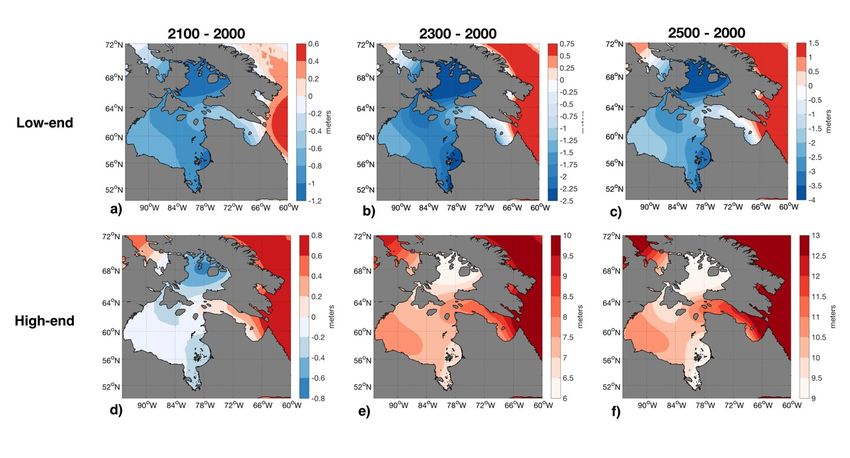
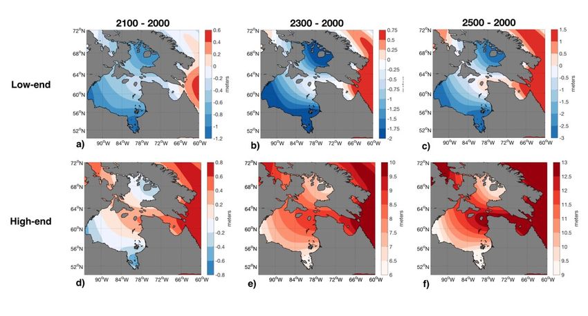
Contribution of Authors
 The following thesis presents original research conducted by the author at the Department
of Earth and Planetary Sciences at McGill University, under the supervision of Dr. Natalya
Gomez. This thesis is presented as a manuscript submitted for publication in the peer-reviewed
Journal of Geophysical Research: Oceans. The author is the primary contributor to the data
analysis and writing and is listed as first author. The manuscript is entitled “Multi-century
impacts of ice sheet retreat on sea level and tides in Hudson Bay” and is co-authored by Natalya
Gomez, Sophie-Berenice Wilmes, Mattias Green, Linda Pan, Holly Han, and Nicholas R.
Golledge. All co-authors have contributed intellectually to the modelling, analysis, interpretation
of data, and writing and proofreading of the manuscript.

 5

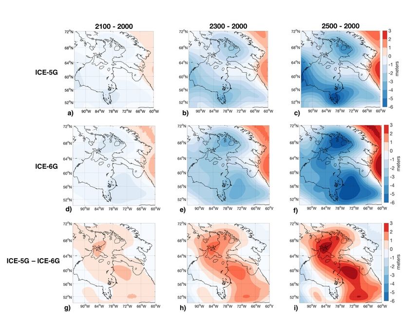
List of Figures
Figure 1: Schematic showing solid Earth deformation during glaciations and interglacials. a)
Solid Earth subsidence and rebound due to ice loading during glacial periods. The solid Earth
below the ice sheet is depressed and the mantle flows downwards and spreads out laterally. At
the peripheral regions, called forebulges, the land rises. b) Solid Earth subsidence and rebound
due to ice loading during interglacial periods. The solid Earth below the former ice sheet rises
and the forebulges collapse. Figure from Tom James, Natural Resources Canada. ..................... 19
Figure 2: Relative sea level changes at Churchill, Manitoba. The black points show the
measurements from the tide gauge station at Churchill, with the blue curve connecting the points,
the red line indicates the mean trend. This figure illustrates the relative sea level fall through time
as a response to vertical land motion due to past ice loading changes. Data from the Permanent
Service for Mean Sea Level (PSMSL).......................................................................................... 20
Figure 3: Terminology used to describe waves. Sinusoidal wave form as seen a) in space from
an instant in time and b) at a fixed location over an interval in time. Figure from Forrester
(1983). ........................................................................................................................................... 23
Figure 4: Diagram to show positions in the Earth–Moon system that are used to derive the tidal
forces. The separation is distorted but the relative diameters of the Earth and Moon are to scale.
Figure from Pugh & Woodworth (2014). ..................................................................................... 25
Figure 5: Spring–neap tidal cycles are produced by the relative motions of the Moon and Sun, at
14.8-day intervals. a) Spring tides occur at new and full moon, b) neap tides occur at the Moon’s
first and last quarter. Figure from Pugh & Woodworth (2014). ................................................... 28
Figure 6: a) Bathymetry and topography of the Hudson Bay Complex, defined here as Hudson
Bay, James Bay, Foxe Basin and Hudson Strait, b) Present day semi-diurnal (M2) tidal
amplitudes (colour) and phases (contoured in white lines at 1/8 M2 period), taken from the
TPXO8 tide database (http://volkov.oce.orst.edu/tides/tpxo8_atlas.html). .................................. 34
Figure 7: Amplitude error between simulated M2 amplitudes from several bathymetry datasets
and observed M2 amplitudes from TPXO8. a) GEBCO 2014 (Weatherall et al., 2015), b)
SRTM30_Plus (Becker et al., 2009), c) GEBCO 2008 (http://www.gebco.net), d) our new,
composite bathymetry with SRTM30_Plus in Hudson Bay and GEBCO 2008 elsewhere. ......... 40
Figure 8: Contributions to sea level change in the HBC from GIA and future melting of the polar
ice sheets under RCP8.5 at 2100, 2300 and 2500, relative to 2000. Blue shading corresponds to a

 6

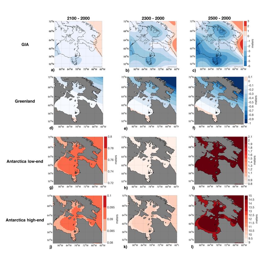
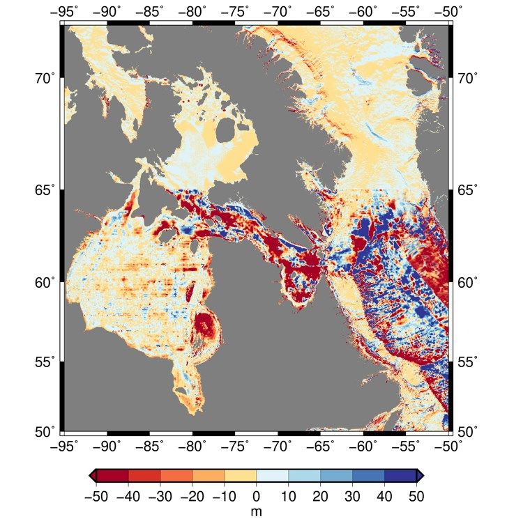
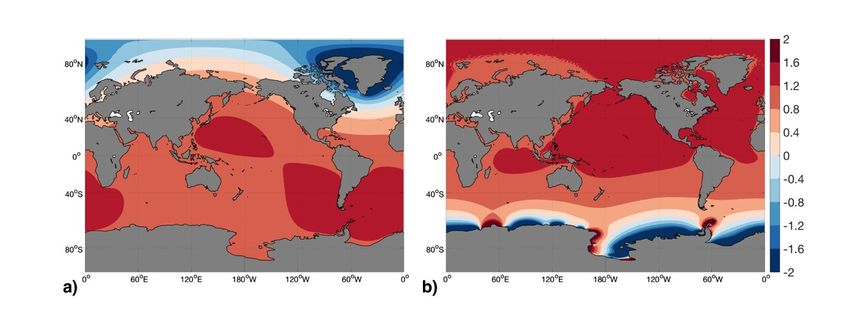
sea level fall and red shading corresponds to a sea level rise. (a-c) Contribution to sea level
change from past ice-ocean loading changes (i.e. GIA) over the last deglaciation associated with
the ICE-5G ice history (Peltier, 2004). (d-f) Contribution to sea level change from the Greenland
Ice Sheet (Golledge et al., 2019. (g-l) Contribution to sea level change from the Antarctic Ice
Sheet under from (g-i) low-end (Golledge et al., 2019) and (j-l) high-end (Pollard et al., 2017)
projections. Note the different color scales used for the 2100, and the 2300 and 2500 projections
in panels g-l. .................................................................................................................................. 44
Figure 9: Total projected sea level change at 2100, 2300, and 2500, relative to 2000. Sum of
individual contributions presented in Figure 8. Panels a-c correspond to the low-end Antarctic
ice loss scenario (Golledge et al., 2019). Panels d-f correspond to the high-end Antarctic ice loss
scenario (Pollard et al., 2017). ...................................................................................................... 45
Figure S1: Contribution of glacial isostatic adjustment (GIA) to sea level changes in the Hudson
Bay Complex at 2100, 2300, and 2500 relative to 2000 adopting ICE-5G (Peltier, 2004) (a-c) and
ICE-6G (Argus et al., 2014; Peltier et al., 2015) (d-f) ice histories. Panels g-i represent the
difference between panels a-c and d-f. Note that in the main manuscript, we adopt the ICE-5G
ice history as the spatial pattern of ice loading and unloading in ICE-6G in this region is
unrealistic. ..................................................................................................................................... 53
Figure S2: Difference between the GEBCO 2014 and ETOPO bathymetry datasets. Differences
are saturated beyond ± 50 meters, but exceed 200 meters in parts of Hudson Strait. .................. 54
Figure S3: Normalized fingerprint of sea level change associated with melting of a) the
Greenland Ice Sheet and b) the Antarctic Ice Sheet. Normalized fingerprints are calculated by
dividing the spatially variable sea level change by the eustatic equivalent value (EEV, or global
average) of sea level change associated with the ice loss. ............................................................ 54
Figure S4: Total projected sea level change at 2100, 2300, and 2500, relative to 2000, adopting
the ICE6-G ice history (Argus et al., 2014; Peltier et al., 2015). Sum of individual contributions
presented in Figure 8. Panels a-c correspond to the low-end Antarctic ice loss scenario
(Golledge et al., 2019). Panels d-f correspond to the high-end Antarctic ice loss scenario (Pollard
et al., 2017). .................................................................................................................................. 55
Figure S5: Total projected a) sea level and b) tidal amplitude changes at 2200, relative to 2000,
incorporating the contributions of Greenland ice loss, GIA, and the high-end Antarctic ice loss
scenario. ........................................................................................................................................ 55

 7

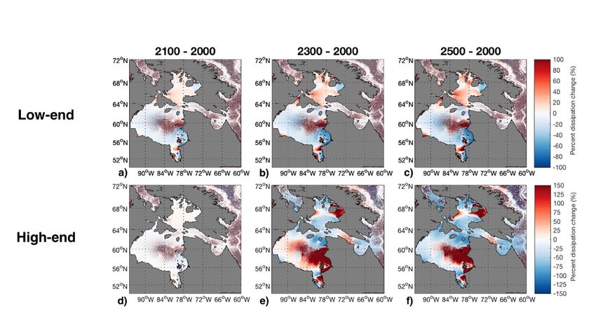
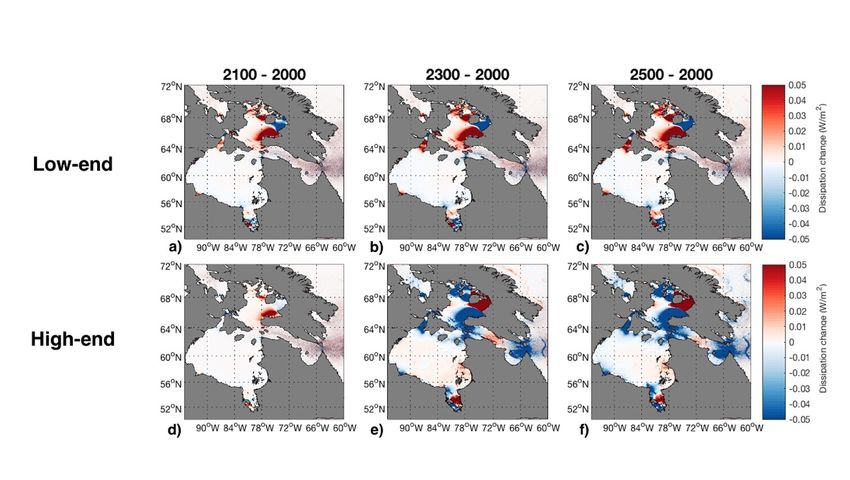
Figure S6: Sea level (a-c) and M2 tidal amplitude (d-f) changes associated with Greenland ice
loss at 2100, 2300 and 2500, relative to 2000............................................................................... 56
Figure S7: M2 tidal energy dissipation change at 2100, 2300, and 2500, relative to 2000 under
our low-end (a-c) and high-end (d-f) Antarctic ice loss scenarios................................................ 56
Figure S8: Percent M2 tidal energy dissipation change at 2100, 2300, and 2500, relative to 2000
under our low-end (a-c) and high-end (d-f) Antarctic ice loss scenarios. .................................... 57

 8

List of Tables
Table 1: Total (all water depths) and deep ocean (water depths > 500 m) root mean square error
between predicted M2 amplitudes from several bathymetry datasets and observed M2 amplitudes
from TPXO8. ................................................................................................................................ 41

 9

Abstract
 Sea level change associated with ongoing and future melting of the Greenland and
Antarctic Ice Sheets is one of the most threatening consequences of anthropogenic climate
change and will greatly impact low-lying coastal communities. Regional sea level changes
associated with changes in grounded ice mass can differ significantly from the globally averaged
value due to gravitational, rotational, and Earth deformational effects. In addition to
contemporary changes in the current polar ice sheets, past changes in ice sheet configurations
over the last glacial cycle also contribute significantly to regional trends in sea level. This is
especially true in the case of Hudson Bay, a shallow inland sea in northern Canada that was ice
covered at the Last Glacial Maximum leading to ongoing crustal uplift and sea level fall of up to
1cm/year in the modern. It remains to be seen whether this trend will continue in the coming
centuries as the polar ice sheets retreat because it is unclear what the dominant contributor to sea
level change in the Hudson Bay will be, or even what the sign will be. Sea level changes in turn
affect tidal dynamics due to the sensitivity of tides to water depth, and recent work has suggested
that future sea level changes as a consequence of ice sheet collapse will impact tides globally.
However, previous studies on both modern and future tides have been unable to accurately
model tides in Hudson Bay due to large uncertainties in bathymetry in the bay.
 This thesis addresses the aforementioned knowledge gaps and quantifies the impact of
past and future ice sheet retreat on sea level and tides in the Hudson Bay region. In Chapter 1, I
outline the background theory on sea level and tides. In Chapter 2, I present a paper, submitted to
Journal of Geophysical Research: Oceans, in which coauthors and I model sea level changes
over the next 500 years associated with the combined effects of ongoing glacial isostatic
adjustment and future ice loss from the Greenland and Antarctic Ice Sheets and the resulting
changes in ocean tides in Hudson Bay. To establish an initial condition for the simulations, we
investigate the accuracy of current bathymetry datasets in reproducing modern ocean tides
measured from satellite observations. We produce a new, improved bathymetry dataset in the
bay constrained, for the first time, using tide observations. It is shown that the Antarctic ice loss
scenario considered determines the sign and magnitude of sea level and tide changes in the
Hudson Bay region, with the largest changes projected in the adjacent Hudson Strait.
Furthermore, it is demonstrated that future sea level rise would greatly affect tidal energy
dissipation in the region, which could have significant and widespread impacts on the global

 10

tidal energy balance. Chapter 3 concludes this thesis with a discussion and recommendations for
future directions of research and the consequences of our results on navigation, ecosystems, and
societies.

 11

Résumé
 Les variations du niveau de la mer, causées par la fonte actuelle et future des inlandsis au
Groenland et en Antarctique, sont l’une des conséquences les plus graves des changements
climatiques anthropiques, et auront un impact considérable sur les communautés de basses-terres
côtières. Les variations régionales du niveau de la mer, associées aux changements dans la masse
des glaces ancrées, peuvent significativement différer de la valeur moyenne globale en raison des
effets gravitationnels, rotationnels, et de la déformation de la Terre. En plus des changements
actuels concernant les inlandsis polaires, les transformations passées au sujet des configurations
des inlandsis lors de la période glaciaire précédente, ont aussi significativement contribuées aux
variabilités régionales du niveau de la mer. Ceci est particulièrement vrai dans le cas de la Baie
d’Hudson, une mer intérieure peu profonde au nord du Canada qui était recouverte de glace
pendant le dernier maximum glaciaire, entrainant un rebond post-glaciaire continu et une baisse
du niveau de la mer jusqu’à 1cm/an actuellement. Il reste à voir si cette tendance se poursuivra
au cours des prochains siècles alors que les inlandsis polaires se retirent. Ainsi, il n’est pas
clairement établi quel sera le principal facteur de variation du niveau de la mer dans la Baie
d’Hudson, ni même quel sera le signe. Les variations du niveau de la mer ont à leur tour une
incidence sur la dynamique des marées en raison de la sensibilité des marées par rapport à la
profondeur d’eau; une étude récente a suggéré que les variations futures du niveau de la mer,
résultant de l’effondrement des inlandsis, auront un impact sur les marées à l’échelle mondiale.
Cependant, des études antérieures sur les marées présentes et futures n’ont pas permis de
modéliser avec exactitude les marées dans la Baie d’Hudson, et cela en raison des grandes
incertitudes entourant la bathymétrie de la baie.
 Cette thèse aborde les manques de connaissances susmentionnés et quantifie l’impact du
recul des inlandsis passés et futurs sur le niveau de la mer et les marées de la région de la Baie
d’Hudson. Le chapitre 1 présente le contexte théorique sur le niveau de la mer et des marées. Le
chapitre 2 présente un article soumis au Journal of Geophysical Research: Oceans, dans lequel
les co-auteurs et moi-même modélisons les variations du niveau de la mer au cours des 500
prochaines années qui sont associées à l’effet combiné d’ajustement glaciaire isostatique en
cours et à la future perte de glace des inlandsis du Groenland et de l’Antarctique, ainsi que les
changements qui en découlent concernant les marées de la Baie d’Hudson. Afin d’établir une
condition initiale pour des simulations, nous examinons l’exactitude des données actuelles de

 12

bathymétrie en reproduisant les marées océaniques actuelles mesurées à partir d’observations
satellites. Nous produisons un nouvel ensemble de données bathymétriques amélioré, contraint
pour la première fois en utilisant les observations des marées. Il est démontré que le scénario
considéré de perte de glace en Antarctique détermine le signe et la magnitude des variations du
niveau de la mer et des marées dans la région de la Baie d’Hudson, les plus importantes étant
projetées dans le Détroit d’Hudson adjacent. De plus, il est démontré que la hausse future du
niveau de la mer aurait une incidence importante sur la dissipation de l’énergie des marées dans
la région, ce qui pourrait avoir des effets importants et répandus sur l’équilibre mondial de
l’énergie des marées. Le chapitre 3 conclut cette thèse avec une discussion et des
recommandations sur les orientations futures de recherche et les conséquences de nos résultats
sur la navigation, les écosystèmes et les sociétés.

 13

1. Introduction

1.1 Spatially variable sea level changes
 Sea level changes occur over a large range of temporal scales, from sub-daily (e.g. tides)
to millions of years (e.g. mantle convection). In the coming centuries, future global mean sea
level changes are expected to be dominated by contributions from the Greenland and Antarctic
Ice Sheets (Church et al., 2013). However, the resulting pattern of sea level change associated
with melting ice sheets is far from uniform and exhibits significant geographical variability
(Clark & Lingle, 1977; Gomez et al., 2010; Mitrovica et al., 2001; Woodward, 1888). To
appreciate and understand why such patterns emerge, this section begins with a discussion on the
physics of sea level change associated with surface mass (ice and water) loading redistribution.
Next, I present an overview of sea level changes in Hudson Bay. This section concludes with a
discussion of the Representative Concentration Pathway framework for predicting future sea
level change.

1.1.1 Sea level theory
 In this section, I describe the sea level equation that includes migrating shorelines, Earth
rotation and deformation of the solid Earth. A complete derivation of the sea level equation is
available in Gomez et al. (2010) and Mitrovica et al. (2011).
 It is first necessary to define the usage of relative sea level ( ). Relative sea level is
defined as the difference between the height of the ocean surface equipotential, or geoid, , and
the solid earth surface, , at a specific colatitude ( ) and colongitude ( ) at time :

 ( , , ) = ( , , ) − ( , , ) (1)

 The total change in the globally defined sea level at time can be calculated as:

 ( , , ) = ( , , ) − ( , , ) (2)

 14

 is defined at every location on the globe. Topography ( ) is then defined as the
negative of relative sea level ( ), i.e. the elevation of the land is negative sea level:

 ( ) = − ( ) (3)

 Conversely, ocean height ( ) is only defined over the oceans. To obtain , is projected
onto the ocean function, ∗ , which defines the regions where oceans are present:

 1, > 0 ℎ 
 ∗ = { (4)
 0, ℎ 

 With these terms defined, we can introduce the sea level equation that accounts for
shoreline migration. For a given location and time , the change in ocean height Δ is defined as
the change in sea level (Δ ) projected onto the ocean function minus the topography 
projected onto the change in the ocean function:

 Δ ( , , ) = Δ ( , , ) ∗ ∗ ( , , ) − ( , , 0 )[ ∗ ( ) − ∗ ( 0 )] (5)

 The first term, Δ ( , , ) ∗ ∗ ( , , ) describes the change in the ocean depth. The
term ( , , 0 )[ ∗ ( ) − ∗ ( 0 )] accounts for shoreline migration. Here, the shoreline is
defined at the location where sea level and topography are equal to each other, such that both
topography and sea level equal 0. Shoreline migration refers to the lateral movement of the ocean
boundary, and can be landwards as sea level rises, or oceanwards as sea level falls.
 ∆Φ
 The term of Δ can be further decomposed into uniform shift (hereafter , where
 
∆Φ is the perturbation to the equipotential and is the acceleration due to gravity) and
geographically variable (hereafter ∆ ) components. The uniform shift component describes the
change in the height of the equipotential on which the ocean surface lies, such that the ocean
surface at a later time lies on a different equipotential compared to = 0. The uniform shift
component is calculated by applying the principle of conservation of mass (i.e. a decrease in ice
sheet mass will result in an increase in ocean mass). The interpretation of the uniform shift in

 15

equipotential is as follows: while the sea surface is assumed to be constrained to an equipotential
surface, over time, the location of this equipotential surface can change as mass is exchanged
between the ice sheets and the oceans. ∆ describes the perturbation to the uniform shift that
arises because of the changes in the gravitational attraction between ice and oceans. Δ can then
be written as:
 ∆Φ 
 Δ ( , , ) = ∆ ( , , ) + (6)
 
 and Δ :
 ∆Φ 
 Δ ( , , ) = Δ ℒ( , , ) + (7)
 
where Δ ℒ is the geographically variable component of . Changes in ∆ ℒ are a function of
changes in grounded ice (ΔI) and ocean height (ΔS), in addition to changes in the angular
velocity of Earth (Δω). Redistributing the mass of the ice sheets and oceans changes the
equipotential on which the ocean height ( ) lies, and this redistribution deforms the planet, which
feeds back into changes in the ocean surface equipotential. With the geographical dependency
implicitly present, the generalized sea level equation can be succinctly written as (see Gomez et
al., 2010 and Mitrovica et al., 2011, for intermediate steps):

 ∆Φ( )
 Δ ( ) = [∆ ℒ(ΔI, ΔS, Δω, ) + ] ∗ ∗ ( ) − ( 0 )[ ∗ ( ) − ∗ ( 0 )] (8)
 
1.1.2 The sea level model and sea level fingerprints
 When an ice sheet melts, sea level does not rise uniformly across the globe. Regional sea
level changes can differ substantially from the global mean sea level change, producing distinct
patterns or “fingerprints” of sea level rise and fall (e.g., Mitrovica et al., 2011). These deviations
are due to spatial variability in gravitational, solid Earth deformational, and Earth rotational
effects, in addition to changes in ocean dynamics. The following section describes the first three
of these effects, as they are included in the sea level model used in this thesis.
 Ice sheets are large enough to exert a gravitational attraction on the water surrounding
them. When ice mass accumulates, there is an increased gravitational attraction exerted by the

 16

ice, causing sea level to rise close to the location of increased mass, while further away sea level
falls. Conversely, when ice mass is lost, the weakened gravitational attraction next to the ice
sheet results in a local sea level fall. At greater distances from the source of ice loss, the sea level
rise is higher than the global average, such that mass is conserved (Tamisiea & Mitrovica, 2011).
 The solid Earth is not completely rigid and yields to mass that is added to its surface, this
effect is known as the Earth deformational effect (Gomez et al., 2010; Mitrovica et al., 2009;
Tamisiea & Mitrovica, 2011). In terms of ice sheets and sea level, this is commonly referred to
as ice and ocean loading. An increase in the mass of the ice load depresses the solid Earth below.
In response to a loss of ice mass, the solid Earth underlying the former ice load begins to
rebound, seeking equilibrium. The solid Earth responds elastically on short timescales, that is,
the land under and adjacent to the waning ice sheet responds instantaneously once the ice load is
removed, and the land rises relative to the ocean. The elastic response to loading changes is
important when considering present day ice loss. Furthermore, the Earth has a memory of the
removal of ice sheets, resulting in the viscous response of the solid Earth over glacial timescales.
Thus, the solid Earth must be modeled as a viscoelastic body when considering the effects of ice
loss on sea level.
 The redistribution of mass also affects the orientation of the Earth’s rotation axis relative
to the Earth’s surface geography, this effect is known as true polar wander (TPW) (Milne &
Mitrovica, 1998; Mitrovica & Milne, 2003; Kendall et al., 2005). With ice sheet growth, the
rotation axis will move away from the ice load in order to conserve angular momentum.
Conversely, when an ice sheet melts, the redistribution of mass orients the rotation axis towards
where the load once was (Gomez et al., 2010). The perturbation in the rotation axis results in two
quadrants of the Earth experiencing an accentuated sea level rise, and two quadrants
experiencing a sea level fall (Gomez et al., 2010; Mitrovica et al., 2009). For Greenland ice loss,
this translates to a large sea level rise in the South Atlantic and Northwest Pacific (Tamisiea &
Mitrovica, 2011). Under West Antarctic melting, the rotational feedback results in an
accentuated sea level rise along the coasts of North America and in the Indian Ocean (Gomez et
al., 2010; Mitrovica et al., 2009; Mitrovica & Tamisiea, 2011).

 17

1.1.3 Past and present sea level changes in the Hudson Bay
 During the Pleistocene epoch, defined here as 2,600,000 – 11,700 years before present
(yr B.P.), changes in the Earth’s climate between colder and warmer periods lead to the growth
and decline, respectively, of continental-sized ice sheets. When the climate is cooler (warmer),
the climate is in a glacial (interglacial) period, and there is more (less) water stored in continental
ice sheets and global sea levels are lower (higher). During the Last Glacial Maximum (LGM,
21,000 – 18,000 yr B.P.), sea levels were 120-130 m lower than present day (Clark et al., 2009),
with two ice sheets covering northern Canada: the Laurentide Ice Sheet and the Innutian Ice
Sheet (Dyke, 2004). At the Laurentide Ice Sheet’s maximum extent, ice 3-4 km thick covered the
Hudson Bay region (Simon et al., 2016). Beneath the ice sheet and within the Earth’s interior,
hot mantle rock flowed downward and spread out laterally, resulting in depression of the Earth’s
crust. At the periphery of the ice sheet, the land rose in response to the outwardly flowing mantle
material (Figure 1a).
 Throughout the early Holocene (9,000 – 6,000 yr B.P.), radiocarbon dates indicate that
the Laurentide Ice Sheet was retreating extensively (Dyke, 2004). By ~ 7,000 yr B.P., the
Laurentide Ice Sheet had melted (Denton et al., 2010) and the process of subsiding and rising
land reversed itself (Figure 1b). Land under the former ice sheet began to rise, and the peripheral
regions began to subside. The influx of meltwater from the rapid retreat of the ice flooded the
surrounding land beyond the current shorelines of present-day Hudson Bay, creating the Tyrrell
Sea (~7,000 yr B.P.; Lee, 1960). As the land continued to rise, the Tyrell Sea drained to form the
present Hudson Bay and James Bay.

 18

Figure 1: Schematic showing solid Earth deformation during glaciations and interglacials. a)
Solid Earth subsidence and rebound due to ice loading during glacial periods. The solid Earth
below the ice sheet is depressed and the mantle flows downwards and spreads out laterally. At
the peripheral regions, called forebulges, the land rises. b) Solid Earth subsidence and rebound
due to ice loading during interglacial periods. The solid Earth below the former ice sheet rises
and the forebulges collapse. Figure from Tom James, Natural Resources Canada.

 The sequence of past ice-ocean mass exchanges yields an ongoing response of the solid
earth to such loading changes, referred to as Glacial Isostatic Adjustment (GIA). This process is
still occurring because the Earth’s mantle behaves like a highly viscous fluid over long time
scales. Therefore, all modern observations of sea level related quantities are impacted by past ice
and ocean loading changes. In Hudson Bay, the rate of glacial isostatic uplift of the land is
approximately 1 cm/year (Peltier, 1999). It follows that the tide gauge in Churchill, Manitoba, is
also detecting the change in the relative sea level, as indicated by a relative long-term sea level
fall (Figure 2).

 19

Figure 2: Relative sea level changes at Churchill, Manitoba. The black points show the
measurements from the tide gauge station at Churchill, with the blue curve connecting the points,
the red line indicates the mean trend. This figure illustrates the relative sea level fall through time
as a response to vertical land motion due to past ice loading changes. Data from the Permanent
Service for Mean Sea Level (PSMSL).

1.1.4 Representative Concentration Pathways
 A growing body of evidence suggests that mass loss from the Greenland and Antarctic
Ice Sheets has accelerated in recent decades (e.g. Chen et al., 2017; Forsberg et al., 2017), and in
the coming centuries the polar ice sheets are expected to dominate sea level change (Church et
al., 2013; Golledge et al., 2015, 2019). Since placing a bound on the future sea level rise due to
ice loss is not a trivial task, it is beneficial to introduce a framework on which sea level
projections are often based. In this section, I describe the Representative Concentration
Pathways, as they guide in the simulations presented in Chapter 2.
 Representative Concentration Pathways (RCPs), formulated by the Intergovernmental
Panel on Climate Change (IPCC) (Moss et al., 2008; 2010), have served as the primary resource
for climate change, and hence, sea level projections in recent years. Four RCPs indicate possible
trajectories of future greenhouse gas concentrations and the associated increase in global mean
surface temperature. On the low end of the spectrum, RCP2.6 assumes a peak in emissions by
2020, followed by a concerted effort to decrease emissions (Meinshausen et al., 2011; Moss et
al., 2008; 2010). Under RCP2.6, the likely increase in global mean temperature by the end of the
century is 1.9-2.3°C above pre-industrial (1850-1900) levels (Meinshausen et al., 2011; Moss et

 20

al., 2008; 2010). Conversely, the emission-intensive RCP8.5 scenario represents steadily
increasing greenhouse gas emissions throughout the twenty-first century, with an accompanying
global mean temperature increase of 3.2-5.4°C above pre-industrial levels (Meinshausen et al.,
2011; Moss et al., 2008; 2010).
 While RCP scenarios presented in the IPCC’s Fifth Assessment Report extend to 2100,
the inertia of the climate system implies a multi-century, and possibly a multi-millennial
commitment to climate change (Clark et al., 2016; DeConto & Pollard, 2016; Golledge et al.,
2015, 2019). Extended Concentration Pathways (ECPs) were developed as a way to project the
changes in greenhouse gas emissions until 2300 (Meinshausen et al., 2011). The framework for
creating an ECP is based on the following three options, as per Meinshausen et al. (2011): 1)
radiative forcing and concentration of greenhouse gas can be kept constant, 2) emissions can be
reduced over time, 3) emissions can continue at a constant rate over time. For instance, in the
emission-intensive RCP8.5, the corresponding ECP8.5 assumes constant emissions until 2150,
followed by a smooth transition to stable concentrations after 2250 (Meinshausen et al., 2011,
Table 3). However, Meinshausen et al. (2011) emphasize that ECPs are highly speculative. To
that end, ECPs should not be interpreted as the definitive pathway that would succeed the
corresponding RCP scenario. Rather, ECPs provide a range of concentrations and forcing
pathways that can be used in climate models, and evolves as does our understanding of earth
system processes and behaviours.
 Greenland’s contribution to sea level change is predominantly driven by surface mass
balance, followed by ice discharge via icebergs (Church et al., 2013). Conversely, the dynamic
response is expected to dominate sea level changes due to Antarctic ice loss, but the future
contribution from Antarctica remain highly uncertain due to the lack of observations to constrain
models and an incomplete description of ice sheet-ocean-atmosphere interactions in current
models (Kopp et al. 2017; Moore et al., 2013; Wingham et al., 2009). As the processes
responsible for ice loss from Greenland are more well understood than those for Antarctica, there
is more agreement in the literature on Greenland’s response to RCP scenarios, which fall within
a likely range of 0.07-0.21 m of globally averaged sea level rise by 2100 in response to RCP8.5
(Church et al., 2013; Clark et al., 2015; Slangen et al., 2016). For Antarctica, estimates range
from 0.1 m to 1.46 m of globally averaged sea level rise by the end of the current century under
the RCP8.5 scenario (Golledge et al., 2015, 2019; Kopp et al., 2017). Recent work by Edwards et

 21

al. (2019) suggests that the highest end Antarctic scenarios are less likely by 2100, but cannot be
ruled out in the longer-term future. Despite the uncertainty, it is agreed upon that the amount of
mass lost from Antarctica and the accompanying sea level change is highly dependent on the
emission scenario (DeConto & Pollard, 2016; Kopp et al., 2017).

1.2 Tides
 Tides are responsible for the daily, short term variability in sea level, with the daily rise
and fall in water levels due to the gravitational attraction of the moon and sun. To place the
current work in context, this section presents an introduction to the theory behind tides. I first
discuss the properties of waves and tides. I then present an overview of the forces causing the
tides, followed by a description of periodic tidal constituents. This section concludes with a
discussion on tide modelling. Current knowledge of tides in Hudson Bay is discussed in detail in
Chapter 2.

1.2.1 Properties of waves and tides
 As tides are a form of wave, it is first necessary to discuss the properties that define a
wave. There are three main properties that define a wave. Firstly, waves do not transport matter,
only energy. Secondly, this energy is transferred through the medium the wave is travelling
through. Therefore, water waves result in the transfer of energy through the medium of water but
not the transfer of water itself. Thirdly, to prevent matter from being displaced, there must be a
resisting force. For tide waves, gravity provides the restoring force through hydrostatic pressure.
 Figure 3 illustrates the main features of a wave: wave crest, wave trough, amplitude,
range, wavelength, period, and frequency. The crest of a wave is the highest point of the wave. In
tidal studies, the crest is referred to as high water (HW). Conversely, the trough is the lowest
point of the wave, and is referred to as low water (LW) in tidal studies. Tidal amplitude refers to
the vertical distance from the equilibrium point of the wave (mean water level, MWL, for tidal
studies) to either the crest or the trough, whereas tidal range measures the distance between the
trough and the crest. The wavelength (λ) is the horizontal distance between two successive crests
or troughs. Tidal period refers to the time elapsed between two successive wave crests or

 22

troughs. The frequency of a wave is defined as the number of periods per unit time. For tides, the
frequency is often expressed as angular speed, measured in degrees per hour.

Figure 3: Terminology used to describe waves. Sinusoidal wave form as seen a) in space from
an instant in time and b) at a fixed location over an interval in time. Figure from Forrester
(1983).

 Waves represent oscillations and can be either free or forced. Free oscillation means that
there is no external force driving the back-and-forth motion, this is the natural frequency of the
wave. Forced oscillations are those in which an external force plays a role in their generation.
Tides are a type of forced oscillations, with the external force provided by the sun and moon’s
unbalanced gravitational attraction force.
 A special form of oscillation in an ocean basin is that of ocean resonance. Resonance
refers to the condition in which the driving and restoring forces within the system are mainly in
unison, with the forcing frequency close to that of the natural frequency of the system. This
produces a large amplitude response. Oscillations in the Bay of Fundy in New Brunswick and
Ungava Bay in northern Quebec are close to resonance with the semi-diurnal M2 tide (Forrester,
1983; Pugh & Woodworth, 2014). Resonance is dependent on the water depth, , and the
length, , of the ocean basin. As represented in Equation 9, a long and/or shallow basin will have

 23

a large natural period (T) of oscillation. However, this equation omits frictional effects, which
becomes important in shallower water.

 2 
 = 1 (9)
 ( )2

1.2.2 The tide generating forces
 Tides are the ocean’s response to the unbalanced gravitational attraction forces of the sun
and moon. It is this unbalanced component of this force that results in the periodic rise and fall of
water levels. Gravitational attraction between two bodies is represented by the Newton’s Law of
Gravitation. This law states that the net gravitational attraction force, , separating two bodies is
proportional to the product of the two masses and inversely proportional to the square of the
distance separating the two bodies. Between the earth and moon, this can be written as:

 = (10)
 2

 Where me is the earth’s mass, ml is the moon’s mass, is the distance separating the two
bodies center of mass, and G is the universal gravitational constant. Similarly, the gravitational
attraction between the sun and earth can be obtained if instead the sun’s mass and earth-sun
center of mass distance is used.
 The tide-generating force of the sun or of the moon is calculated as the difference
between the gravitational attraction at their respective centres of mass and a point of interest on
the earth’s surface. Figure 4 illustrates the lunar tide generating force.

 24

Figure 4: Diagram to show positions in the Earth–Moon system that are used to derive the tidal
forces. The separation is distorted but the relative diameters of the Earth and Moon are to scale.
Figure from Pugh & Woodworth (2014).

 At a point on the earth facing away from the moon in the moon-earth system (P2 in
Figure 4), the gravitational attraction is smaller at this point than at the center of mass and water
moves away from the moon. Mathematically, this is represented by:

 = (11)
 ( + )2

where is the radius of the earth and all other values are as previously defined. At a point on the
earth facing the moon (P1 in Figure 4), the strength of the gravitational force is stronger than at
the center of mass, and the water is pulled towards the moon. This can be shown as:

 = (12)
 ( − )2

 Although the sun’s mass is much greater than that of the moon, and hence has a larger
gravitational pull on the earth, the tide generating force of the moon is approximately two times
stronger than that of the sun. The tide generating force (Ft) varies inversely with the cube of the
distance separating the two bodies, rather than the inverse square. The derivation for the earth-
moon system at a point P1 is presented here:

 25

 
 = − (13)
 ( − )2 2

 which can then be expanded to:

 2 − 2
 = (14)
 4 − 2 3 + 2 2

 Since ≫ , the expression can be simplified and rewritten as:

 2 
 = (15)
 3

 At P2, the tide generating force can be written as:

 2 
 = − (16)
 3

 The net effect of the tide generating force produces two bulges, one on the side of the
earth facing the moon, and the other on the side of the earth opposite the moon.

1.2.3 Harmonic Constituents
 The precisely determined motions of the earth, sun, and moon and their frequencies
enable tides to be analyzed and predicted with great certainty, as the tides are a consequence of
these periodic motions. The description of tides can be decomposed mathematically into
harmonic constituents based on the periodic fluctuations in the tide or tide raising force at a
particular frequency.
 An important distinction must be made regarding the day length and tidal period
conventions. A solar day is 24 hours, and a lunar day is 24 hours and 50 minutes. The day
lengths differ due to different reference points for measuring a complete rotation of the earth. A
solar day represents the complete rotation of the earth with respect to the sun. A lunar day is a
complete rotation of the earth with respect to the moon, it is longer than the solar day because by

 26

the time the earth has completed a complete rotation, the moon has also revolved a small
distance. The number of rise and fall cycles per lunar day is used to classify the tide. There are
four main groups: semi-diurnal, diurnal, mixed; mainly semi-diurnal, and mixed; mainly diurnal:

 1- Semi-diurnal: Characterized by two high water and two low water levels each lunar day.
 The magnitudes of the two low and two high water levels are approximately equal.
 2- Diurnal: One high water and one low water each lunar day.
 3- Mixed, mainly semi-diurnal: Two high water and two low water each day, but the
 magnitudes of the water levels are usually significantly different and are irregularly
 spaced throughout the lunar day.
 4- Mixed, mainly diurnal: Sometimes two unequal high and low waters with irregular time
 spacing over the lunar day. Other times, there is only one high and low water during the
 lunar day.

 The principal lunar semi-diurnal constituent, M2, describes the motion of the earth
relative to the moon. There are two high waters during the lunar day, with the period between the
maxima equal to 12.42 hours. The angular speed of the M2 constituent is therefore 360°/12.42hr
= 28.984°/hr. The principal solar semi-diurnal constituent, S2, describes the motion of the earth
relative to the sun. There are two high waters during the solar day, with a period of 12.00 hours
between the two maximums. The angular speed of this constituent is 360°/12.00hr = 30°/hr.
When M2 and S2 align and are in phase, larger than average tidal ranges result (Figure 5a), and
spring tides are observed. Spring tides occur during new and full moon. Conversely, when M2
and S2 are completely out of phase, smaller than average tidal ranges occur and neap tides are
observed (Figure 5b), Neap tides correspond with the first and last quarters of the lunar cycle.

 27

Figure 5: Spring–neap tidal cycles are produced by the relative motions of the Moon and Sun, at
14.8-day intervals. a) Spring tides occur at new and full moon, b) neap tides occur at the Moon’s
first and last quarter. Figure from Pugh & Woodworth (2014).

 Due to the strong gravitational attraction associated with the moon and sun, M2 and S2 are
known as the primary tidal constituents. However, these constituents are also influenced and
modulated by other constituents with periods that are shorter and longer than a lunar or solar day.
For example, since the orbits of the moon-earth and sun-earth systems are elliptical and at an
angle to the earth’s equator, the moon-earth and sun-earth separation distances and elevation
angles change on several time scales, requiring additional constituents to be introduced.
Furthermore, as the wave travels through shallow water, the influence of bottom morphology and
friction becomes important for energy dissipation and the continued propagation of the wave
(Pugh & Woodworth, 2014). To modulate the tidal wave through the shallower water, these
interactions are represented by manipulating the astronomical tidal frequencies. Tidal
constituents with shorter periods and occurring more often than semi-diurnally are referred to as
overtides. The relative importance of each of these higher order constituents depends on the
shape and topography of the basin (Pugh & Woodworth, 2014). To fully characterize tides at a

 28

given location, an infinite combination of harmonic constituents would be required. In practice,
however, a limited number of constituents are solved for.

1.2.4 Tide modelling
 There are a number of tide models used to model past, present, and future tides. The
various tide models can be differentiated by the data incorporated in the analysis. The different
modelling schemes incorporate either: satellite altimetry data only, satellite altimetry data and/or
tide gauge data, or forward tide models that calculate the tides from the hydrodynamic equations
alone (Wilmes, 2016). This thesis presents results obtained using the Oregon State Tidal
Inversion Software (OTIS, Egbert et al., 2004). Here, the governing equations in the OTIS model
are described. A complete description of the OTIS model is available in Egbert et al. (2004), and
the tide model setup used in Chapter 2 is outlined in Wilmes et al. (2017).
 OTIS assimilates ocean depth and tidal current velocity observations to calculate the
solution to the shallow water equations over a specific region. The shallow water equations
describe a uniform density fluid that is in hydrostatic equilibrium bounded by topography at the
bottom and a free surface from above. The governing equations of OTIS are:

 + × = − ∇(ζ − ζ − ζ ) − (17)
 
 = −∇∙ (18)
 
 is the depth integrated volume transport, calculated by multiplying the tidal current
velocity u by the ocean depth, H. is the Coriolis parameter and is equal to twice the Earth’s
angular rotation rate multiplied by the sine of the latitude, is the gravitational constant, and is
time. ζ, ζ , and ζ are the tidal elevation, equilibrium tidal elevation, and self-attraction and
loading elevations, respectively. Self-attraction and loading refers to the effect of redistributing
mass on the Earth’s surface, which deforms the solid Earth and affects the Earth’s gravity field.
This effect feeds back onto tides, changing the tidal elevation. is the frictional losses due to bed
friction, , and energy losses due to internal tide conversion, . Bed friction can be expanded
as:

 29

 | |
 = (19)
 
 Where is the drag coefficient and depends on the roughness of the bed, and is the
velocity vector for all tidal harmonic constituents included in the model.

 30

2. Multi-century impacts of ice sheet retreat on sea level and ocean
tides in Hudson Bay

Anna-Mireilla Hayden1, Natalya Gomez1, Sophie-Berenice Wilmes2, Mattias Green2, Linda
Pan1, Holly Han1, Nicholas R. Golledge3

1
 Department of Earth and Planetary Sciences, McGill University, Montreal QC, Canada
2
 School of Ocean Sciences, Bangor University, Menai Bridge, Gwynedd, UK
3
 Victoria University of Wellington, Antarctic Research Centre, Wellington, New Zealand

2.1 Abstract
 Past and modern large-scale ice sheet loss results in geographically variable sea level
changes. At present, in Hudson Bay, Canada, sea level is decreasing due to glacial isostatic
adjustment which represents a departure from the globally averaged sea level rise. However,
large uncertainties over the sign and magnitude of the sea level trends with further polar ice sheet
retreat in the coming centuries exist. Sea level changes affect ocean tides considerably, because
tides are highly sensitive to changes in bathymetry. Here, we present multi-century sea level
projections associated with a suite of past and future ice loss scenarios and consider the impact of
these changes on ocean tides using an established tidal model. Modern tides in Hudson Bay are
poorly resolved due to large uncertainties in bathymetry. To establish an initial condition for our
simulations, we constrain bathymetry in the bay, for the first time, using tide observations. Due
to gravitational, Earth rotational and deformational effects, Greenland ice loss will produce a
small sea level fall in the bay, while Antarctic ice loss will produce a larger than average sea
level rise. Our results show that the response of the Antarctic Ice Sheet to climate change
strongly impacts the magnitude and sign of future sea level and tidal amplitude changes, with the
largest changes predicted in Hudson Strait. We emphasize that further constraints on bathymetry
and accurate projections of sea level and tides in Hudson Bay are imperative for assessing
associated impacts on coastal communities and ecosystems.

 31

2.2 Plain Language Summary
 Hudson Bay is a shallow bay in northern Canada surrounded by coastal communities and
ecosystems that are vulnerable to future sea level change. Hudson Bay was ice covered 21kys
ago, and sea level is currently falling in the bay due to ongoing uplift of the land since the ice
retreated. It is unclear if this trend will continue as the Greenland and Antarctic Ice Sheets melt,
contributing to geographically variable sea level changes. Sea level changes also impact tides
due to their sensitivity to water depth. We model future sea level and tide changes in Hudson
Bay associated with uplift of the land, Greenland ice loss, and low- and high-end projections of
Antarctic ice loss over the next 500 years. We show that sea level continues to fall under low-end
Antarctic ice loss, and tidal amplitudes decrease. With rapid retreat of the Antarctic Ice Sheet,
water depths in Hudson Bay could increase by 20% by 2500 and tidal amplitudes could change
by up to half a meter. A better understanding of the response of Antarctica to climate change will
improve projections of sea level and tide changes in the Arctic and the associated societal and
environmental impacts.

2.3 Key Points
 • The magnitude and sign of future sea level and tide changes in Hudson Bay depends on
 the evolution of the Antarctic Ice Sheet.
 • Under rapid Antarctic ice loss, a 20% increase in water depths and up to 0.5 m changes in
 M2 amplitudes could occur in Hudson Bay by 2500.
 • We create a composite bathymetry that improves modelled tide solutions in Hudson Bay.

2.4 Introduction
 Global mean sea level rise has accelerated in recent decades (Chen et al., 2017; Hay et
al., 2015; Nerem et al., 2018), and this acceleration is expected to continue as global
temperatures rise, resulting in thermal expansion of the oceans and melting of mountain glaciers
and the polar ice sheets (Church et al., 2013; Clark et al., 2015; Slangen et al., 2016). Of these
contributors, the Greenland and Antarctic ice sheets hold the largest potential to increase global
mean sea level (WRCP Sea Level Working Group, 2018), and are expected to be the dominant
contributors to global mean sea level rise on multi-century timescales (Church et al., 2013;
Golledge et al., 2015). Regional sea level changes associated with ice loss can differ

 32