More on verification of probability forecasts for football outcomes: score decompositions, reliability, and discrimination analyses.
←
→
Page content transcription
If your browser does not render page correctly, please read the page content below

1

      More on verification of probability forecasts for
    football outcomes: score decompositions, reliability,
                and discrimination analyses.
                                            Jean-Louis Foulley
                        IMAG, Université de Montpellier, France : foulley-jl@gmail.com

                                                  Abstract

Forecast of football outcomes in terms of Home Win, Draw and Away Win relies largely on ex ante
probability elicitation of these events and ex post verification of them via computation of probability scoring
rules (Brier, Ranked Probability, Logarithmic, Zero-One scores). Usually, appraisal of the quality of
forecasting procedures is restricted to reporting mean score values. The purpose of this article is to propose
additional tools of verification, such as score decompositions into several components of special interest.
Graphical and numerical diagnoses of reliability and discrimination and kindred statistical methods are
presented using different techniques of binning (fixed thresholds, quantiles, logistic and iso regression).
These procedures are illustrated on probability forecasts for the outcomes of the UEFA Champions League
(C1) at the end of the group stage based on typical Poisson regression models with reasonably good results
in terms of reliability as compared to those obtained from bookmaker odds and whatever the technique used.
Links with research in machine learning and different areas of application (meteorology, medicine) are
discussed.

1     Introduction
The list of areas opening to forecast would be exceedingly long if one wishes to draw it up in details: from
economic inflation, employment rates, weather and climate change, medical diagnosis and biological tests
to media and entertainment market as well as gambling & sporting events among others. Forecasting
consists first of producing forecasts from available data and methodologies, and second to assess their
quality. Forecasts are basically of two types: pointwise or by means of probability. Quantify the uncertainty
of a forthcoming event highlights the superiority of probability forecasts over categorical ones even
economically (Winkler & Murphy, 1979; Dawid, 1986). As far as football matches are concerned, outcomes
are in terms of either results such as Win, Draw or Loss (WDL)-also abbreviated as Home Win, Draw and
Away Win (H,D,A respectively) for two-legged matches- i.e., categorical data, or in terms of scorelines
{Y(A), Y(B)} goals in match (A vs B) i.e., pairs of integers: see the review by Read et al. (2021).
   Here we will be concerned with probability forecasts of WDL (HAD) results. In this area, much effort
has been devoted to statistical approaches to forecasting, especially by modelling outcomes of matches
(Scarf and Selliti-Rangel, 2019). There is a growing demand for relevant and acute probabilistic forecasting
due to the large audience for TV broadcasting of association football matches and the related huge betting
markets. Traditionally in football, one summarizes HDA forecast performance by a synthetic criterium such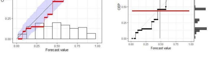
2
as the mean square error known as Brier’s score (1950). Although this statistic brought useful information,
it is only an average measure of the overall accuracy of such predictions. Analytical attributes of this
accuracy can be brought out such as Reliability, Resolution, Discrimination, Refinement to shed more light
on some qualities or deficiencies of issued forecasts. The purpose of this note is mostly pedagogical with
the aim to review the main tools available to that respect, and to illustrate them on data of a well-known
club competition with the UEFA champions League (also known in brief as C1) forecasted by simple
Poisson regression models. Focus is on a distribution-oriented approach based on the joint distribution of
elementary forecast, binary outcome pairs and its factorization. We will deal with several decompositions
of the Brier score (BRS) applied to each binary outcome considered separately namely 1) the Murphy
decomposition derived from the so-called Calibration-Refinement factorization (CR), and 2) the Likelihood-
base (LB) and Yates’s decompositions. In parallel to the CR decomposition, we will present a graphical
device known as the reliability diagram which allows diagnostic of strength or deficiency in this component.
In each case, comparison will be made between forecasts derived from a simple Poisson loglinear model
(POI), and to Bookmaker Odds implied probabilities (ODD). Finally, in the last (4th) section, we discuss the
main points raised by using these decompositions and possible implications for improving forecast
efficiency.
2 Decomposition of the Brier score
2.1 Basic theory
Let X be the binary outcome of the event H with probability q and P the random variable probabilistic
forecast of X taking values p. Taking as scoring rule, the quadratic or Half-Brier Score defined as the loss
2
function S ( P , X ) = ( P − X ) , and using the conditioning de conditioning rule, the Murphy (1973)
decomposition of its expectation can be written as
{
E [ S ( P , X )] = Var ( X ) − VarP E X ( X | P ) + E P E X ( X | P ) − P
2
}, (1)
where expectation is taken with respect to the pairs of forecasts and outcomes P , X .
Examination of this formula immediately identifies the 3 components of this decomposition:
1) Uncertainty (UNC) equal to Var ( X ) = q (1 − q ) , the variance of the outcome that is out of control
of the forecaster,
2) Resolution (RES) equal to VarP E X ( X | P ) referring to the variability between the conditional
expectations of the observed outcomes given their forecasts,
{ 2
}
3) Reliability (REL) or (Mis) Calibration equal to E P E X ( X | P ) − P measuring the average
squared differences between the conditional expectation of the outcome and its forecast.
Murphy and Winkler (1987) also gave the dual decomposition of (1)
{
E [ S ( P , X )] = Var ( P ) − Var X E P ( P | X ) + E X E P ( P | X ) − X
2
}. (2)
This decomposition is known as the Likelihood-base factorization as opposed to the Calibration-Refinement
factorization of formula (1) referring to the 2-way decomposition of the joint distribution of ( P, X ) . This
formula leads to identify three components: i) Refinement (REF) equal to Var ( P ) , the variance of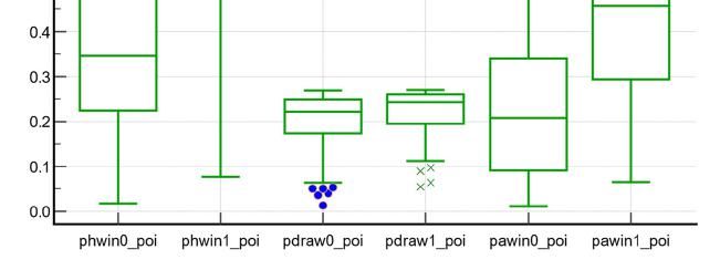
3
probabilistic forecasts also known as Sharpness, ii) Discrimination (DIS) equal to VarX E P ( P | X ) i.e.,
the variance between conditional distributions of forecasts given the outcomes X , iii) Conditional bias type
{ 2
}
2 as called by Bradley et al, (2003) equal to E X E P ( P | X ) − X which is the dual expression of
resolution. A special case of interest is the one with P having a probability mass function (pmf)
concentrated at p = E ( X ) , the mean of the marginal distribution of the binary outcome (the so-called
climatological forecast). Then the forecast has no refinement (Var P = 0) , no discrimination as well,
necessarily no resolution, even though it is perfectly calibrated. In fact, it is the only forecast being both
reliable with no discrimination (Bröcker, 2012). In that case, E[ S ( P, X )] reduces to its uncertain
component UNC as an upper reference value for the expected Brier score. That is the reason why the
decomposition in (1) is often expressed as fractions of UNC and the complement to one of the scaled Brier
Score (BS) as a Brier Skill Score
BSS = 1 − BS / BSref = ( REL - RES ) / UNC . (3)
This formula clearly emphasizes the trade-off between these two components with the aim of increasing
resolution without neglecting reliability.
There is another decomposition by Yates (1982) deserving as much attention as it defines influential
components of the expected quadratic score which are easier to understand:
E[ S ( P , X )] = Var ( X ) − 2 Cov ( P , X ) + VarX E P ( P | X )
2
(4)
+ E X VarP ( P | X ) + E ( P ) − E ( X ) .
2
This formula stems from the basic expression E[ S ( P , X )] = Var ( P − X ) + E ( P ) − E ( X ) with
Var( P ) = VarX E P ( P | X ) + E X VarP ( P | X ) and E ( P | X ) being the best predictor of P given
X . As this predictor is a linear one: E ( P | X ) = a + bX with a = E ( P | X = 0) ,
b = E ( P | X = 1) − E ( P | X = 0 ) , VarX E P ( P | X ) = b 2 Var ( X ) , Cov ( P , X ) = b Var ( X ) . These last
two expressions highlight the key role of the regression coefficient b of P on X equal to the difference
in expected value of forecasts pertaining to future positive outcomes from those out of negative ones.
Yates (1982) emphasized the different influence of the two components of Var( P ) . The first one, which
is the between class variance VarX E P ( P | X ) , he qualified as “VarPmin”, is beneficial. The second
one, which is the within class variance E X VarP ( P | X ) , called “∆VarP” or “Scattered Variance”
representing the lack of sharpness of the distributions of P | X = x , is detrimental. The last term in (4)
measures marginal bias and was called “Calibration or Reliability-in-Large” (CIL or RIL). In short, this
decomposition is written as: UNC- 2COV+ VarPmin+ ∆VarP+ RIL. Actually, Yates’ and the LB
decompositions are closely related although not subject to the same interpretation, with
REF=VarPmin+∆VarP, DIS= VarPmin and CB2=UNC-2COV+VarPmin+RIL.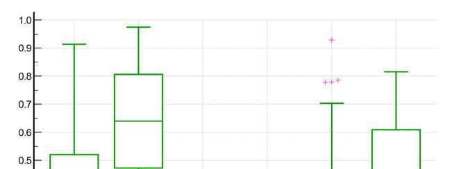
4
Table 1: Calibration-Refinement decomposition of Brier’s score pertaining to Home Win, Draw and Away
Win under the Poisson regression model.
RESULT BRS SKI (%) B-TEST UNC MET REL RES
INT 0.0035 (1.4) 0.0644 (26.2)
HWIN 0.1849 24.8 1.035 0.2458 QUA 0.0030 (1.2) 0.0639 (26.0)
[0.309] ISO 0.0116 (4.7) 0.0725 (29.5)
INT 0.0010 (0.5) 0.0036 (1.9)
DRAW 0.1849 1.4 3.995 0.1875 QUA 0.0031 (1.7) 0.0058 (3.1)
[0.045] ISO 0.0099 (5.3) 0.0125 (6.7)
INT 0.0047 (2.2) 0.0505 (23.4)
AWIN 0.1700 21.2 0.001 0.2158 QUA 0.0029 (1.3) 0.0487 (22.5)
[0.975] ISO 0.0078 (3.6) 0.0537 (24.9)
BRS=REL-RES+UNC with REL: Reliability, RES: Resolution, UNC: Uncertainty according to different binning
procedures (INT: Interval; QUA: Quantile: ISO-Regression).and expressed both in absolute value and p.100 of
uncertainty (UNC).
Skill (SKI) defined as SKI=(BRSref -BRS)/ BRSref where BRSref=UNC so that SKI=(RES-REL)/UNC
B-TEST: Brier-Score Test for departure of its expectation from that induced by the null hypothesis of perfect forecast
calibration expressed with its corresponding statistic and P-value within brackets.
2.2 Estimation from data
Practically, verification takes place from a data sample made of pairs {( pi , xi ), i = 1,..., N } of ex ante
probabilistic forecasts p i and ex post binary outcomes xi . Most quantities introduced previously can be
estimated by their regular moment estimators. The expected quadratic score E[ S ( P, X )] is traditionally
estimated by the empirical score:
S (p) = N −1 i =1 S ( pi , xi ) .
N
(5)
For the CR decomposition, REL and RES require estimations of E ( X | P ) . If the forecasts take K distinct
values { pk , k = 1,..., K } with nk occurrences of binary Noutcomes X , then
E k k k+ k k+ i =1 i
ˆ ( X | P = p ) = X = X / n with X = N I ( p = p )X and X =
k i
the Murphy (1973) decomposition is fully applicable without restrictions:
i =1 ( )
X i / N . In such cases,
REL = N −1 k =1 nk ( xk − pk ) , RES = N −1 k =1 nk ( xk − x ) , UNC = x (1 − x ) .
K 2 K 2
(6)
In fact, in many applications as in forecasting Football match results, we stay in-between discrete and
continuous distributions, facing many distinct forecast values. In such cases, forecasts have to be distributed
into intervals named bins B1 ,..Bd ,.., BD and averaged within bins i.e., letting I d = {i : pi ∈ Bd } , pairs
{ }
( pd , xd ), d = 1,..., D are computed as pd = nd−1 i∈I pi , xˆd = xd + / nd where nd = # I d ,
xˆd + = nd−1 i∈I xi . To avoid inconsistencies in the CR decomposition, two extra components of within
d
d
bin variance and covariance must be added to those in (6). We skip such complications by adopting a simple
N
procedure as advocated by Siegert (2017). Letting as in (5) S (xˆ ) = N
−1
S ( fi , xˆi ) and
N i =1
S ( x 1N ) = N −1
i =1
S ( fi , x ) with 1N , the unit vector of size N, the components of the mean score S (p)
reduce to
REL = S (p ) − S (xˆ ) , RES = S ( x 1N ) − S (xˆ ) , UNC = S ( x 1N ) . (7)5
This decomposition automatically satisfies the equality S (p) = REL − RES + UNC , and is equivalent to the
original Murphy decomposition in the case of distinct discrete forecasts. It also ensures that i) resolution is
nil when p is perfectly calibrated ( p = xˆ ), and ii) the constant climatological forecast p = x 1N is the only
forecast satisfying RES=REL=0. Finally, it is potentially applicable to other proper probabilistic scoring
rules, as the ignorance score L ( P, X ) = − X log( P) − (1 − X ) log(1 − P) (Dawid, 1986; Bröcker, 2012).
Moreover, the statistic 2 N L (p) − L ( qˆ p ) is an analog of the log-likelihood ratio statistic for a perfectly
reliable forecast having an asymptotic Chi-square distribution with degrees of freedom equal to the number
of parameters specifying the model for q p = Pr( X = 1| P = p ) .
Different binning techniques are available such as fixed threshold intervals and fixed quantile intervals with
potential optimization of their number (Bröcker, 2012; Gweon and Yu, 2019). A promising one relies on
the non-parametric isotonic regression implemented via the pool-adjacent-violators (PAV) algorithm with
optimality properties (Dimitriadis et al., 2021).
It also provides a reliability diagram featuring graphically the CR decomposition of the joint distribution
[ P, X ] = [ P ][ X | P ] of binned data by the marginal (refinement) distribution of forecasts and plots of (re)
calibrated probabilities xˆ d against automatically binned forecasts pd .
Table 2: Calibration analysis via fitting a logistic model of the probability of Homewin, Draw and
Awaywin (AWIN) on the logit of its probabilistic forecast under a Poisson regression model (POI)
Category Criterion Estimation SE T-Statistics DF P-value
intercept -0.259 0.119 4.700 1 0.030
Homewin slope 1.113 0.129 0.765 1 0.382
D0 vs D1 423.085 vs 417.489 5.596 2 0.061
intercept 0.153 0.466 0.108 1 0.742
Draw slope 0.932 0.346 0.039 1 0.843
D0 vs D1 426.981 vs 422.981 4.000 2 0.135
intercept 0.076 0.149 0.261 1 0.610
Awaywin slope 1.053 0.134 0.156 1 0.693
D0 vs D1 389.458 vs 389.176 0.282 2 0.870
Intercept (α) and slope (β) of the logit regression model with their estimation and standard error (SE).
Deviance D(k)=-2L(k) where L(k) is the loglikelihood of the null model (0: α=0; β=1) vs the unspecified
parameter model (1: α≠ 0; β≠ 0); T-statistics: Wald for intercept=0 and slope=1; Deviance differences
∆D=D0-D1 and their corresponding degrees of freedom (DF) and P-values
To that respect, another way to assess Reliability via the conditional distribution [ X | P ] of
outcomes X given P is through a regression model, but in the framework of logistic instead of linear
regression chosen by Reade et al. (2021). Following Cox (1958), the model relating X to P is
written via a logit linear predictor: logit Pr ( X i = 1) = α + β logit ( pi ) with α = 0 and β = 1 for
perfect reliability and typical patterns of reliability diagrams with i) (α > 0, β = 1) for concave
under-forecasting profiles, ii) (α < 0, β = 1) for convex over-forecasting profiles as well as iii)
(α = 0, β > 1) for sigmoid, and iv) (α = 0, β < 1) for inverse-sigmoid profiles. Statistical tests are
available (Wald and likelihood ratio tests) for challenging the different hypotheses about such
patterns.6
3 Application
The purpose of this illustration is to assess the performance of probability forecasts of outcomes of the
UEFA champions league (the so called C1) matches played during the group stage (GS). Four seasons were
considered from 2017 to 2020. Forecast is based on a simple log linear Poisson regression model applied to
score lines with intercept, home effect and two time-dependent ELO team covariates. The models was fitted
to ex ante data, namely score lines of all the matches played during the 3 previous seasons e.g., 2017, 2018
and 2019 as training sample to forecasts of the 96 GS matches of 2020; the same applies to forecasts of the
2019 GS based on 2016, 2017 and 2018 seasons and so on. Inference about parameters of the Poisson
loglinear model is based on posterior distributions and probability forecasts are obtained as expectations of
predictive distributions. Computations are carried out via the Win/OpenBUGS software. As top reference,
we considered the classical Bookmaker Odds (ODD) as 3-Way Odds implied Probabilities with probabilities
3
derived as p m , j = om−1, j / o −1 where o m , j is the betting odd for j = 1, 2, 3 (WDL) edited by
k =1 m , k
OddsPortal (here an average of 10 to 12 odds from well-known betting companies).
Table 3: Characteristics of conditional distributions of probability forecasts given the outcomes under two
Forecasting procedures: Poisson regression (POI) and Odds Probabilities (ODD)
Method Home Win Draw Away Win
POI ODD POI ODD POI ODD
Sample sizes 217-167 288-96 263-121
X=0 37.88 35.01 20.22 20.97 24.30 23.24
Mean % X=1 63.08 62.73 22.34 23.89 44.84 48.62
Dif 1-0 24.20 27.71 2.02 2.93 20.54 25.38
Wilcoxon Z 9.93 10.76 3.59 3.55 9.09 10.13
P-val7
d =1 i=1 I ( pi ∈ bd , bd +1 ) ( qd − pi )
D N 2
, (8)
under the constraints of isotonicity ( qd estimation is a non-decreasing function of the original pi ’s). Results
are displayed in Table 1, for Home Win, Draw and Away Win categories considered separately in terms of
absolute values of Mean Brier score and its components (REL, RES, ACC) and Skill. Lack of reliability
turns out to be small (lower than 5.5% of UNC) with miscalibration estimated a little bit higher under iso-
regression. These values are supported by statistics and P values of Brier’s score tests of departure from
zero miscalibration (Spiegelhalter, 1986; Sellier-Moiseiwitch and David, 1993).
Figure 1: Reliability Diagrams for Home Win Probability Forecasts with plots of the Conditional
Probability Events (CEP) against the Forecast Probability Values via Iso Regression. On the left :
Reliability with Point 95% Consistency Bands. On the right: Discrimation diagrams with marginal
distributions of forecasts and calibrated values.
Skill values are also appreciable for Home win (25 to 30%) and Away win (20 to 30%) with a little
advantage of Odds vs Poisson of around 5. On the opposite, skill remains quite poor for Draw: 1.4 to 3.0%
for Poisson and Odds respectively. Corresponding reliability diagrams were produced with an example
shown for Home Win under Poisson and forecasts on Fig 1. There is some evidence of over-forecasting for
Home Win practically all over the forecast range for Poisson, and at least, below p8
outcomes. Characteristics of these two distributions are given in Table 3 and Fig 2. Differences between the
means of these two conditional distributions are much more marked for Home Win and Away Win than for
Draw. Again, these differences are more pronounced with Odds than Poisson as also reported by the Harrell
c-statistics around 0.8 for Home Win and Away Win, and only 0.6 for Draw. Graphically, the boxplots
confirmed this situation showing a clear separation of the two distributions for Home Win and Away Win
and a tiny one for Draw.
Detailed accounts of Yates’ and LB decompositions are shown on Table 4. In short, what emerges from
them lies in the large role and weight given to the covariance component: 41 to 48% for Home Win and
Away Win under Poisson and 50 to 55% with Odds with nevertheless a non-negligible part devoted to
“noise” variance of forecasts (15 to 18%). The same picture applies to Draw but with much more tiny
components, especially discrimination and covariance.
Table 4: Yates’s and LB decompositions of Brier’s score pertaining to Home Win, Draw and Away Win
under the Poisson regression model (POI)
Factors Home Win Draw Away Win All
value % value % value % value %
UNC 0.2458 100.0 0.1875 100.0 0.2158 100.0 0.6490 100.0
(-2)COV -0.1190 -48.4 -0.0076 -4.0 -0.0886 -41.1 -0.2150 -29.5
VPB 0.0144 5.8 0.0001 0.0 0.0091 4.2 0.0236 3.6
VPW 0.0413 16.8 0.0031 1.7 0.0336 15.6 0.0780 12.0
RIL 0.0024 1.0 0.0017 0.9 0.0000 0.0 0.0042 0.6
REF 0.0556 22.6 0.0032 1.7 0.0427 19.8 0.1016 15.6
-DIS -0.0144 -5.8 -0.0001 -0.0 -0.0091 -4.2 -0.0236 -3.6
CB2 0.1436 58.4 0.1817 96.9 0.1363 63.2 0.5396 83.
BRS 0.1849 75.2 0.1848 98.6 0.1700 78.8 0.5397 83.1
Yates’s decomposition into 5 components as follows BRS=UNC-2COV+VPB+VPW+RIL with UNC:
Uncertainty, COV: Covariance between forecast and outcome, VPB: Variance among means of probability
forecasts with outcome=1 and outcome=0, VPW : Average of Within groups variance and RIL marginal
bias squared between the two groups, according to forecasting procedures (POI and ODD models) .
Likelihood base decomposition into 3 components BRS=REF-DIS+CB2 with REF: Refinement or
Sharpness of forecast variance, DIS=Discrimination same as VPB and CB2: Type 2 bias equal to VPW-
2COV+RIL.
4 Discussion
This presentation was deliberately restricted to the most popular (strictly) proper scoring rules as this
properness property is a cornerstone of decision theory based on minimizing expected loss (or maximizing
utility) (Bernardo, 1979; Gneiting and Raftery, 2007). They provide an incentive for ex ante honesty and
reward ex post accuracy. Little was said about verifying probability forecasts for multiple categories taken
simultaneously. Probability scoring rules are extended easily to that situation as shown in Table 4 for Yates’
decomposition. Unhappily, such an extension is not straightforward for the CR decomposition. One reason
for that lies on how to define bins. Procedures have been proposed to that respect by Broecker (2012) based
on some functions of the probability vector for the J multiple categories of interest. A simple way to handle9
the multiclass setting is by treating the problem as J one-versus-all binary events via e.g., a logistic-type
regression with standard normalization of outcome probabilities. More generally, such forecasting
verification methods already gained much attention in other fields especially in machine learning especially
due to miscalibration of neural networks and its applications to health and medicine (Guo et al, 2017).
Figure 2: Box-plots of the conditional distributions of probabilistic forecasts of binary events (Home Win,
Draw and Away Win) given the observed outcomes (X=0) and (X=1) and according to the Poisson
loglinear regression (poi)
Although much of the theory and applications originated from meteorological literature (Winkler and
Murphy, 1979; Jolliffe and Stephenson, 2003; Wilks, 2011), there had been a few attempts to apply some
of these analytical procedures to football match results, especially in the EPL (Forrest and Simmons, 2000;
Selliti Rangel, 2018; Wheatcroft, 2019; Read et al, 2021) but not enough. This area would benefit from a
more systematic utilization. Regarding our application to the UEFA Champions League, it turns out that
forecasts of Away Wins is both well calibrated and refined with good discrimination properties. The same
trend can be seen on Home Wins, but with a trade-off between that over-forecasted category and under-
forecasted draws with little discrimination of draw forecasts. It looks as if this category stands apart from
the two others.
References
Bradley, A. A., T. Hashino, and S. S. Schwartz. (2003), ”Distributions oriented verification of probability
forecasts for small data samples”, Weather Forecasting ,18, 903–917.
Brier, G. (1950), “Verification of forecasts expressed in terms of probability”, Monthly Weather Review,
78, 1-3.10 Bröcker, J. (2012) Probability forecasts. In Forecast Verification: A Practitionner's Guide in Atmospheric Science, Second Edition. Edited by l. T. Jolliffe, and D.B. Stephenson. 2012 John Wiley & Sons, pp 119- 139. Cox, D.R. (1958), “Two Further Applications of a Model for Binary Regression”, Biometrika, 45, 562-565. Dawid, A. P. (1986), “Probability Forecasting”, Encyclopedia of Statistical Science, 7, 210-218. Dimitriadis, T. Gneiting, T. and Jordan, A.I. (2021) Stable reliability diagrams for probabilistic classifiers. Proceedings of the National Academy of Sciences of the United States of America 118 (8) DOI: 10.1073/pnas.2016191118 Forrest, D., and R. Simmons. (2000), “Forecasting Sport: The Behaviour and Performance of Football Tipsters”, International Journal of Forecasting, 16, 317-331. Gneiting, T., and A.E. Raftery. (2007), “Strictly Proper Scoring Rules, Prediction, and Estimation”, Journal of the American Statistical Association, 102, 359–378. Guo, C., Pleiss, G., and K.Q., Weinberger.(2017), ”On Calibration of Modern Neural Networks”, arXiv: 1706.04599v2 Gweon, H., and H. Yu. (2019), “How reliable is your reliability diagram? “ Pattern Recognition Letters, 125, 687-693. Jolliffe, I., and D. Stephenson. (2003), “Forecast Verification: A Practitioner’s Guide in Atmospheric Science”, John Wiley-Blackwell Murphy, A.H. (1973), “A new vector partition of the probability score”, Journal of Applied Meteorology, 12, 595–600. Murphy, A. H., and R.L., Winkler. (1987), “A general framework for forecast verification”. Monthly Weather Review ,155, 1330-1338. Reade, J. J., Singleton C., and A. Brown. A. (2020) Evaluating Strange Forecasts: The Curious Case of Football Match Scorelines. Scottish Journal of Political Economy, 68, 261-285. Scarf, P., and J. Selliti Rangel Jr. (2016), “Models for outcomes of soccer matches”. In Handbook of Statistical Methods and Analyses in Sports, Eds by J. Albert, M.E., Glickman, T. B, Swartz ,and R.H. Koning, 341-354. CRC Press, Chapman pp. 341-354. Seillier-Moiseiwitsch, F., and Dawid, A.P. (1993), “On Testing the Validity of Sequential Probability Forecasts”, Journal of the American Statistical Association, 88, 55-359. Selliti Rangel Jr, J. (2018), “Estimation and Forecasting Team Strength Dynamics in Football: Investigation into Structural Breaks”, PhD thesis, University of Sallford, UK. Siegert, S. (2017), “Simplifying and generalising Murphy’s Brier score decomposition.” Quarterly Journal of the Royal Meteorological Society, 143, 1178–1183. Spiegelhalter, D. J. (1986), “Probabilistic prediction in patient management and clinical trials”, Statistics in Medicine 5, 421–433. Wheatcroft, E. (2019), ”Interpreting the skill score form of forecast performance metrics”, International Journal of Forecasting, 35, 573-579. Wilks, D. S. (2011), “Statistical Methods in the Atmospheric Sciences”, 3rd Edition Academic Press, Oxford. Winkler, R.L., and A.H. Murphy. (1979), “The Use of Probabilities in Forecasts of Maximum and Minimum Temperatures”, The Meteorological Magazine, 108, 317-329. Yates, J.F. (1982), “External correspondence: Decompositions of the mean probability score”, Organizational Behavior and Human Performance, 30, 132–156.
You can also read