Methodology for Modelling Distributional Impacts of Emissions Budgets on Employment in New Zealand - Lynn Riggs Livvy Mitchell July 2021

Motu Working Paper 21-14

Methodology for Modelling
Distributional Impacts of
Emissions Budgets on
Employment in New Zealand

Lynn Riggs
Livvy Mitchell
July 2021

Methodology for Modelling Distributional Impacts of Emissions Budgets on Employment in New Zealand

Document information
Author contact details
Lynn Riggs
Motu Economic and Public Policy Research
PO Box 24390
Wellington 6142
New Zealand
Email: lynn.riggs@motu.org.nz

Acknowledgements
This research was supported by the Climate Change Commission. The employment results modelled in this
project are simulated based on employment data provided by Statistics New Zealand and based on
employment projections provided by Niven Winchester and Dominic White. We thank Niven Winchester,
Dominic White, Karen Lavin, Anita King, and Carly Soo for insightful comments on earlier drafts. We also thank
Corey Allan for his support of this project, and we thank Dave Maré and Richard Fabling for their work in
developing and maintaining the labour tables upon which this research is based.

Disclaimer
Access to the data used in this study was provided by Stats NZ under conditions designed to give effect to the
security and confidentiality provisions of the Statistics Act 1975. The results presented in this study are the
work of the authors, not Stats NZ or individual data suppliers.

These results are not official statistics. They have been created for research purposes from the Integrated Data
Infrastructure (IDI) and Longitudinal Business Database (LBD) which are carefully managed by Stats NZ. For
more information about the IDI and LBD please visit https://www.stats.govt.nz/integrated-data/.

The results are based in part on tax data supplied by Inland Revenue to Stats NZ under the Tax Administration
Act 1994 for statistical purposes. Any discussion of data limitations or weaknesses is in the context of using the
IDI for statistical purposes and is not related to the data’s ability to support Inland Revenue’s core operational
requirements.

Motu Economic and Public Policy Research
PO Box 24390 info@motu.org.nz +64 4 9394250
Wellington www.motu.org.nz
New Zealand

© 2021 Motu Economic and Public Policy Research Trust and the authors. Short extracts, not exceeding two
paragraphs, may be quoted provided clear attribution is given. Motu Working Papers are research materials
circulated by their authors for purposes of information and discussion. They have not necessarily undergone
formal peer review or editorial treatment. ISSN 1176-2667 (Print), ISSN 1177-9047 (Online).

 i

Methodology for Modelling Distributional Impacts of Emissions Budgets on Employment in New Zealand

Abstract
Efforts to reduce emissions to counter climate change are expected to have both costs and
benefits, and these effects are likely to be unevenly distributed across the population. Hence, we
developed the Distributional Impacts Microsimulation for Employment (DIM-E) to examine the
potential distributional employment impacts for different mitigation options to reduce
greenhouse gas emissions. DIM-E is comprised of two main components: the first component
estimates industry-level employment effects, and the second simulates the characteristics of
impacted workers and jobs. We based DIM-E on results from a computable general equilibrium
(CGE) model, C-PLAN, and applied them to more detailed employment information in order to
better understand the extent to which industries, jobs and workers are likely to be impacted by
the different pathways. It is possible, however, for DIM-E to be used to analyse any policy
scenario and its baseline using employment indices and similar employment information. In this
paper, we describe DIM-E in the context of the initial case for which it was developed – to
analyse emissions budgets for greenhouse gasses to be set by the New Zealand government for
three time periods (2022-2025, 2026-2030, and 2031-2035). We also provide a sampling of
results from this initial case in order to put the methodology into context. Hence, we show that
DIM-E can be used to examine changes in employment trends due to policy changes as well as
the different types of workers that are most likely to be affected by the reallocation of
employment across industries. We found that the DIM-E results produced for the initial case
were in line with previous research in this area – the overall net industry employment effects
were predicted to be relatively small, though some industries will be more affected than others
especially in the short- and medium-term. Moreover, very few worker groups would be
negatively affected (in terms of the number of jobs) by any of the proposed mitigation options
especially over the long term.

JEL codes
J01, Q52, R11

Keywords
Environmental Economics, Climate Change Mitigation, Distributional Impacts of Employment

 ii

Methodology for Modelling Distributional Impacts of Emissions Budgets on Employment in New Zealand

Table of Contents
1. Introduction 1

2. The Pathways and Current Policy Reference 4

3. Methodology 5
 1.1 Data 5

 1.2 Downscaling CGE Model Results 7

 1.3 Simulation of Worker-Job Characteristics 15

4. Sample of Results from DIM-E Worker-Job Simulation 16

5. Discussion 18

6. Conclusion 21

7. Tables 25

8. Figures 28

9. Appendix 38

Table of Figures
Figure 1. Employment Indices from C-PLAN for Agriculture before (top panel) and after (bottom panel)
Productivity Adjustment for Draft Advice, 2014-2050 28

Figure 2. Cumulative Employment Changes (WJE) in Sheep, Beef Cattle and Grain Farming (A014) 29

Figure 3. Average Annual Employment Changes (WJE) Predicted in each Time Period 30

Figure 4. Industry Distribution of Cumulative Net Employment Effects (Gains, Losses, and Total Net) under TP4
from Publicly Available Employment Data 31

Figure 5. Industry Distribution of Cumulative Total Net Employment Effects under TP4 from Publicly Available
Employment Data 32

Figure 6. Counts of Simulated Worker-Jobs by Net Effect Type for 2022-2025 (Left Panel) and for 2022-2050
(Right Panel) 33

Figure 7. Simulated Worker-Job Annual Earnings by Net Effect Type for 2022-2025 (Left Panel) and 2022-2050
(Right Panel) 34

Figure 8. Cumulative Net Effects by 1-digit Industry for Draft Advice, 2022-2050 35

Figure 9. Share of Net Worker-Jobs by Highest Qualification for 2022-2025 36

Figure 10. Detailed Shares of Net Effects by Highest Qualification for 2022-2050 37

 iii

Methodology for Modelling Distributional Impacts of Emissions Budgets on Employment in New Zealand

1. Introduction
Efforts to reduce emissions to counter climate change are expected to have both costs and
benefits, and these effects are likely to be unevenly distributed across the population. Hence, we
developed the Distributional Impacts Microsimulation for Employment (DIM-E) to examine the
potential distributional employment impacts for different mitigation options to reduce
emissions1. DIM-E is comprised of two main components: the first estimates industry-level
employment effects, and the second simulates the characteristics of impacted workers and jobs.
We based DIM-E on results from a computable general equilibrium (CGE) model, C-PLAN2.
However, employment indices from any policy scenario and its baseline could be used.
 In this paper, we describe DIM-E in the context of the initial case for which it was
developed – to analyse emissions budgets for greenhouse gasses to be set by the New Zealand
government for three time periods (2022-2025, 2026-2030, and 2031-2035). Since there are
many different policy-mix options that could be used to meet these budgets, the New Zealand
Climate Change Commission developed different pathways which were simulated over these
time periods to ensure that their proposed budgets were achievable. These pathways were
modelled using C-PLAN to assess the potential economic effects of these different options. We
used projected employment indices from C-PLAN under these different pathways and applied
them to more detailed employment information in order to better understand the extent to
which industries, jobs and workers are likely to be impacted by the different pathways.
 Most of the systematic, quantitative research in the international literature relating to
within-country distributional impacts of climate change policies primarily assesses the impact of
carbon pricing on household energy bills, household incomes, or overall employment levels.
(Büchs et al., 2011; Gough, 2013; Goulder et al., 2019; Longhi, 2015; Nikodinoska & Schröder,
2016; Preston et al., 2010; Rausch et al., 2011; Schaffrin & Reibling, 2015; Wang et al., 2016;
White & Thumim, 2009). There is little quantitative research on the effects of these policies, or
even the effects of climate change itself, on employment in terms of the types of jobs and
workers most likely to be affected. Hsiang et al. (2017) estimate economic damage at the US
county level from climate change using low- and high-risk labour3 as one of many outcome

1 The initial case was to examine the effects of mitigation efforts to achieve net zero emissions of long-lived gases and to
reduce biogenic methane emissions by 24-47% by 2050 in New Zealand.
2 The C-PLAN model is a global, recursive, dynamic CGE model tailored to the economic and emissions characteristics of

New Zealand. (Winchester & White, 2021)
3 This article categorises jobs into two groups: low-risk and high-risk. Low-risk jobs are defined as those where workers are

minimally exposed to outdoor temperatures, and high-risk jobs are defined as those who are heavily exposed (construction,
mining, agriculture, and manufacturing).
 1

Methodology for Modelling Distributional Impacts of Emissions Budgets on Employment in New Zealand

measures (e.g., agricultural yields, mortality, crime); however, this paper provides little detail
about those groups most likely to be affected.
 Relatively few papers have examined the distributional effects of environmental policies
on employment. Roland-Holst et al. (2020) is one example of a study that downscaled results
from a CGE model to examine net job creation (using Full-Time Equivalent (FTE) jobs) by county
in an assessment of the US state of Oregon’s Cap-and-Trade Program.4 They found most counties
in the state experienced small FTE changes (between 0 and 1000) by 2050; however, the report
did not include an analysis of job changes by industry, job, or worker characteristics.
 Hafstead & Williams (2020) provide a general review of the literature and a thorough
discussion about the policy questions related to employment in this area. In this article, the
authors concluded that existing research provides clear answers to some questions. For
example, existing research indicates that changes in jobs due to policies are primarily
reallocations across industries as opposed to substantial aggregate effects such as large net job
gains or net job losses. Moreover, most of this reallocation occurs via less hiring rather than
through separations.5 They find that both results hold even for large, economy-wide policies.
The latter result, however, may depend on the policy design (scale, scope, and implementation
speed), but even so, policy design has a greater impact on short-term outcomes6 and has little
effect on the long term. Pre-announcements (as found in Hafstead & Williams (2019)) and
phasing-in policies have also been found as measures to counter some of the short-term effects
caused by these policies. In summary, research in this area has generally shown that
environmental policy has little effect on overall employment – particularly in the long run.
 Hafstead & Williams (2019) is one of the few papers that focused on employment effects
for workers in different industries. They used an extension of the search-CGE model (based on
US labour markets) from Hafstead et al. (2018) which included industry switching frictions and
staggered wage bargaining using three different types of environmental policies. In this model,
the authors followed simulated workers based on their industry when the policy was
implemented. These industries were categorised as follows: mining industries, utility industries,
manufacturing industries, and other industries. Hafstead & Williams (2019) concluded that the
short-run differences (less than 18 months) in unemployment rates (including size and duration)
between the policies and the business-as-usual scenario largely depended on two things: the

4 This analysis assumed that future jobs would be created in the locations where the current jobs exist because there was
not enough information available to predict the locations of these new jobs.
5 However, the authors note that this may be less true for already declining industries – these industries may have already

reduced hiring substantially and hence increased job separations may be the only viable option remaining.
6 This is particularly true for distributional effects the policy design is such that layoffs are required given that layoffs tend to

increase the duration of unemployment and are more likely to lead to persistent negative effects for these workers.
 2

Methodology for Modelling Distributional Impacts of Emissions Budgets on Employment in New Zealand

ease with which workers could change industries and the magnitude of reallocation across
industries caused by the policy.7 This was particularly true for workers in mining and utilities 8.
Moreover, in their model, some high-turnover sectors like coal mining, which had high
unemployment rates even without the policy, had lower unemployment rates in the medium
term under the policy as it accelerated workers movement into lower-turnover sectors. The
switching friction was also found to be relatively unimportant in determining the unemployment
rate across all workers.
 In this paper, we describe the DIM-E methodology and provide a sampling of results in
order to put the methodology into context9. DIM-E can be used to examine changes in
employment trends due to policy changes as well as the different types of workers that are most
likely to be affected by the reallocation of employment across industries, which is one area
highlighted in Hafstead & Williams (2020) as needing more research. In so doing, we hope that
DIM-E can be used to target policy to help reduce search frictions and improve worker mobility
which should ultimately reduce the short-term negative effects of the reallocation.
 In line with previous research in this area, our initial analysis using DIM-E indicates that the
overall net employment effects estimated in this analysis are predicted to be relatively small,
though some industries will be more affected than others especially in the short- and medium-
term. In fact, the industry rankings of the top net negative and top net positive industries using
cumulative changes were fairly consistent across the four time periods and across the four
pathways that we analysed.10 On the net positive side, transport Industries tended to dominate
the industry rankings, and in later periods, some agricultural industries also tended to rank
highly (e.g., Dairy Cattle Farming and Sheep/Beef Farming). On the net negative side, various
manufacturing industries tended to dominate the top ranks; however, the Oil and Gas Extraction
industry was also consistently in the top ranks.
 Our DIM-E results also indicated that very few groups would be negatively affected (in
terms of the number of worker-jobs) by any of the proposed pathways especially over the long
term. Workers holding jobs in Mining, Manufacturing, and Electricity, Gas, Water and Waste

7 More reallocation was better for workers as it provided more opportunities to move.
8 Castellanos & Heutel (2019) found similar results using a static model to compare results when assuming perfect mobility
between jobs to those assuming perfect immobility. They found little overall effect on the aggregate unemployment rate
but more substantial differences for unemployment of workers in the oil and gas extraction sector and in the coal mining
sector (more negativity affected under perfect immobility). They also found that policy design could be used to mitigate
these effects.
9 For demonstration purposes, we will use publicly available data to generate some results included in the paper as

representative of the types of analyses that can be done using DIM-E. Primarily, these will be results that would have more
difficulty passing the confidentiality protections of Statistics New Zealand.
10 The net effects are in terms of the pathway results compared to the current policy scenario. Hence, industries that are

net positive have more employment under the pathway than under the current policy scenario, and net negative industries
have less employment under the pathway than under the current policy scenario.
 3

Methodology for Modelling Distributional Impacts of Emissions Budgets on Employment in New Zealand

Services will be negatively affected, but Manufacturing more so than the other two industries.
Workers holding jobs in Taranaki and the West Coast are also expected to be negatively affected
under all four pathways by the end of the period; however, this is largely due to the
concentration of negatively affected industries located in these regions. Given that the negative
employment effects will likely outweigh the positive employment effects in these regions, these
workers may have more difficulty transitioning into new sectors.
 It is important to remember that DIM-E is a model and that the simulated results derived
from the model need to be taken in context. Models such as DIM-E and C-PLAN are generally
designed to better understand the implications of different actions and assumptions and to
provide insights into the effects that could potentially occur under certain scenarios – they are
not designed to exactly predict the future. Hence, any of the DIM-E results must be interpreted
carefully, drawing on the scenario details and the outputs from the model used to generate the
employment indices (in this case C-PLAN).
 The remainder of the paper is organised as follows. Section 2 describes the transition
pathways that were used as the basis for the initial analysis. Section 3 describes the DIM-E
methodology, including information about the data, the CGE model, and the simulation model.
Section 4 presents results to demonstrate DIM-E’s functionality, Section 5 provides further
discussion, and Section 6 concludes.

2. The Pathways and Current Policy Reference
There are a number of different ways that New Zealand could use to reduce greenhouse gas
emissions to its targeted levels by 2050, and different mitigation options to achieve these results
were considered. The Climate Change Commission (CCC) considered four different scenarios to
achieve the proposed emissions budgets, called transition pathways, in developing its draft
advice.
 All pathways considered two baskets of emission prices that factor in the split gas target11,
one for biogenic methane and one for all other gases. Transition Pathway 1 (TP1) was designed
to set out the central assumptions across the energy and land system while the other three
transition pathways were designed to test different mitigation options and technology
uncertainties by deviating from these central assumptions in different ways. For example,
Transition Pathway 2 (TP2) focused on methane technology and combined quicker uptake of
methane reduction technologies with tighter methane targets. Transition Pathway 3 (TP3)

11The split gas target is to achieve net zero emissions of long-lived gases and to reduce biogenic methane emissions by 24-
47% by 2050.
 4

Methodology for Modelling Distributional Impacts of Emissions Budgets on Employment in New Zealand

constrained forestry removals in order to identify the costs of relying more heavily on emissions
reductions. Transition Pathway 4 (TP4) focused on faster reductions and was designed to test
the impacts of adopting more ambitious near-term emissions reduction targets for non-biogenic
methane. As a baseline, a scenario was also developed to simulate the New Zealand economy
under “business as usual” assumptions. This is called the Current Policy Reference scenario
(CPR). The main differences between the CPR and the transition pathways are shown in Table 1.
 For the CCC’s final advice, they considered a fifth transition pathway using an updated
CPR. The updated CPR aligns more closely with baseline assumptions used in other modelling
commissioned by the CCC including but not limited to assumptions on removals, land use,
agricultural productivity, agricultural and waste emissions intensity, electricity generation,
electric vehicle uptake, and oil prices. The fifth transition pathway used for the final advice was
designed to reduce emissions faster than the original four pathways to achieve net zero by 2040
rather than by 2050.

3. Methodology

1.1 Data
We used data sourced from Statistics New Zealand’s Integrated Data Infrastructure (IDI) and
Longitudinal Business Database (LBD).12 These data include population-wide, linked
administrative, census, and survey data for people and businesses. Each individual person or
entity is given a unique identification number which allows them to be linked across different
data sets. This allowed us to observe establishment- and enterprise-level information related to
the business or businesses for which an individual works as well as information about individuals
themselves.
 Within the LBD, data are provided at different levels of the business including the
enterprise level and the geographic unit level. The enterprise level pertains to a tax-reporting
legal entity (e.g., sole proprietor, partnership, company). In the data, each enterprise is given a
unique, permanent enterprise number (“PENT”) to allow the enterprise to be tracked over time,
even if there is a change in the type of legal entity.13 Geographic units are establishments of the
enterprise (e.g., a grocery store chain would be represented in the data as the enterprise and
each store would be considered a geographic unit). These establishments could be storefronts,

12 For more information about these data, see the Statistics New Zealand website.
13 For example, if a partnership decides to change to a limited liability company but is otherwise essentially the same entity,
its PENT should remain the same.
 5

Methodology for Modelling Distributional Impacts of Emissions Budgets on Employment in New Zealand

headquarters, warehouses, or plants. Each establishment has been given a permanent unique
identifier (“PBN”), which allowed us to track continuing activity at the same location.
 Our analysis primarily relied on the monthly, linked employee-employer data to connect
individual-level worker data in the IDI with business-level data in the LBD. 14 This allowed us to
observe both establishment- and enterprise-level information for each employee as well as
information about the workers themselves (e.g., age, gender, ethnicity). The unit of observation
in the monthly data set is a worker-job, which we defined as the employment relationship
between a worker and a single enterprise.15 Each worker-job is assigned to an establishment,
and the industry and region for each worker-job is based on the establishment’s industry and
region.16 For these analyses, we used the group level of the ANZSIC06 codes to define
industries.17 We use the group level since it provides sufficiently distinct production activities
while still providing sufficient aggregation of workers and businesses across most categories to
protect confidentiality.
 We used these data for the 2014 calendar year – the base year for the employment indices
from C-PLAN – to estimate the number of worker-jobs in each ANZSIC06 industry code.18 This
was done by counting the number of unique worker-jobs in each month and averaging over the
course of the year.
 We also used worker-jobs data for the 2018 calendar year19 to describe characteristics of
the workers in these jobs using unique worker-jobs over the course of the year. In addition to
estimating characteristics for all worker-jobs, we estimated the characteristics for two mutually-
exclusive sub-samples – worker-jobs with at least one short spell of work during the year (“short-

14 More detailed information about the LBD can be found on the Statistics NZ website and in Fabling and Sanderson (2016).
15 Individuals appear in these data more than once if they have multiple jobs with different enterprises. However, if a
worker was reassigned to a different location within the same enterprise, this is not counted as a new worker-job because
the enterprise remains the same and only the enterprise changes.
16 Note also that establishments and enterprises can be assigned separate industry codes, and these can even differ across

the broadest industry classification level – the 1-digit ANZSIC06 industry classifications, called the division level, is the
broadest level.
17 More information about the ANZSIC2006 system can be found in Trewin & Pink (2006).
18 We cleaned the data such that a worker-job can only be assigned to one ANZSIC06 industry code. It is possible for

establishments to switch industry codes during a year, so to avoid double-counting worker-jobs in this instance, we
replaced a worker-job’s industry code to equal the most frequent ANZSIC06 code over the months for which the worker-job
is observed during the year. When multiple industry codes were observed for the same number of months, we selected the
lowest industry code (e.g., if the worker-job is observed in A011 for 6 months and in A012 for 6 months, the worker-job will
be assigned to A011). However, these instances were infrequent. Workers could also be assigned to multiple
establishments within the enterprise over the course of a year, and we used a similar methodology to assign workers to a
single establishment within the enterprise during the year.
19 We used 2018 for two reasons. Firstly, it was the most complete year of data available when we began the analysis.

Secondly, it allowed us to link with 2018 Census data in order to obtain more detailed information about workers.
 6

Methodology for Modelling Distributional Impacts of Emissions Budgets on Employment in New Zealand

spell worker-job”) and worker-jobs with no short spells during the year (“not-short-spell worker-
job”).20
 For demonstration purposes, we will also use publicly available data 21 from Statistics New
Zealand to simulate some results that might otherwise be problematic to have released. These
data are from the official quarterly statistics produced from the Linked Employer-Employee Data
(LEED) made available by Statistics New via NZ.Stat. Since these data are quarterly, we use the
annual average for the year. For example, we use data on filled jobs in 2014 from the LEED
measures by industry (based on ANZSIC06) to show the industry-level distribution of affected
jobs.
 This component of the analysis used data from a variety of sources. For example, we
merged 2018 Census data with the worker-jobs data to obtain workers’ highest educational
attainment. We used data for all worker-job months in 2018 and aggregated these to the annual
level for each ANZSIC06 code listed in the Appendix.
 Across multiple datasets in the IDI, we observed the following characteristics of workers:
gender, ethnicity, age, highest qualification, migrant status22, and number of jobs held per
month. For worker-job characteristics, we used earnings from wages and salaries23, Full-Time
Equivalent (FTE)24, and region. We also distinguished worker-jobs that had at least one starting
month during the year (“starts”), at least one ending month during the year (“ends”), and no
start or end months during the year (“continuers”). These data provided the basis for the annual
counts and averages per worker-job in each industry.

1.2 Downscaling CGE Model Results
We used the employment indices generated by C-PLAN25 which used 2014 as the base year and
included projections through 2050.26 For these calculations, C-PLAN assumed full employment
using a natural unemployment rate of 4.5% in the modelling for the CCC’s draft advice, which
was based on the long-term unemployment rate used in the Treasury’s Long-Term Fiscal Model.

20 A short spell is defined as a period of employment without an interior month, and thus consists only of a start and end
month. Hence, short spells, by definition, are less than 3 months in duration. See Fabling and Maré (2015) for more details
about the derivation of the data.
21 These data are more aggregated than the data that is available in the data labs. Hence, these data are just used to

demonstrate the types of analyses that can be conducted using LEED, but the results using these data are not necessarily
the same as those found using the confidential data sets.
22 This was a binary variable depending on whether the worker had a visa accepted in the MBIE immigration data.
23 These are administrative data submitted to Inland Revenue by employers who deduct and pay PAYE (pay as you earn)

income tax on employees’ behalf.
24 This measure is based on worker’s earnings in the month relative to the minimum wage as described in Fabling and Maré

(2015).
25 More details about C-PLAN are provided in Winchester & White (2021)
26 From the CGE model, the relevant parameter for employment is Employment (f,i,r,t) where f represents production

factors, i represents industries, r represents regions (New Zealand or the rest of the world), and t represents time (annual).
This parameter reports an employment index (EI) for each sector equal to one in the base year (2014) for each sector.
 7

Methodology for Modelling Distributional Impacts of Emissions Budgets on Employment in New Zealand

(Piscetik & Bell, 2016) For the final advice, the unemployment rate used in the modelling was
4.25% to align with the Treasury’s Fiscal Strategy Model Projections.
 The full-employment assumption requires employment losses to be offset by employment
gains in other sectors of the economy, and hence, employment growth is based on expected
population changes. One critique of using full-employment CGE models for estimating
employment effects is that these models do not account for frictional, structural, or cyclical
unemployment. (Hafstead et al., 2018) However, CGE models like C-PLAN are generally meant to
be used for mid- and long-term projections (a decade or longer) – they are not designed to look
at short-term outcomes (e.g., annual or shorter) because most of these models do not fully
account for short-term fluctuations due to economic shocks or the business cycle. (Chen et al.,
2016) While the full-employment assumption may be unrealistic to examine employment
changes in the short run, over longer time periods, economies generally fluctuate around full
employment.
 To better understand the potential effects of the full employment assumption, Hafstead et
al. (2018) compared a full-employment CGE model (which assumed that labour markets fully
clear) to a search-CGE model (which introduced a search friction) in order to compare changes in
aggregate and industry-level employment from different environmental policies.27 Their results
showed that both models produced similar changes in the aggregate quantities of labour (in
terms of number of hours) but that using an FTE calculation in the full employment model
overestimated changes in the number of employed workers compared to the search model.
They attributed this to the search model’s ability to allow the hours per worker to vary as
workers searching for work negotiated their hours with employers, whereas the number of
hours per worker in the FTE calculation remained static. Their findings were similar across the
different policies assessed.
 In addition, Hafstead et al. (2018) found that the two models produced similar industry-
level estimates of the number of employed workers because changes at this level were primarily
driven by changes in demand across sectors, and these were generally much larger than the
changes in hours per worker. Moreover, they concluded that both models produced roughly the
same ranking of industries in terms of net effects because these changes were driven by
substitution away from carbon-intensive goods.
 Hafstead et al. (2018) also noted that their research did not evaluate which model – the
search-friction or full-employment model – would generate more accurate predictions. Their

 Their search CGE-model matched firms and unemployed workers while imposing search costs on firms to find these
27

workers and allowed for negotiation over wages and hours.
 8

Methodology for Modelling Distributional Impacts of Emissions Budgets on Employment in New Zealand

research primarily illustrated the robustness of results given these different assumptions. It is
plausible that changes in hours will not translate directly to changes in the number of jobs. For
example, during the pandemic, there were anecdotal reports that some employers in New
Zealand reduced workers’ hours or earnings rather than laying off or terminating employees.
While that may be a feasible strategy in the short run, it seems unlikely that workers would be
able to sustain this over longer timeframes. In fact, Hafstead & Williams III (2019) and Hafstead
& Williams III (2020) used a search-CGE model to examine transitional employment dynamics
which they analysed in terms of months (up to 18 months in the former and 42 months in the
latter). So, for shorter-term analyses, the search-CGE model may be a more accurate
representation. Our analysis, however, focuses on longer time periods ranging from 4 years to
29 years. Still, we recognize that the full employment assumption has limitations and present
results in line with the areas where Hafstead et al. (2018) felt their results were robust.
 Moreovoer, Hafstead et al. (2018) focused on differences in the numbers of employed
workers; however, our results are based on ‘worker-job equivalents’ which is one worker
employed by one firm. While it is possible that in the future one 40-hour-per-week worker-job in
2014 is filled by two workers working 20 hours per week (i.e., two worker-jobs), modelling this
systematically would require a number of assumptions. For this reason, we use the term
‘worker-job equivalent’ or WJE as these two workers-jobs are equivalent in production terms to
one worker-job in 2014.
 The employment index from C-PLAN is based on changes in the total hours of work
demanded by each sector. Generally, to estimate employment in terms of the number of jobs,
the estimated hours are converted into full-time equivalents (FTE) using a constant hours-per-
FTE conversion factor as described in Hafstead et al. (2018). We considered a similar estimation
strategy using industry-level hours data and industry-level jobs data (to estimate the hours per
job). However, hours data are not collected systematically for all industries in New Zealand and
are particularly problematic for agricultural industries. Moreover, using a constant hours-per-job
measure that is calculated from the worker-jobs data provides the same results as simply
applying the employment index directly to the worker-jobs data. Hence, we used the simpler
approach of applying the employment indices directly to the worker-jobs data rather than using
the more complicated hours-conversion approach which would not have added anything more
to the analysis.
 Employment indices were generated for the Current Policy Reference Scenario (CPR) and
for each transition pathway for each industry. To define our industries, we used the 38 sectors
represented in C-PLAN which were converted to the 2006 Australian and New Zealand Standard

 9

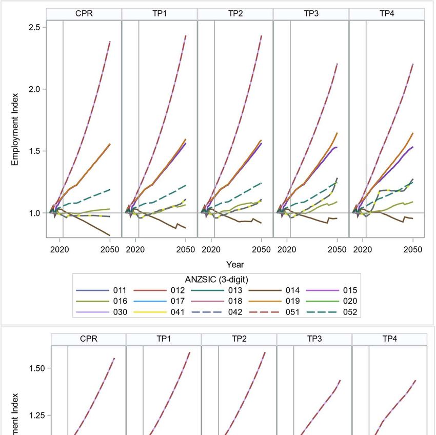
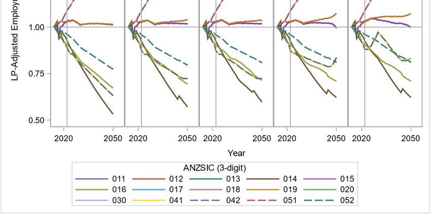
Methodology for Modelling Distributional Impacts of Emissions Budgets on Employment in New Zealand

Industrial Classification (ANZSIC06) codes to match Statistics New Zealand business and
employment data. The ANZSIC06 codes and the corresponding C-PLAN sectors are shown in the
Appendix.
 Since the employment indices from C-PLAN include changes in labour productivity and
since we wanted to isolate the employment changes related to workers, we adjusted the
employment indices by removing the labour productivity (LP) component using the same growth
rate originally used in C-PLAN. For the draft advice, the growth rate used in the modelling was
1.2% annually for all sectors. For the final advice, this was adjusted to 1% to align with general
government climate projections and with the Fiscal Strategy Model Projections. In DIM-E, this is
a macro variable to allow for easy adjustment of the rate.
 As an example, Figure 1 shows the employment indices used in the draft advice for
industries in Agriculture, Forestry, and Fishing (A)28 from C-PLAN which include changes from LP
(top panel) and with LP removed (bottom panel). Under the CPR and each TP, we can see that
Forestry and Logging (A030) and Forestry Support Services (A051) are expected to grow (both
before and after adjusting for LP) between 2022 and 2050. Sheep, Beef Cattle and Grain Farming
(A014), on the other hand, is expected to decline between 2022 and 2050 under the CPR as well
as under all four transition pathways both before and after adjusting for LP; however, the
decline is more pronounced after adjusting for LP.
 DIME-E then estimates annual employment (in terms of worker-job equivalents) over the
time period starting with the base year to the end of the projection (2014-2050 for our analysis)
under each scenario (i.e., the CPR and each TP) by multiplying the LP-adjusted employment
indices by the number of worker-jobs in each ANZSIC06 industry29 in the base year (2014). Our
base year estimates are from the LEED from Statistics NZ30. DIM-E then uses these annual
employment numbers to assess the year-over-year changes in worker-job equivalents (“WJEs”)
under each scenario for each ANZSIC06 industry. From year-to-year, an industry might grow,
contract, or stay the same size in terms of WJEs, and this may be different across the different
scenarios. If the year-over-year change was positive (i.e., an industry in 2016 has more jobs than
in 2015), DIM-E counts this change as WJEs gained. Conversely, If the year-over-year change was
negative (i.e., an industry in 2016 has fewer jobs than in 2015), DIM-E counts the change as WJEs
lost.

28 When we discuss a specific ANZSIC06 industry, we will include the corresponding ANZSIC06 code in parentheses.
29 A description of each industry, as well as the corresponding ANZSIC06 code, is provided in the Appendix.
30 See Section 3 for more detail about the data used.

 10

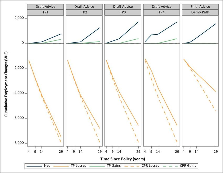
Methodology for Modelling Distributional Impacts of Emissions Budgets on Employment in New Zealand

 Next, DIM-E compares the number of WJEs gained (“gains”) and WJEs lost (“losses”) under
each transition pathway to those gained or lost under the CPR to calculate the net gains, net
losses, and overall net change (“net”) in each year for each transition pathway:
 = − 
 = − 
 = − 
where indicates the transition pathway.
 The net changes are then summed over the specified time periods, and these time periods
can be flexibly specified as macro variables in DIM-E.31 In the initial case, these time periods
aligned with the CCC’s budget cycles: 4 years, 9 years, 14 years, and 29 years after
implementation (with 2022 being the first year where effects are observed). This allowed us to
evaluate the cumulative effects of each transition pathway at multiple points in time over the
forecast period (2022-2050). As an example, we show the cumulative employment changes in
Sheep, Beef Cattle and Grain Farming – which we hereafter call Sheep/Beef (A014) – in Figure 2.
Each panel in the figure shows the cumulative gains (green lines) and losses (orange lines) for
each policy scenario (i.e., each pathway) relative to its reference scenario (e.g., CPR). The solid
lines represent the predicted employment changes under the pathway scenarios, and the
dashed lines represent the predicted employment changes under the reference scenarios.32
 In Figure 2, one can quickly see that substantial losses are predicted for the industry in all
scenarios, that these losses are expected to be less under each pathway relative to its CPR by the
end of the forecast period, and that the net differences vary across the pathways. From Figure 2,
we also see some gains are predicted under the transition pathways used for the draft advice
over the last period (but not under the CPRs) and that the overall net effects (dark blue lines) of
the transition pathways combines these gains with fewer losses to achieve an overall net
positive effect for this industry by the end of the forecast period. It is also important to highlight
that the cumulative net positive effect indicates that the industry is expected to have more WJEs
at the end of the period under the pathways than would be the case under the CPRs. However,
this does not mean that the industry is expected to end the forecast period with more jobs.
Clearly, this industry is expected to decline between 2014 and 2050 – by almost 50% as shown in
Figure 1 under the CPR and slightly less so under the four pathways.

31 DIM-E was constructed using SAS software. Copyright ©2019-2020, Institute Inc. SAS and all other SAS Institute Inc.
product or service names are registered trademarks or trademarks of SAS Institute Inc., Cary, NC, USA. SAS and all other SAS
Institute Inc. product or service names are registered trademarks or trademarks of SAS Institute Inc. in the USA and other
countries. ® indicates USA registration.
32 For the draft advice, the same reference scenario was used for each transition pathway; however, the reference scenario

was updated for developing the final advice. This can be seen by the differences in the dashed lines between the draft
advice panels and the final advice panels.
 11

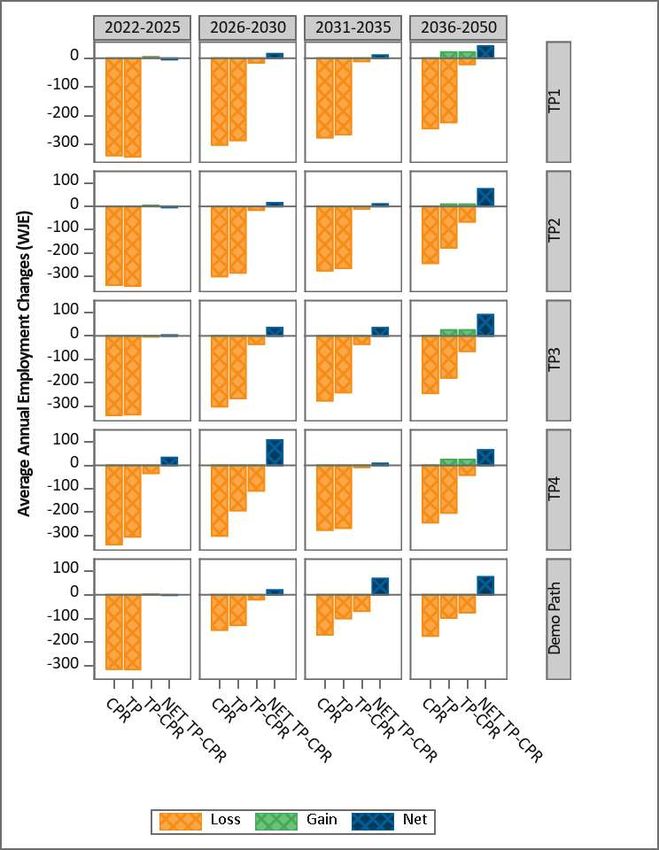
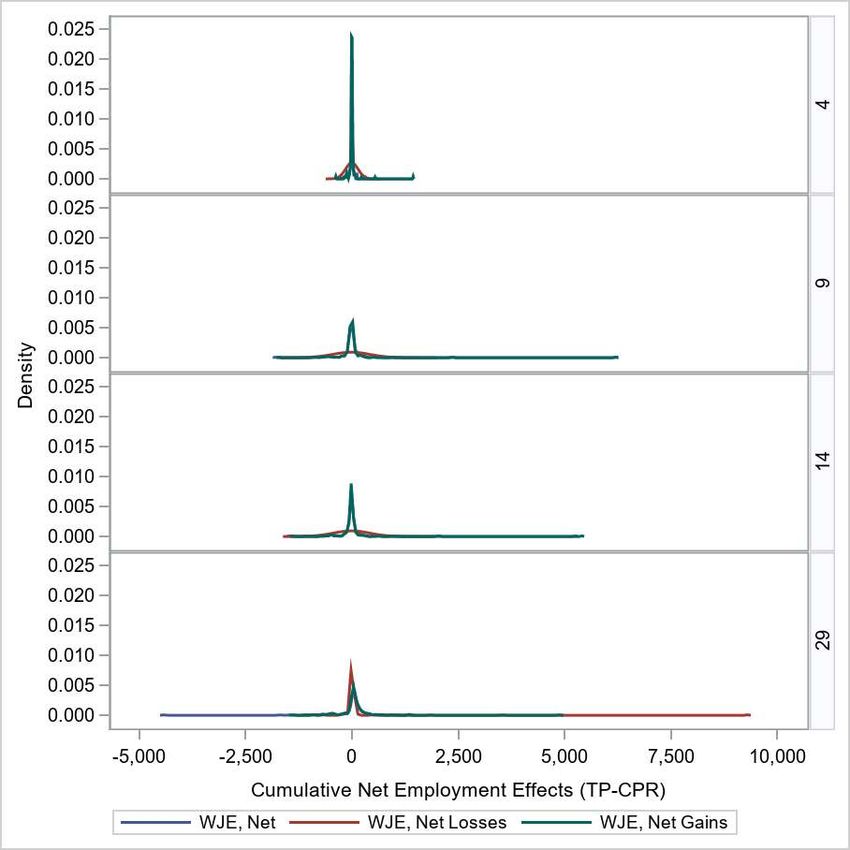
Methodology for Modelling Distributional Impacts of Emissions Budgets on Employment in New Zealand

 While it is possible to evaluate the year-to-year effects given that we have annual data, the
annual predictions from the model are likely to be lumpier (i.e., large changes from year-to-year)
than the changes would actually be in reality and subject to more error caused by short-term
fluctuations. As can be seen in the bottom panel Figure 1, there are some sharp changes in the
LP-adjusted employment indices under the transition pathways which indicate sharp changes in
annual employment levels. Therefore, examining the cumulative effects is more meaningful than
examining the annual changes. (Chen et al., 2016)
 Moreover, we can still examine the predicted annual effects by estimating the average
annual effects during each time period. These results are shown in Figure 3 where we once again
use Sheep/Beef (A014) as our example industry. In the figure, losses are again shown in orange,
gains are shown in green, and the net effects are shown in blue. This figure is complementary to
Figure 2 but provides a better view of the timing of gains and losses and an easier comparison of
the average annual difference between the pathway and its CPR. In the case of Sheep/Beef
(A014), it shows that the largest losses are predicted to occur between 2022 and 2025 and that
there are very small differences between the losses expected under the pathways and the CPRs.
 Aggregating results over longer time periods smooths shorter-term fluctuations in the
predicted effects, which should provide more robust results. Even so, the timing of the results
may not happen exactly as predicted. However, sensitivity analyses could be used to examine
the effect the time period selection has on the average cumulative effects, which can be easily
done by using the flexible time period specification that DIM-E provides.
 Using DIM-E, we can also assess the distribution of industries over net employment effects
for each cumulative time period as shown in Figure 4 and Figure 5. These figures can also be
used to examine how the distributions of these effects change as time passes. In Figure 4 and
Figure 5, we used publicly available LEED data for the kernel density estimates, and hence, these
results are very likely to differ from the results using the non-public LEED data that was used in
Riggs & Mitchell (2021). We provide these results as representative of the types of results that
can be obtained using data from DIM-E, but these results are for demonstration purposes only.
 In Figure 4, we can see that the industry-level net effects under TP4 spread out over time.
We can also see that after 4 years a large number of industries have zero net gains (green line)
under TP4 compared to the CPR and that there are far fewer industries with zero net losses (red
line). Moreover, we can see that after nine years the density of industries with net gains around
zero under TP4 reduces substantially, and after 29 years, the density of industries with net gains
is actually surpassed by the density of industries with net losses. Hence, we can conclude from

 12

Methodology for Modelling Distributional Impacts of Emissions Budgets on Employment in New Zealand

this that after the first period, most affected industries that are affected by losses but over time
about the same number of industries are affected by gains and by losses.
 To see the implications for the total net effects, we separately show these for TP4 in Figure
5. Given the similarity in the distributions between the net gains shown in Figure 4 and those
shown for the total net effects shown in Figure 5, especially in the first three periods, it appears
that the distribution of net effects is largely reflective of the distribution in net gains in this
example. The exception may be the long, left tail seen in the total net effects distribution over
the whole time period (over 29 years) which reflects the long right tail seen in the distribution of
net losses in Figure 4. Using distributions in this manner provides insights into the extent to
which the effects of the policy will be felt across the economy and how this may change over
time.
 The next step in DIM-E is to use these net changes to rank each industry under each
transition pathway in terms of those with net positive changes ( > 0) and in terms of
those with net negative changes ( < 0) during a given time period. As mentioned
previously, a net positive change indicates that the industry will have more jobs under the
transition pathway than under the CPR; however, this does not mean that the industry will grow
during the time period. It is possible for an industry to lose jobs over the time period under both
the transition pathway and under the CPR – a net positive change for the industry in this case
indicates that the industry is expected to lose fewer jobs under the transition pathway than
under the CPR. Similarly, a growing industry can have a net negative change which indicates that
the industry is growing less under the transition pathway than under the CPR. Moreover, in a
given time period, an industry can both grow and contract – the net effect depends on whether
the industry ends up with more or less jobs under the transition pathway than under the CPR.
 In Table 2 and Table 3, we show these rankings for the cumulative net effects over the full
forecast period (2022-2050). Table 2 shows the industries with the largest net positive effects
under each pathway. From this table, we can see that the results are fairly consistent across all
of the pathways, with Air and Space Transport (I490) ranked first in 4 out of 5. From this table,
we can also compare the relative net effects across the pathways. For example, the net effects
for Air and Space Transport (I490) under TP1 and TP2 are fairly similar (967 WJE under TP1 and
956 under TP2) and that the net effects under TP3 (1,995) and TP4 (2,076) would be almost
double.
 Table 3 shows the industries with the largest net positive effects under each pathway.
On the net negative side, the industries are not as consistently ranked across the pathways as
they are on the net positive side. For example, Other Machinery and Equipment Manufacturing

 13

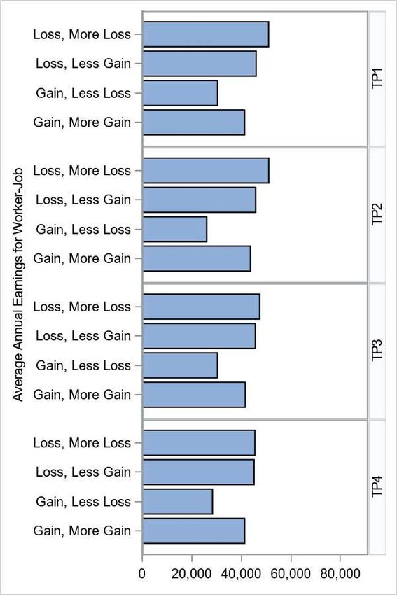
Methodology for Modelling Distributional Impacts of Emissions Budgets on Employment in New Zealand

(C249) is ranked first under TP1 (-606 WJE) and TP2 (-645), but Road Freight Transport (I461) is
ranked first under TP3 (-1,835 WJE) and TP4 (-2,181 WJE). Still, the relative magnitudes across
the pathways are still similar when looking across ranks.
 To better understand these changes, we categorise the net effects into four types:
  Gain-Less Loss: these are net positive changes due to fewer jobs lost under the transition
 pathway than under the CPR;
  Gain-More Gain: these are net positive changes due to more jobs gained under the
 transition pathway than under the CPR;
  Loss-Less Gain: these are net negative changes due to fewer jobs gained under the
 transition pathway than under the CPR; or
  Loss-More Loss: these are net negative changes due to more jobs lost under the
 transition pathway than under the CPR.
 In Sheep/Beef (A014), we can see these different net effects in Figure 3. For example,
under TP1 and TP2 in the first time period (2022-2025), we can see that the industry has more
losses under the pathway than under the CPR, and hence, these net negative effects would be
counted as “Loss-More Loss”. On the other hand, under TP3, we can see that the industry has
fewer losses during the same time period compared to the CPR, resulting in a net positive effect
for the pathway (or a “gain” for the pathway over the CPR). However, this gain is not resulting
from growth in the industry but from less decline. For this reason, we would label this net effect
as “Gain-Less Loss”. In the final period, we see some growth in the industry and some decline in
the industry under all pathways, and there is more growth and less decline under the pathways
compared to the CPR. Hence, there are gains to the economy from the pathway (relative to the
CPR) from both more jobs gained and from fewer jobs lost, and DIM-E distinguishes these effects
as “Gain-More Gain” and “Gain-Less Loss” because while these effects may be mathematically
equivalent, they may not be functionally equivalent in actual application.
 It is important to understand that these simulation models are designed to examine how
various aspects of the economy are likely to change due to different economic or policy
conditions (Chen et al., 2016), and any of the DIM-E results must be interpreted carefully,
drawing on the scenario details and the outputs from the C-PLAN model. Moreover, a key
strength of this type of analysis is in the ability to assess the net effects of different policy
decisions relative to the baseline scenario.

 14

Methodology for Modelling Distributional Impacts of Emissions Budgets on Employment in New Zealand

1.3 Simulation of Worker-Job Characteristics
To better understand the types of workers that are expected to be affected under each
transition pathway, DIM-E uses the net change in worker-jobs for each of the four time periods
(4-, 9-, 14-, and 29-years post-implementation) in each ANZSIC06 industry. DIM-E uses these
numbers as the basis for the counts of the simulated worker-jobs, with each simulated worker-
job flagged as one of the four net effect types (based on industry) as specified at the end of the
last section: Gain-Less Loss (GLL); Gain-More Gain (GMG); Loss-Less Gain (LLG); or Loss-More
Loss (LML). The counts of WJE used in the simulation in each of these four categories for the first
time period (2022-2025) are shown in the left panel of Figure 6 and for the full time period
(2022-2050) are shown in the right panel. These results show us how much reallocation or
“churn” should be expected under the different pathways and over time. For example, TP4 is
predicted to have the most churn in the first time period relative to the other pathways
considered in the draft advice, but by the end of the forecast period TP3 has almost as much
churn as TP4. In addition, TP4 has more LML than TP3 over the full time period (10,652 and
7,134 respectively), but TP4 also has more GMG than TP3 (22,408 and 17,785 respectively).
 Next, DIM-E uses the 2018 percentage of short-spell worker-jobs in each ANZSIC06
industry to simulate whether the worker-job was a short-spell worker-job and then separates
the simulated data set into short-spell and non-short-spell worker-jobs. This is done to simulate
the characteristics for each worker-job using separate profiles for short-spell and non-short-spell
worker-jobs in each ANZSIC06 industry from the 2018 worker-jobs data.33
 The simulation was done using SAS software34 -- specifically, DIM-E uses the RAND
function to simulate characteristics of the worker and the job for each worker-job. The RAND
function uses the Mersenne-Twister random number generator developed by Matsumoto &
Nishimura (1998) and can generate random numbers from a variety of different distributions.
(Wicklin, 2013, 2015) DIM-E primarily uses the Table and Bernoulli distributions, though the
Normal distribution is also used for simulating annual earnings for the worker-jobs using the
mean and standard deviation for the ANZSIC06 industry and restricting the values to be between
the industry’s minimum and maximum values because this provided a more reasonable
approximation of earnings in the simulation. The simulation is run 1000 times (though this is

33 A number of industries, especially agricultural industries, use a number of short-spell workers, and the characteristics of
worker-jobs are often very different for short-spell and non-short-spell worker-jobs.
34 Copyright © 2019-2020, SAS Institute Inc.

 15

Methodology for Modelling Distributional Impacts of Emissions Budgets on Employment in New Zealand

flexibly specified using a macro variable) and the sample mean for each characteristic is
calculated.35
 For characteristics of workers holding these jobs, DIM-E simulates workers’ gender, age,
highest qualification, and ethnicity. For characteristics of the jobs themselves, DIM-E simulates
average annual earnings (in 2018 NZD), region, and whether the worker-job was a continuer 36.
For workers’ ages, the simulation was based on the percentage of workers in each age group in
each ANZSIC06 industry rather than on the continuous distribution of worker age because using
age groups provided a more accurate approximation of the different profiles of worker-jobs for
our industries. For average annual earnings, we used a minimum and maximum value based on
the distribution of earnings in each ANZSIC06 industry.
 While we have actual values for the characteristics of workers in the affected industries,
the simulation allows us to go beyond industry classifications to examine the cumulative net
effects of the policy scenarios on different groups of workers across New Zealand and in
different regions.

4. Sample of Results from DIM-E Worker-Job Simulation
The following section provides a sampling of results from the DIM-E simulation of worker-jobs to
illustrate the different ways in which DIM-E can be used. There are far more results that could
be produced from DIM-E, with many of our main results presented in Riggs & Mitchell (2021).
Many of these results are shown as percentages of the affected jobs. To calculate these
percentages, we estimated the total number of worker-jobs affected either in a positive or
negative way under the pathway and then estimate the percentage of worker-jobs in each group
from the total number affected. For example, if 100 women are in worker-jobs expected to be
negatively affected under a given transition pathway and 100 men are in worker-jobs expected
to be positively affected, then the total number of affected worker-jobs is 200 and the
percentage of worker-jobs affected for women would be -50% (negative to represent the
negative direction) and 50% for men (positive to represent the positive direction). We can then
compare the percentage of affected worker-jobs for the group to the percentage of all worker-
jobs held by the group in 2018. Hence, we can see if some groups are disproportionately
affected by the changes.

35 We compared the sample means from the simulation (based on the profiles for short-spell and non-short-spell worker-
jobs) to the overall profile of all worker-jobs in a sample of industries, and the simulated sample means were close
approximations of the overall worker-job profile for the industries.
36 Continuers apply only to non-short-spell jobs only since short-spell jobs, by definition, are not continuers.

 16

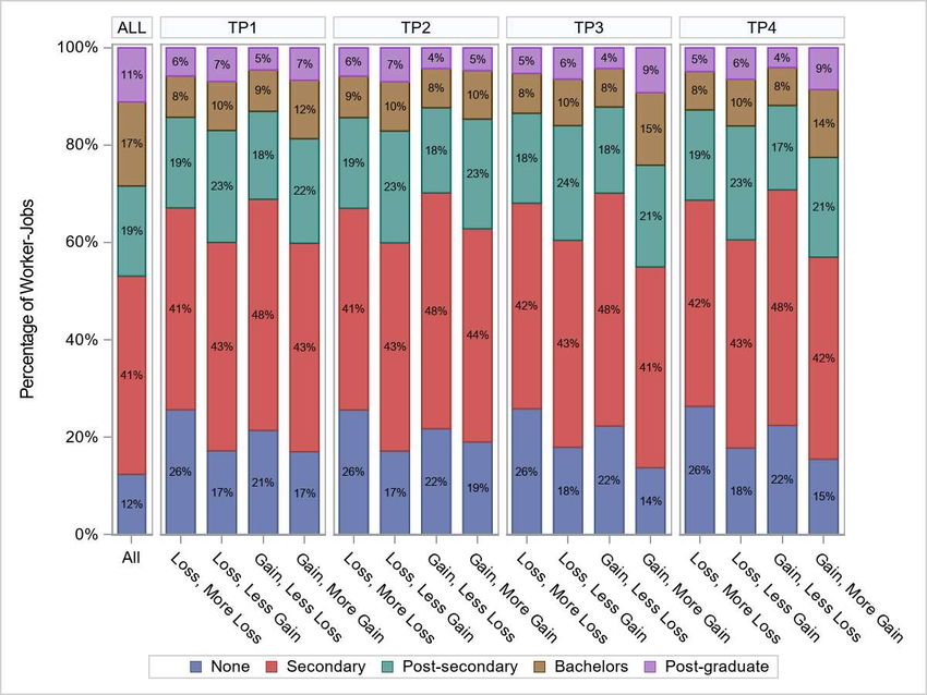
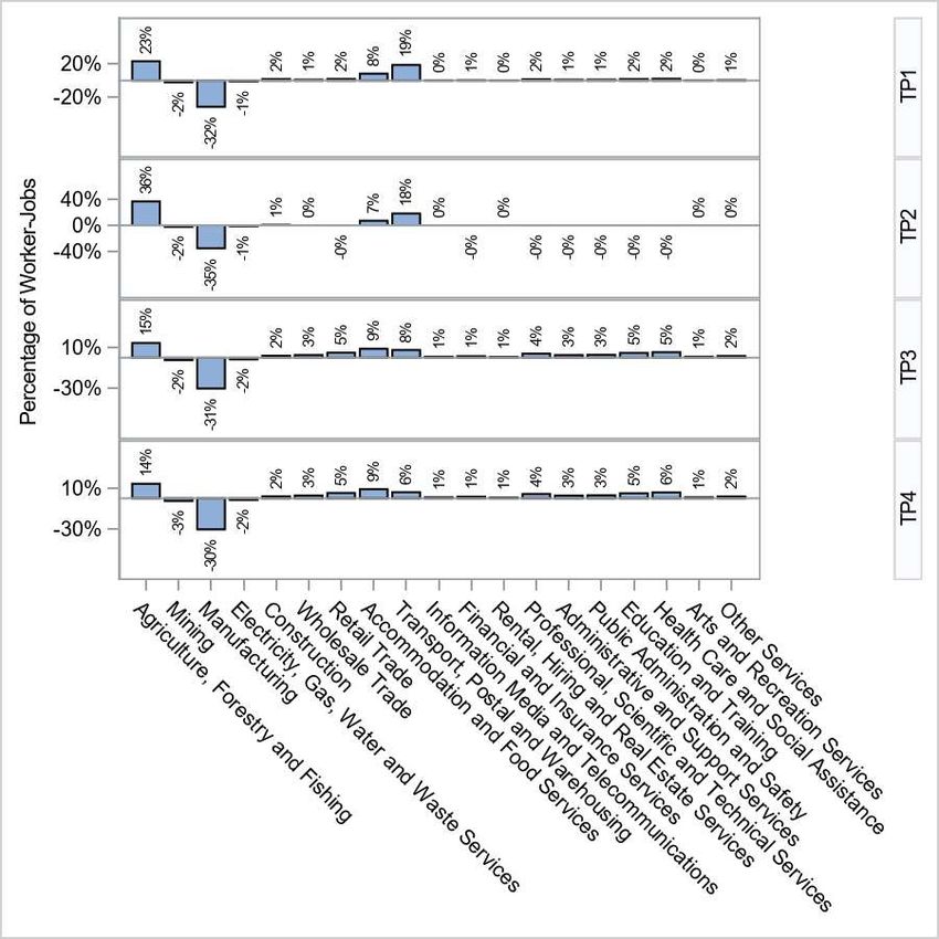
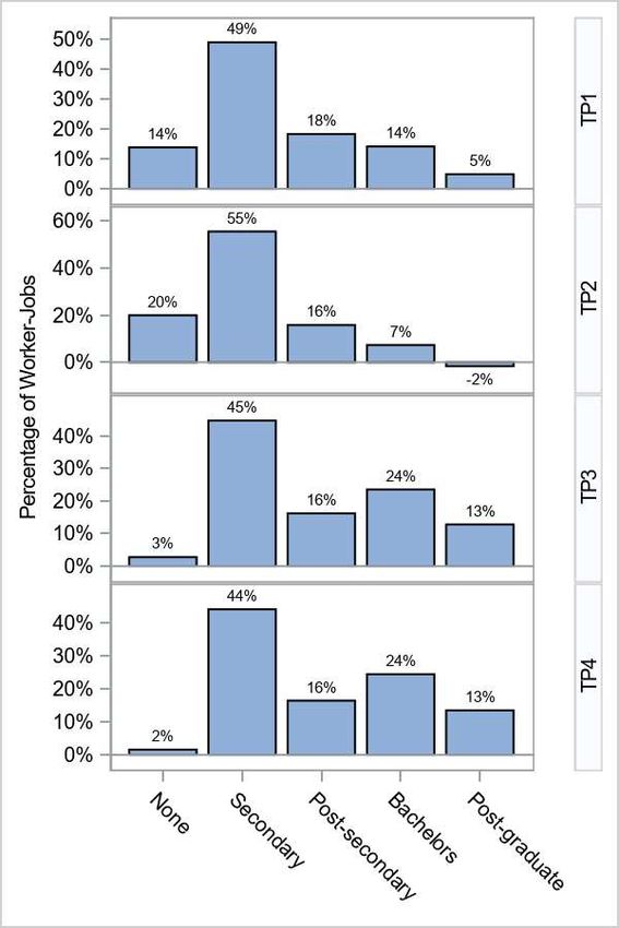
Methodology for Modelling Distributional Impacts of Emissions Budgets on Employment in New Zealand

 We begin with the results for earnings by net effect type as shown in Figure 7. The left
panel of Figure 7 shows average annual earnings for the first period (2022-2025), and we can see
that the average annual earnings for worker-jobs in all categories under all four pathways
(between $40-$50,000) are fairly similar with the exception of jobs in the LML category under
TP4. The average for this category exceeds $80,000. Hence, under TP4, the jobs where more
losses are expected under the pathway are relatively well paid. By 2050, however, average
annual earnings in the LML category are similar to those seen in the other categories (results in
right panel of Figure 7). It is of note that worker-jobs in the GLL category appear to average less
than worker-jobs in the other categories under all four pathways. Hence, WJE gained from
industries that decline less than they would have otherwise under the CPR are less well-paid
than WJE in the other categories.
 It is important to note that earnings will vary over the forecast period due to inflation and
changes in supply and demand; however, these estimates do not account for those changes. This
analysis still provides an indication of the relative earnings across different net effect types as
those are less likely to change especially in the short and medium term.
 DIM-E can also be used to examine the proportional changes across broader industries
categories which include all industries and not just the industries with the largest changes (as we
had with the industry rankings). Figure 8 shows share of net effects for one-digit ANZSIC06
categories over the full forecast period (2022-2050). From this, we can see that the net effects
for most of these broad industry groupings will be small. Manufacturing (C) is predicted to have
the largest share of affected worker-jobs under almost every pathway, and the direction is
always negative (ranging from -30% to -35% depending on the pathway). Only two other broad
industries consistently have net negative effects over the full forecast period under all four
pathways: 1) Mining (B) and 2) Electricity, Gas, Water and Waste Services (D). However, the
shares for these industries are small (between -1% and -3% in all cases). On the positive side,
Agriculture, Forestry, and Fishing (A) is expected to have a large share of affected worker-jobs
under all four pathways (ranging from 14% to 36%).
 Using the DIM-E simulation of worker-jobs, we can also examine the aggregate effects of
these changes for different groups of workers. As an example, we present the results for
workers based on their highest qualification with net effects aggregated over the full forecast
period (2022-2050) as shown in Figure 9. These results indicate that each group of workers is
expected to have a net positive share of the effects at the end of the forecast period under all
four transition pathways. The one exception is post-graduate workers under TP2 who are
expected to have a net share of approximately -2%. This indicates that for each category of

 17