How does the control logic influence the establishment of a data-driven chiller model?

Journal of Physics: Conference Series

PAPER • OPEN ACCESS

How does the control logic influence the establishment of a data-driven
chiller model?
To cite this article: Shunian Qiu et al 2021 J. Phys.: Conf. Ser. 2006 012002

View the article online for updates and enhancements.

 This content was downloaded from IP address 46.4.80.155 on 18/09/2021 at 07:44

CRSA 2021 IOP Publishing
Journal of Physics: Conference Series 2006 (2021) 012002 doi:10.1088/1742-6596/2006/1/012002

How does the control logic influence the establishment of a
data-driven chiller model?

 Shunian Qiu1, Zhenhai Li1, Ruikai He1, Jiajie Li2 and Zhengwei Li1, 3*
 1
 School of Mechanical Engineering, Tongji University, Shanghai, Shanghai, 201804,
 China
 2
 China Academy of Building Research, Beijing, Beijing, 100013, China
 3
 Key Laboratory of Performance Evolution and Control for Engineering Structures of
 Ministry of Education, Tongji University, Shanghai, Shanghai, 201804, China
 *
 Corresponding author’s e-mail: zhengwei_li@tongji.edu.cn

 Abstract. The modelling of chiller performance is critical for chiller optimal control, and fault
 detection and diagnosis (FDD). Different kinds of chiller models including sophisticated
 mechanistic models (white-box models), purely data-driven models (black-box models like
 artificial neural networks, ANN), and semi-physical models (grey-box models like empirical
 equations) have been proposed and tested. Due to the development of machine learning
 techniques, data-driven models have become more popular recently. The performance of the
 established data-driven model (accuracy, robustness, generalization) could significantly affect
 the model application. To enhance the model performance, a lot of studies have been carried out
 on investigating and modifying the model structure. However, the influence of the data quality
 on model training has not been sufficiently studied. When adopting historical data to train models,
 the data distribution is highly correlated to the control logic. So how does the control logic
 influence the establishment of data-driven chiller models by affecting the data distribution? In
 this study, experiments are conducted on an air-cooled chiller under model-free stochastic control
 to acquire rich and variable operational dataset; then the dataset is grouped into three
 corresponding to different chiller control logics. Finally, three models trained by three training
 datasets are evaluated, and the results suggest that when establishing data-driven chiller models,
 preliminary stochastic operation is cost-effective to acquire rich data for robust chiller modelling.

1. Introduction
In the operation and maintenance of building HVAC systems, the modelling of chiller performance is
critical for model-based chiller optimal control and chiller fault detection and diagnosis (FDD). With an
established chiller performance model, the chiller power and COP could be estimated with given input
variables including chilled water temperature, cooling water (condenser water) temperature, and chiller
cooling load.
 In order to modelling the chiller performance, different kinds of chiller performance models were
proposed, evaluated and validated. Chiller models could be categorized into three types: models based
on physical mechanisms (white box models), pure data-driven models (black-box models like random
forest, artificial neural networks), and semi-physical models which consider physical mechanisms in
chillers’ working cycle but still require operational data to determine the model coefficients. Specifically,
selected data-driven model frameworks are listed in Table 1.

 Content from this work may be used under the terms of the Creative Commons Attribution 3.0 licence. Any further distribution
 of this work must maintain attribution to the author(s) and the title of the work, journal citation and DOI.
Published under licence by IOP Publishing Ltd 1

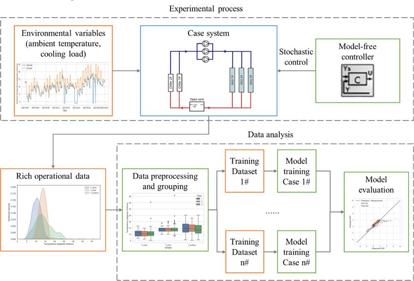
CRSA 2021 IOP Publishing
Journal of Physics: Conference Series 2006 (2021) 012002 doi:10.1088/1742-6596/2006/1/012002

 The application of data-driven models typically includes three steps: (1) Collect equipment operation
data (historical data or experimental data); (2) train a model framework with the collected data to
determine the model coefficients; (3) utilize the established model in the online optimal control or FDD.
 Table 1 Selected review of existing chiller models.
 Output
References Input variables Model framework a
 variable

 Polynomial equation
 [1-4] 
 
 , , , 
 [5] , , , 
 , , , 

 Simplified Multivariate Polynomial model (SMP model)
 [6, 7] , , 
 
 Gordon-Ng model
 1
 [8] , , 1 1 
 1 1 
 ∙ 
 Multivariate Polynomial model (MP model)
 [8, 9] , , 
 
 VT model
 [8] 
 
 log 
 a
 —Chiller input electrical power (kW)
 CL—Chiller cooling load (kW)
 PLR—Chiller partial load ratio
 COP—Chiller coefficient of performance
 —Chilled water flowrate (m³/h)
 —Chilled water return temperature (℃)
 —Chilled water supply temperature (℃)
 —Outdoor air temperature (℃)
 —Condenser water return temperature (℃)
 It could be seen that all the selected model frameworks contain coefficients ( ) to be determined,
and typically they are determined with chiller operational data regression. In order to enhance the model
accuracy, three approaches are available: improve model framework, improve the solver (optimizer)
used in the regression procedure, improve the quality of the data for regression. Swider [9] compared
the performance of different chiller model frameworks (linear model, multivariate polynomial model,
bi-quadratic model, artificial neural network, etc.) with one operation data sample. Reddy and Anderson
[8] analysed the influence of regression solvers (ordinary least squares, ridge) on the model estimation
accuracy. They also investigated the model accuracy under different training/testing dataset (sequential
dataset and extreme dataset).
 When historical operational data is used for regression, the former control strategy of chillers could
influence the historical data distribution and furtherly, the establishment of chiller models. Hence, in
this study, it is investigated how the control logic influences the data-driven chiller modelling.

2. Workflow overview
The workflow of this study is illustrated in Figure 1:

 2

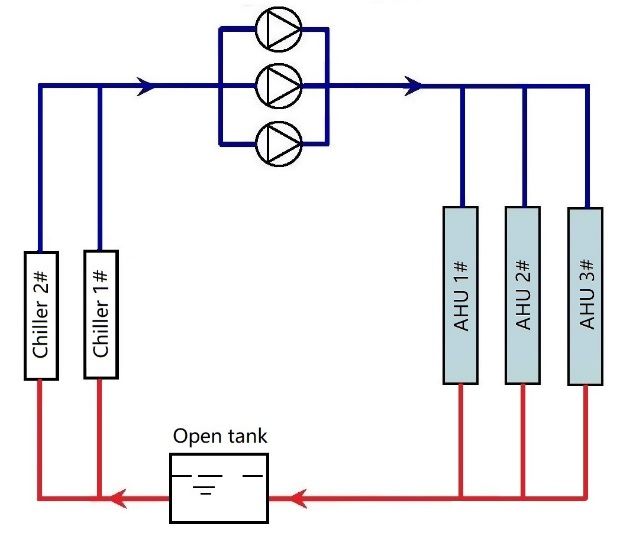
CRSA 2021 IOP Publishing
Journal of Physics: Conference Series 2006 (2021) 012002 doi:10.1088/1742-6596/2006/1/012002

 1. Operation experiments are implemented to an air-cooled chiller under model-free stochastic
control to acquire rich operational data including chilled water supply temperature ( ), chilled water
return temperature ( ), chilled water flowrate ( ), outdoor air temperature ( ), the
setpoint of chilled water supply temperature ( , ), and chiller electrical input power (P).
 2. Pre-process the original data, group the pre-processed data with certain rules to generate datasets
corresponding to different chiller control logics. For instance, selecting the data items where ,
equals 8 ℃ generates the chiller operational dataset corresponding to a constant control logic
(conventional chiller operation strategy in most buildings).
 3. Train a common chiller model framework with generated datasets corresponding to different
control logics.
 4. Evaluate the performance of models trained with different datasets.

 Figure 1 Workflow of this study.

3. Experimental case study

3.1. Case system
The air-conditioning system in a factory building in Jiangsu province is adopted as the experimental
case system. The system is composed of two air source heat pumps, three identical chilled water pumps,
three air handling units (AHUs) and one open chilled water tank. The characteristics of the equipment
above are listed in Table 2. The layout of the system is illustrated in Figure 2. It should be noted that the
open water tank is designated to cool the returned chilled water with outdoor air (free cooling), this
design would cause the gap between system cooling load and chiller cooling load. In this study, when it
comes to “cooling load”, the chiller cooling load is the studied variable.

 3

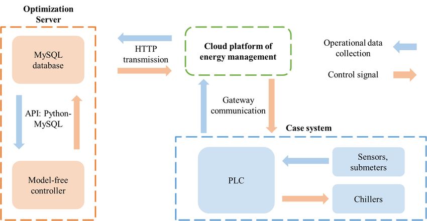
CRSA 2021 IOP Publishing
Journal of Physics: Conference Series 2006 (2021) 012002 doi:10.1088/1742-6596/2006/1/012002

 Table 2 Characteristics of the case system.
 Equipment Number Nominal characteristics
 Big: COP = 3.57, Cooling capacity = 785 kW, Input power = 220 kW,
 Screw air source Variable speed, = 7 ℃ (could be adjusted from 4 to 18 ℃)
 1 big, 1 small
 heat pump Small: COP = 3.50, Cooling capacity = 623 kW, Input power = 178 kW,
 Variable speed, = 7 ℃ (could be adjusted from 4 to 18 ℃)
 Chilled water
 3 Power = 15 kW, Flowrate = 126 m³/h, Head = 25 m, Variable speed
 pump
 1#: Fan power = 30.15kW, Air flow volume = 52000 m³/h,
 Cooling capacity = 205.06 kW
 2#: Fan power = 30.43kW, Air flow volume = 42000 m³/h,
 Air handling unit 3
 Cooling capacity = 162.68 kW
 3#: Fan power = 66.40kW, Air flow volume = 95000 m³/h,
 Cooling capacity = 453.11 kW

 Figure 2 Layout of the case system.

3.2. Experiments on chiller operation
In this study, Chiller 2# is selected as the experimental chiller, and the operation of Chiller 2# is
controlled over March to acquire data for the follow-up analysis. In most time of March 2021, the case
system operated at cooling mode, and the cooling load is merely dealt by Chiller 2#. Chiller 1# only
operated intermittently during 15:00 – 20:00 on March 2nd, and the whole system only operated at
heating mode during 10:30 – 11:40 on March 4th.
 Over March, a model-free control method based on reinforcement learning (RL) was implemented
to control the chilled water supply temperature of Chiller 2# ( , ) within (6, 7, 8, 9, 10 ℃). This
model-free controller is intended to explore and learn from the real environment to achieve energy
conservation, and in the beginning of the application (March), the control is still pretty stochastic, which
could enhance the richness of the chiller operational data. Figure 3 shows the data flow of the model-
free control implementation. Table 3 shows the format of the acquired operational data of Chiller 2#, the
control interval and data collection interval are both 10 minutes.
 Table 3 Example of the operational data under stochastic control.
 Heating/Cooling mode
 On/Off , Power 
 Time (0: Cooling, 1:
 ℃ ℃ status ℃ ℃ (kW) m³/h
 Heating)
 2021-03-01
 17.5 17.6 1 0 10 12.7 0.952 70.75
 00:00:00

 4

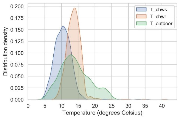
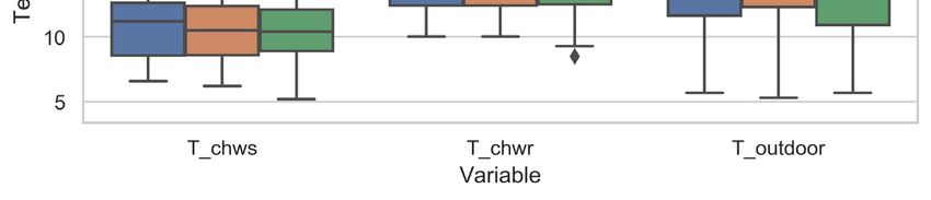
CRSA 2021 IOP Publishing
Journal of Physics: Conference Series 2006 (2021) 012002 doi:10.1088/1742-6596/2006/1/012002

 Figure 3 Data transmission procedure.

4. Data processing

4.1. Data pre-processing
In this study, the data pre-processing procedure is pretty simple. Data items with chiller input power less
than 20% of the nominal power are dropped since the compressor may not work at these time steps.
After the data cleaning, 1132 data points remained. Then, chiller cooling load (CL) and chiller COP are
calculated using equations (1) and (2) [10]:
 (1)
 (2)
where is the chiller cooling load (kW), is the specific thermal capacity of water (kJ ∙ kg ∙ K ),
 is the measured chilled water flowrate (m³/h), is chilled water return temperature (℃), 
is the water density (kg/m³), is chilled water supply temperature (℃), P is the input electrical
power of the chiller (kW).
 Figure 4 indicates that the chilled water temperature distribution is pretty wide, which could validate
the effectiveness of the model-free stochastic control in generating operational data of high richness.

 Figure 4 Temperature distributions.

4.2. Data grouping
In order to analyze how the control logic could influence the operational data distribution and chiller
modelling, the pre-processed operational data is grouped into three training datasets corresponding to

 5

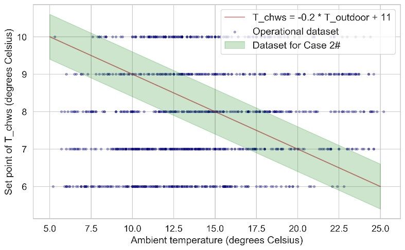
CRSA 2021 IOP Publishing
Journal of Physics: Conference Series 2006 (2021) 012002 doi:10.1088/1742-6596/2006/1/012002

three control logics: (1) constant control logic; (2) variable control logic based on outdoor
temperature ( , is adjusted by on-site operator to save chiller energy); (3) stochastic control logic
intended for rich data and robust chiller modelling.
 For the first case, the data items with , equaling to 8 ℃ (the median of the control
range) are selected as the training dataset. The quantity of the training dataset is 231.
 For Case 2#, data items where , and are close to negative linear correlation are
selected as the training dataset, the specific threshold is described with equation (3):
 , , 0.2 11
 (3)
 0.6 , , , 0.6
where , , is the exact setpoint value of when is simply controlled based on
ambient temperature; all data items matching equation (3) would be included in the training dataset of
Case 2#. The selection of training data for Case 2# is illustrated in Figure 5, where blue data points
covered by the green shadow are selected. The quantity of the training dataset is 235. Note, the threshold
in equation (3) is set to 0.6 in order to guarantee the training set quantity of Case 2# is close to that of
Case 1#; in doing so, the influence of data size on model training won’t affect the case comparison.
 For Case 3#, 231 data items are randomly sampled from the preprocessed dataset as the training set.
 And it should be noted that all three cases use the rest of the preprocessed dataset (apart from their
training set, respectively) as the test set. The data quantity of each case is addressed in Table 4; the data
distributions of each case are illustrated in Figure 6. Covariance matrixes listed in Table 4 indicate that
in all three cases, the variance of is larger than that of , and the variance of is the
smallest. Moreover, variances of and of Case 3# are evidently larger than those of the
other two cases, which verifies the effect of model-free stochastic controller.
 Table 4 Description of three training datasets.
 Covariance matrix
 Case No. , Training set quantity Test set quantity Dataset quantity
 ( , , )
 5.23 3.20 0.35
 1 8 231 901 1132 3.20 2.73 0.54
 0.35 0.54 22.45
 4.59 3.03 0.32
 Vary with 3.03 2.83 0.28
 2 235 897 1132
 0.32 0.28 14.10
 7.30 6.09 0.28
 3 Stochastic 231 901 1132 6.09 6.37 0.19
 0.28 0.19 19.91

 Figure 5 Training dataset selection for Case 2#.

 6

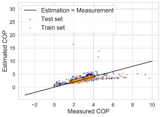
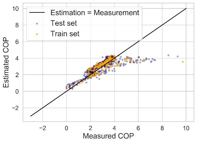
CRSA 2021 IOP Publishing
Journal of Physics: Conference Series 2006 (2021) 012002 doi:10.1088/1742-6596/2006/1/012002

 Figure 6 Data distributions of three cases.

4.3. Chiller model framework
As introduced in Section 2, the generated datasets will be used to train a common chiller model
framework. In this study, a modified version of multivariate polynomial (MP) model is adopted as the
framework. MP model is a classical data-driven chiller model which has been adopted in many studies
[8, 9]. The original MP model (equation (4)) is designed for water-cooled chillers with , , and
CL as input independent variables. Since the case chiller in this study is an air-cooled chiller, the MP
model is modified before usage in this case study (equation (5)).
 
 (4)

 (5)
 where is the cooling water (condenser water) return temperature (℃), is the outdoor
air temperature (℃), and s are coefficients determined with regression.

5. Results and discussion
The coefficient of variation of the root-mean-square error (CV(RMSE), equation (6)) is adopted as the
error indicator herein to evaluate model accuracy. The accuracy of three trained models is illustrated in
Figure 7 and Table 5.
 ∑
 ∑
 (6)
 th th
where n is the number of data points, is the i measured COP value, and is the i estimated COP
value.
 Table 5 suggests that (1) the accuracy indicator on training set is always better than test set, especially
on Case 1#; (2) the CV(RMSE) of Case 3# on test set is better than those of the other cases, which
indicates that the generalization performance of Case 3# is the best of these three. Moreover, the
operational data acquired from stochastic control is best for robust chiller modelling; (3) Although the
quantity of the training dataset of Case 3# is only 20% of the total dataset, the accuracy of model
estimation on test set is still acceptable, which infers that the operational data under stochastic control
for a short term is already OK to establish data-driven multivariate polynomial chiller models.
Figure 7 shows that when the richness of training dataset is limited (Case 1# and 2#), extreme outliers
(i.e., the data points with estimated COP over 20) may occur during the application of the trained
model, which infers unrobust generalization and application performance.

 7

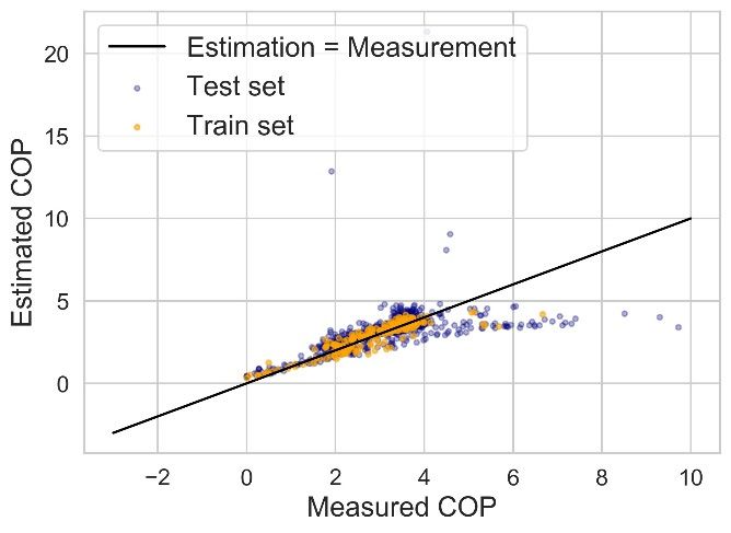
CRSA 2021 IOP Publishing
Journal of Physics: Conference Series 2006 (2021) 012002 doi:10.1088/1742-6596/2006/1/012002

 Table 5 Modelling accuracy results.
 CV(RMSE)
 Case No.
 Training set Test set
 1 14.96% 31.88%
 2 18.00% 43.41%
 3 21.61% 21.01%

 (a) Case 1# (b) Case 2#

 (c) Case 3#
 Figure 7 Modelling accuracy of three cases.

6. Conclusion
The influence of former control logic on operational data distribution and chiller modelling is analyzed
in this study. An online experiment is conducted on a real chiller in the HVAC system of a factory, under
the stochastic control of a model-free controller. The operational data of high richness is then grouped
into three training datasets corresponding to three different chiller control logics. The model training
and testing results indicate that compared to the constant control logic and -based 
control logic, the model-free controller could generate more variable training dataset, which could
enhance the accuracy, generalization, and robustness of established data-driven chiller models.
Moreover, the operational data of one week is already enough to train an MP chiller model with
acceptable accuracy. Hence, when establishing data-driven chiller models, a preliminary operation under
stochastic control is suggested to be conducted in advance to collect better data for model training; it’s
cost-effective.

 8

CRSA 2021 IOP Publishing
Journal of Physics: Conference Series 2006 (2021) 012002 doi:10.1088/1742-6596/2006/1/012002

References
[1] Lee, W. and Lin, L. (2009) Optimal chiller loading by particle swarm algorithm for reducing energy
 consumption. Applied Thermal Engineering, 29(8): 1730-1734.
[2] Chang, Y.C., Lin, J.K., and Chuang, M.H. (2005) Optimal chiller loading by genetic algorithm for
 reducing energy consumption. Energy & Buildings, 37(2): 147-155.
[3] Ardakani, A.J., Ardakani, F.F., and Hosseinian, S.H. (2008) A novel approach for optimal chiller
 loading using particle swarm optimization. Energy & Buildings, 40(12): 2177-2187.
[4] Coelho, L.d.S., Klein, C.E., Sabat, S.L., and Mariani, V.C. (2014) Optimal chiller loading for
 energy conservation using a new differential cuckoo search approach. Energy, 75: 237-243.
[5] Beghi, A., Cecchinato, L., and Rampazzo, M. (2011) A multi-phase genetic algorithm for the
 efficient management of multi-chiller systems. Energy Conversion and Management, 52(3):
 1650-1661.
[6] Cui, J. (2006) A robust fault detection and diagnosis strategy for centrifugal chillers. Hvac & R
 Research, 12(3): 407-428.
[7] Cui, J. and Wang, S. (2005) A model-based online fault detection and diagnosis strategy for
 centrifugal chiller systems. International Journal of Thermal Sciences, 44(10): 986-999.
[8] Reddy, T.A. and Andersen, K.K. (2002) An Evaluation of Classical Steady-State Off-Line Linear
 Parameter Estimation Methods Applied to Chiller Performance Data. HVAC&R Research,
 8(1): 101-124.
[9] Swider, D.J. (2003) A comparison of empirically based steady-state models for vapor-compression
 liquid chillers. Applied Thermal Engineering, 23(5): 539-556.
[10] Li, Z., Huang, G., and Sun, Y. (2014) Stochastic chiller sequencing control. Energy & Buildings,
 84(84): 203-213.

 9