Foreign Crisis Transmission to Local Labor via Exports: Evidence from the 1997 Asian Crisis - MIT Economics
←
→
Page content transcription
If your browser does not render page correctly, please read the page content below
Foreign Crisis Transmission to Local Labor via Exports:
                  Evidence from the 1997 Asian Crisis

                                           Sarah Gertler1
                                Massachusetts Institute of Technology
                                               July 14, 2021

                                                  Abstract

    This paper exploits the temporary US export drop during the 1997 Asian Crisis to demonstrate that for-
eign crises can have local labor spillovers via the export channel. I embed a Roy model into a specific-factors
setting to guide analysis, linking export fluctuations to labor markets. Empirically, traded employment fell
associated with the drop in exports to Crisis-4 countries, there was sluggish post-Crisis adjustment, and
nontraded employment in lower-education areas also fell. Using the model I estimate that short-run cross-
sector distributional heterogeneity is larger than long-run. Computational estimates find the shock lowered
1998 US traded employment by 135,000-150,000 workers. JEL Codes: F14, F16

   a
    Email: sgertler@mit.edu. I thank Dave Donaldson, David Autor, Nina Pavcnik, Douglas Staiger, Bruce Sacer-
dote, Robert Staiger, Paul Goldsmith-Pinkham, Mary Amiti, Linda Goldberg, Karthik Sastry, and participants at
the MIT trade tea for helpful comments.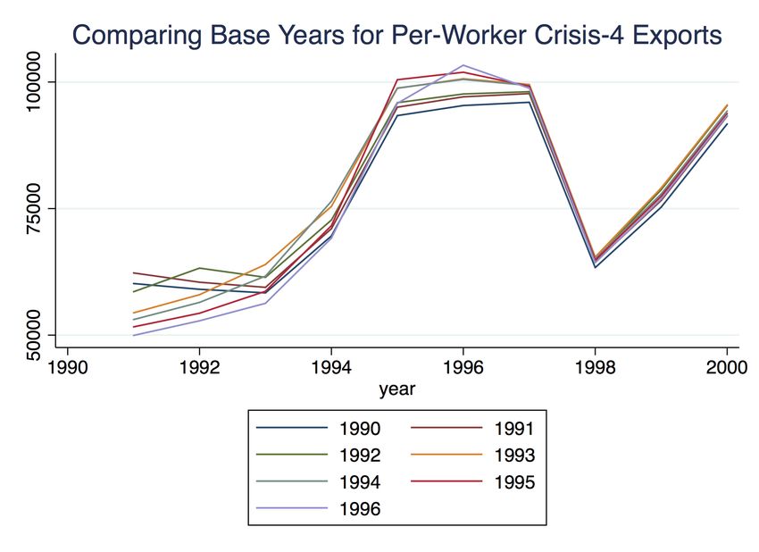
1     Introduction

    This paper demonstrates that foreign macroeconomic shocks impact local labor markets via shifts in

export demand. The estimation strategy exploits the US export drop during the Asian Crisis of 1997. A

major literature has developed that studies the effect of a change in imports on employment: Revenga (1992),

Topalova (2010), and Autor, Dorn, and Hanson (2013, 2015, 2016) are prominent examples. This work has

generally found that import penetration reduces employment. There has been relatively less work on the

effect of variation in export demand on labor market activity, though recent papers by Dauth, Findeisen,

and Suedekum (2014) and Feenstra, Ma, and Xu (2017) estimate the effect of exports on labor. Both papers

exploit gradual trade expansions. This paper builds on that literature to show that through the export

channel, economic crises in foreign countries can impact local labor markets.

    The Crisis, discussed in further detail in Section 3, was a financial crisis in a select number of Asian

countries. It occurred independently of output and employment in the US. The affected countries saw severe

drops in both exchange rates and gross domestic product (GDP) per capita. This led to a decline in import

demand in those countries, and a resulting drop in exports for a segment of US industries. Thus, the Crisis

featured a substantial US export shock.

    To estimate the Asian Crisis’s export channel transmission to US labor the paper proceeds as follows:

I develop a theoretical model based on Kovak (2013), Galle, Rodriguez-Clare, and Yi (2018), and Roy

(1951), which guides an empirical specification. The empirics employ a Bartik (1991) design, constructing

an industry-weighted commuting zone (CZ) level exposure measure of US exports to Crisis-4 (Indonesia,

Thailand, South Korea, and Malaysia) countries. Using an instrumental variables approach, the paper

exploits an analogous measure constructed using exports from five other developed countries (Australia,

Denmark, New Zealand, Spain, and Switzerland).1 This estimation design is informed by the recent shift-

share literature ((Adao, Kolesar, and Morales (2019), Borusyak, Hull, and Jaravel (2020), and Goldsmith-

Pinkham, Sorkin, and Swift (2021)).

    The main empirical estimation in Section 6 employs a stacked-log-difference empirical design, comparing

the effect of the drop in exports from 1996-1998 to the effect in the pre-period. Traded employment fell

substantially associated with the drop in exports during the Crisis. Event study estimates suggest it did not

fully recover until approximately 2003, four years after the Crisis ended. I conduct a series of robustness on

these results. There were also aggregate employment effects, and these latter effects are stronger in relatively

lower-education CZs.
   1 Autor, Dorn, and Hanson (2013) also use Finland, Germany, and Japan. I elect not to use Japan because it may have

confounding effects from the Asian Crisis. I choose the five countries because they have the most predictive power of US Crisis-4
exports.

                                                               1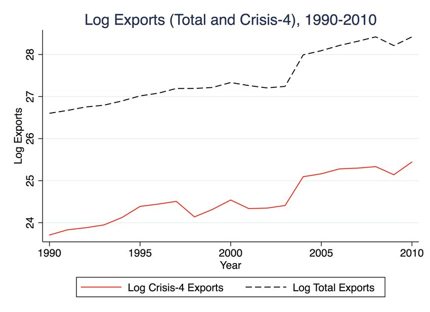
The model structure enables estimation of the degree of worker heterogeneity in the regression sample, and

considering the nature of the Asian Crisis the parameter I estimate is for the short-run. It governs how sectors

differentially respond to the Asian Crisis and can be generalized to guide expectations for heterogeneous

responses to other trade channel shocks. An additional benefit of this parameter estimation is I can compare

it to longer-run estimates in the literature to gain an understanding of how short-run adjustment differs

from the long-run. Lastly, it enables general equilibrium computation of total employment losses from the

shock. The parameter estimate demonstrates evidence for a stronger degree of worker heterogeneity, and

therefore stronger within-CZ distributional consequences of a trade shock, in the short-run relative to the

long-run. Armed with this parameter, I use the structure of my model to quantify the general equilibrium

effects of the shock. Consistent with initial empirical work, traded employment was between 135,000 and

150,000 workers fewer across the US (between 190-210 per CZ) associated with the shock.

     The paper is structured as follows. The next section discusses existing literature. Section 3 provides

background on the Asian Crisis of 1997 and discusses my measurement of exposure to the Crisis, and Section

4 contains the theoretical design. Data discussion, empirical design, and results follow. I then structurally

estimate the short-run heterogeneity parameter and use it to compute general equilibrium effects of the

shock. Section 8 contains concluding remarks and suggestions for further research.

2      Background Literature

     This paper follows from an extensive literature regarding the relationship between trade and employment.

This link has been explored across countries, industries, industries within a country, and regional labor

markets within a country. I focus on the literature that explores regional labor market effects.

     The literature in recent years has been spearheaded by a series of papers on rising Chinese import

penetration by Autor, Dorn, and Hanson (2013, 2015, and 2016).2 In their flagship paper, the authors find

that Chinese import penetration reduced US employment over the period 1990-2007. They exploit variation

in CZs, centers of economic activity, for their analysis. I adopt their Bartik (1991) specification for exports,

and I use a part of their data in my analysis. I provide more detail on the Bartik estimation in Section 5.1.

     Other work such as Revenga (1992, 1997), Topalova (2010), and Kovak (2013) empirically estimate

negative labor market and welfare effects of trade liberalization and import competition. The latter paper

also develops a specific-factors model exploring the relationship between trade liberalization and wages, and

Dix-Carneiro and Kovak (2015) extend it to estimate effects on the skill premium. In this paper, I use the

specific-factors structure of the Kovak (2013) model to construct labor demand, and determine labor supply
    2 This   is a limited selection of their papers, consisting of those most relevant to my analysis.

                                                                    2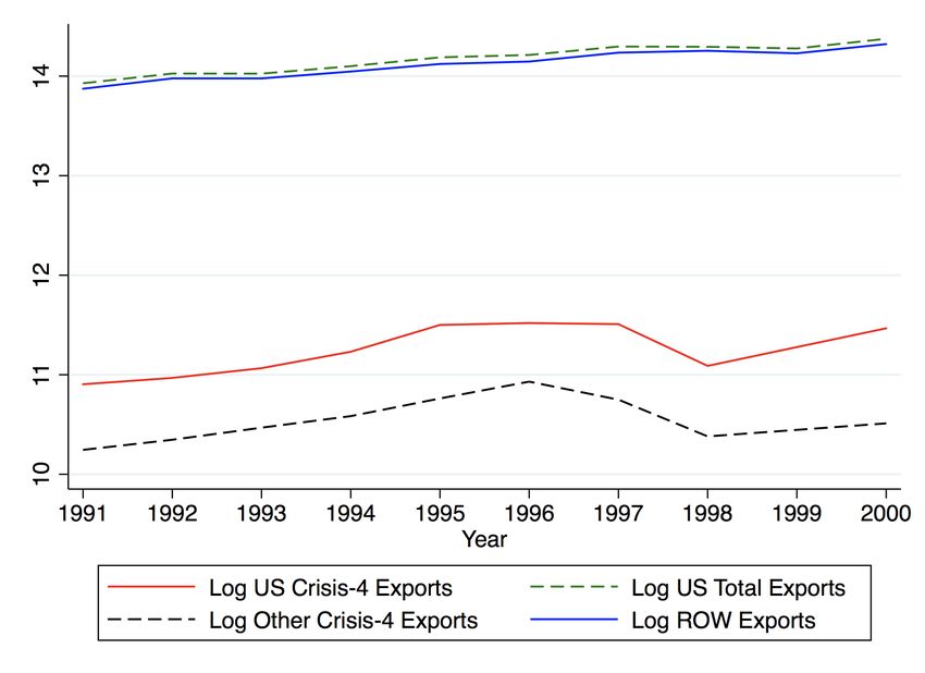
from the Roy (1951) structure used in Galle, Rodrı́guez-Clare, and Yi (2018). The advantage of this model

structure is it yields an estimation equation linking exports with local employment and wages. Furthermore,

I can use it to compute both partial and general equilibrium effects of the Asian Crisis shock. The Autor,

Dorn, and Hanson (2013) methodology captures only the partial effect.

   The general equilibrium gravity framework from Galle, Rodrı́guez-Clare, and Yi (2018), used to estimate

the effect of the China shock on income and welfare, assumes competitive labor markets with perfectly

inelastic labor supply and cannot capture effects of trade on employment. The specific-factors setting in this

paper, paired with the Roy model, does enable employment estimation. The Caliendo, Dvorkin, and Parro

(2019) dynamic framework computes general equilibrium employment effects of the China shock, but their

framework does not lend itself to measuring the effect of an export-transmitted shock such as the Asian Crisis

without making additional assumptions about the origin of the shock. Also, the theoretical framework in

this paper, coupled with the nature of the Asian Crisis identification, enables estimating a short-run degree

of worker heterogeneity (in tradable versus nontradable sectors) in response to a trade shock. This estimate

is on the lower end compared to the longer-run estimates found in existing literature (Adao, Arkolakis, and

Esposito (2017), Hsieh, Hurst, Jones, and Klenow (2019), Burstein, Morales, and Vogel (2019), and Galle,

Rodrı́guez-Clare, and Yi (2018)).

   Next, while there has been less work done on the effect of exports on labor market outcomes, McCaig

(2011) studies the effect of the US-Vietnam Bilateral Trade Agreement (BTA) on poverty and wages in

Vietnam, finding that increasing exports reduces poverty. McCaig and Pavcnik (2018) find that workers

reallocate from the informal to the formal sector in response to the positive export shock. Dauth, Findeisen,

and Suedekum (2014) study the effect of the rise in trade between Germany and the East over the period

1998-2008 on German labor market outcomes. Using a similar instrument to Autor, Dorn, and Hanson

(2013), the authors find significant employment increases as well as lower skilled worker turnover. In the US,

Feenstra, Ma, and Xu (2019) study the employment response to import competition from China and global

export expansion. They also use a similar methodology to Autor, Dorn, and Hanson (2013) and find that

Chinese import penetration reduces jobs, but export expansion creates jobs.

   This literature demonstrates there can be a substantial impact of a gradual export expansion on local

labor markets. The main contribution of this paper relative to earlier literature is that it demonstrates

that foreign crises can actually be transmitted to local labor markets via drops in export demand. More

generally, it quantifies a risk in engaging in exporting, which contrasts with the gains estimated by earlier

work. The identification strategy in this paper is also distinguished because the Asian Crisis was temporary,

unanticipated, arguably exogenous to US local labor markets, and can be used to estimate the dynamics

and duration of the impact. The permanent shocks exploited in existing literature do not lend themselves

                                                      3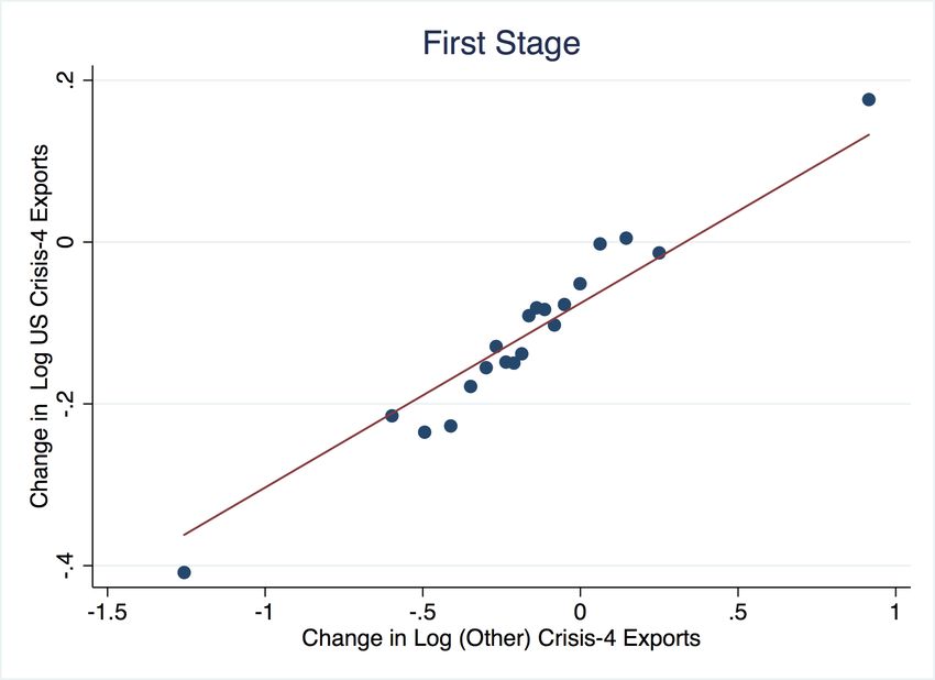
to estimating the hysteresis of a shock in the same way that can be captured by estimating effects of the

temporary Asian Crisis. The next section provides more details on the nature of the Asian Crisis shock.

3     The Asian Crisis of 1997

3.1     Background of the Crisis

    The Asian Crisis was marked in 1997 when Thailand devalued its currency relative to the dollar. Subse-

quently, gross domestic product (GDP) in Thailand, Indonesia, South Korea, and Malaysia plummeted by

12%, 16%, 8%, and 10%.3 These countries, known as the Crisis-4, entered deep recessions. Import demand in

those countries dropped as a result. Industries in the US, which had previously strong trading relationships

with those countries, saw large drops in exports. However, industries which did not have relationships with

those countries did not see changes in exports. Thus, the Asian Crisis is a natural experiment by which I

can identify the relationship between exports and employment.

    Pictured in Figure 1 are total US per-worker exports over the period 1991-2000 and per-worker exports to

Crisis-4 countries over the same period. I display the latter for both the US and for the five other countries

(on aggregate) that I use as my instrument. There is a slight decline in total US exports over the period

1997-1999 likely due to the sharp drop in exports to Crisis-4 countries in 1998.

                            Figure 1: Change in Total and Crisis-4 Exports, 1991-2000

Note: Natural log of total exports (green), natural log of US exports to Crisis-4 countries (red), and natural log of five other
countries’ exports to Crisis-4 countries (black) (Australia, Denmark, New Zealand, Spain, and Switzerland) over the period
1991-2000.
   3 Robert  Barro,    “Economic    Growth    in  East   Asia Before the   Crisis,”                NBER      Working     Paper,
http://unpan1.un.org/intradoc/groups/public/documents/APCITY/UNPAN014330.pdf

                                                               4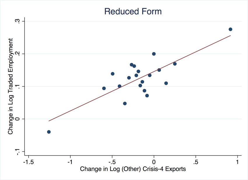
Exports to Crisis-4 countries dropped by 14.8 billion dollars between 1997 and 1998, a 30.9% decrease in

Crisis-4 exports and a 2% decrease in total exports given the share of Crisis-4 exports was approximately 7%

in 1997. Harrigan (2000) and Bernard, Jensen, Redding, and Schott (2009) find that US exports declined in

response to the Crisis. Both also find that exports to other countries in the world increased at the same time,

though at a much smaller rate. Specifically, Bernard, Jenson, Redding, and Schott (2009) pinpoint a 21%

decrease in exports to Crisis-4 countries with a corresponding 3% increase in exports to the rest-of-world

over the period 1996-1998. This suggests that the decline in US exports was exogenous and resulted from

the Crisis, not internal declines in output in the US. Additionally, Harrigan (2000) identifies industries which

were among the most affected, and the ones he lists include primary metals and transport equipment.4

    The calculated export declines as well as evidence from the literature on the Asian Crisis indicate that

this was a substantial shock to US export demand. Furthermore, as the Crisis was caused by a financial

crisis in East Asia, and US exports to other countries increased, the drop in demand for US tradable goods

was exogenous. In sum, the Asian Crisis of 1997 was a natural experiment which had heterogeneous and

significant effects across the US.

4     Theoretical Model for Employment and Wages

    I design a theoretical model as an extension of Kovak (2013). I do so in order to theoretically estimate

the effect of the Asian Crisis on local labor markets through the export channel, and measure heterogeneous

responses to the shock. Kovak (2013) constructs specific-factors model that predicts that when prices decrease

due to a tariff decline, wages will decrease. These changes are governed by the change in tariffs, the elasticity

of substitution between factors, and the cost share of the specific factor.

    I modify this model in two major ways. First, I conduct my analysis at the industry-CZ level. Second,

I embed a Roy (1951) model from Galle, Rodrı́guez-Clare, and Yi (2018) to determine labor supply. This

extension allows me to measure the degree of heterogeneity by sector in response to the Crisis. Furthermore,

these modifications yield a regression equation, and I can use the point estimates in my empirical section to

compute the shape parameter β (the degree of worker heterogeneity). This parameter helps demonstrate how

groups (in the context of the model, tradable and nontradable sectors) respond differentially to the Asian

Crisis shock. Accordingly, its estimate in a broader context will shed light on the potential for heterogeneous

responses to a possible trade shock. In the context of my data work, I am estimating a short run β, relative

to the long-run estimates in the literature.
   4 Bernard, Jensen, Redding, and Schott (2009) also document an increase in US imports from Asian countries during the

Asian Crisis, suggesting there may have been no significant supply chain or input-output linkage disruptions in the US at the
time.

                                                             5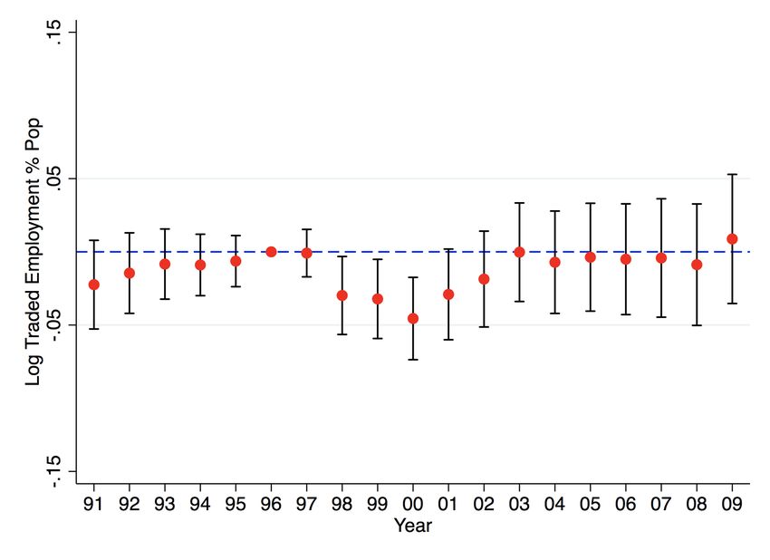
4.1      Setup

   The first few steps of this section follow Kovak (2013) closely, only departing to compute industry (j) -

CZ (i) specific terms. For the purposes of analysis, I consider two industries: tradable and nontradable. The

tradable sector may be hit with an export shock, whereas the nontradable sector cannot. I let Yij be output

in each industry-CZ, and aT ij and aLij be the quantities of specific factor and labor used in production.

Formally,

                                                  Tij = aT ij Yij                                            (1)

                                                  Lij = aLij Yij                                             (2)

Taking log differences of Equation 2 (x̂ = dlnx), letting hats denote proportional changes, noting the quantity

of the specific factor is fixed yields the following identities. As a result, in Equation 3 the change in output

is exactly equal to the inverse of the change in specific factor share. Equation 4 then links the change in

labor in a CZ-industry to the change in factor shares.

                                                   Ŷij = −âT ij                                            (3)

                                               L̂ij = âLij − âT ij                                         (4)

From Kovak (2013), the output price is equal to proportional shares of the labor wage and the specific factor

price.

                                            aLij wij + aT ij Rij = Pij                                       (5)

Log differencing Equation 5 , letting θj be the share of the specific factor in industry j, yields the expression

in Equation 6. Equation 7 follows from the definition of the elasticity of substitution between the specific

factor and labor.

                                           (1 − θj )ŵij + θj R̂ij = P̂ij                                    (6)

                                         âT ij − âLij = σij (ŵij − R̂ij )                                 (7)

Finally, rearranging and substituting 6 and 7 into 4 yields the industry-specific labor term in Equation 8

below.
                                                       σj
                                              L̂ij =      (P̂ij − ŵij )                                     (8)
                                                       θj

   Equation 8 is the change in labor in industry j in CZ i for a given change in exports. It indicates that

when there is a decline in export prices in the tradable industry, the corresponding employment decline

                                                          6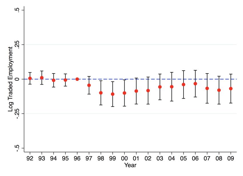
depends on the sizes of the wage decline, the elasticity of substitution between labor and the specific factor,

and the cost share of the specific factor. If there is no wage change, the employment change is relatively

larger.

4.2       Roy Model

   Departing from Kovak (2013), I allow labor to select into industries using a standard Roy model from

Galle, Rodrı́guez-Clare, and Yi (2018) (henceforth GRCY). In GRCY, there are Gg groups of workers from

country g, but for the purposes of analysis, I model only one country (the US). Each worker draws a

productivity zj in sector j drawn from a Frèchet distribution with shape parameter βi and scale parameters

Aij . As GRCY explain, the closer βi is to 1, the greater the degree of labor heterogeneity. Labor supply in

a commuting zone (Li ) is fixed, and worker allocation depends on workers selecting into industries (tradable

or nontradable).

   As in GRCY, the productivity draw z takes vector form with a value for each industry. z = (z1 , ....., zJ ).

Let Ωij = {z : wij zj ≥ wik zk ∀k} so that a worker in commuting zone i will choose to work in industry j

if z ∈ Ωij . Note that I allow for a commuting zone-industry specific wage rather than industry-specific in

GRCY. Finally, let Fi (z) be the probability distribution of z for workers in commuting zone i. Then the

share of employment in commuting zone i that works in industry j is given by

                                                                    Aij (wij )βi
                                                 Z
                                         πij =          dFi (z) =                                              (9)
                                                  Ωij                    Φi

where

                                                        X
                                                 Φi =        Aik (wik )βi
                                                         k

Log differencing (x̂ = dlnx), and noting the Aij are fixed,

                                                  π̂ij = βi wˆij − Φ̂i                                        (10)

I assume that labor supply in a CZ i is fixed, allowing me to equate L̂ij = π̂ij , This is a reasonable assumption,

because the Crisis was a short-term shock. I will later (in the Appendix) relax this assumption and allow for

flexible labor supply. Let Φ̂i to be a measure of the change in total labor market conditions in a commuting

zone. Consider a single elasticity βi = β. The solution is therefore given by Equations 11 and 12 below.

                                                             7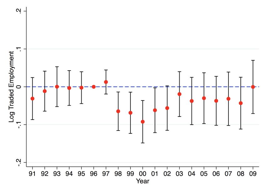
σ                  σj
                                                               β θjj                θj
                                                  L̂ij =             σj   P̂ij −         σj   Φ̂i                            (11)
                                                           β+        θj            β+    θj

                                                               σi
                                                               θij                   1
                                                  ŵij =          σij     P̂ij +       σ Φ̂i                                 (12)
                                                           β   + θij               β + θjj

    Thus, when there is a decrease in export prices in the tradable industry, employment and wages in

that industry decrease. The model predicts that employment in the other industry (nontradable) will thus

increase. There is a direct effect from exports, and an indirect general equilibrium effect from the shift in

CZ labor market conditions (Φ̂i ). As in Kovak (2013), the magnitudes of these changes depend on the cost

share of the specific factor and the elasticity of substitution between inputs. As an extension, I also allow

these changes to depend on the degree of worker heterogeneity β.

5     Estimation Design

5.1     Measuring Exposure to the Crisis

    Equation 11 informs the regression equation

                                           ∆LogLij = ηj ∆LogPij + ξj ∆LogΦi + ∆ij                                           (13)
                 σ               σj
                β θj             θj
                  j
where ηj =        σ     , ξ =      σ     , and ij is an industry-CZ error term. To estimate this expression, I follow
               β+ θ j           β+ θ j
                    j               j

Autor, Dorn, and Hanson (ADH 2013) and employ a stacked-difference (double-difference) strategy.

    Again following ADH, I first construct a measure of CZ exposure to the Crisis, CEP Wit . It is a measure

of a CZ’s per-worker exports to Crisis-4 countries based on its total employment and each of its compositional

industries’ employment.5 . It is constructed as follows:

                                                                          X Lijt−1 ∆Xjt
                                                 ∆CEP Wit =                                                                  (14)
                                                                          j
                                                                            LU jt−1 Lit−1

    In this equation, Lijt−1 is the start of period employment of each industry j of each CZ i. In my

subsequent estimation, I test a range of base years - 1991, 1992, and 1993. I note the US was in recession

in 1990-1991.6 In my preferred specification I use 1993 as a base year because it has the highest correlation
   5 Although other countries were affected by the Asian Crisis, I look only at Crisis-4 countries because these countries were

the most affected. Exposure to Crisis-4 exports therefore represents the best proxy to exposure to the drop in import demand
during the Crisis.
   6 If CZ’s were affected differently by the recession, it’s possible that the weighting in 1990-1991 would not accurately affect

CZ exposure to the Crisis during 1997-1999.

                                                                          8
with later years’ based measures while allowing for the greatest pre-period time difference. This is illustrated
by Figure 8 in the Appendix. LU jt−1 is each US (U) industry j’s start of period employment. The fraction
Lijt−1
LU jt−1 can be thought of as a CZ’s start of period share of each industry’s employment. Next, Xjt is each
Lijt−1 ∆Xjt
industry’s exports per year to Crisis-4 countries. The fraction LU jt−1 is a CZ i’s change in share of each
industry j’s Crisis-4 exports. Then, dividing by each CZ i’s start of period employment, Lit−1 , I obtain each
CZ’s share of each industry’s change in exports weighted by the number of workers in each CZ. I then sum
this figure across all industries to obtain CEP Wit , a measure of each CZ’s change in exports to Crisis-4
countries per worker per year.
Finally, I construct an analogous measure (∆CEP Woit ) using five developed countries’ exports to Crisis-4
countries (Australia, Denmark, New Zealand, Spain, and Switzerland). I use this to instrument for my main
independent variable. Changes in the five countries’ exports to Crisis-4 countries was a function of export
demand in Crisis-4 countries and unrelated to US labor market conditions. Furthermore, they are highly
correlated with US exports (both to Crisis-4 countries and in total) because they are both functions of export
demand in Crisis-4 countries. My instrument satisfies both exclusion (change in Crisis-4 exports in those
five countries are independent of US labor market conditions) and a strong first stage (Crisis-4 exports from
those countries are highly correlated with Crisis-4 exports from the US). It addresses a potential endogeneity
threat because import demand in the five other developed countries is independent of local labor markets in
the United States. Thus, I am identifying the change in employment and wages associated with a drop in
Crisis-4 export demand during the Crisis.
The calculation of these measures is similar to that of a Bartik (1991) instrument. In recent years, a
literature has blossomed that explores the implementation of these types of instruments. Three major papers
provide guidance on this topic: Adao, Kolesar, and Morales (AKM, 2019), Borusyak, Hull, and Jaravel (BHJ,
2020), and Goldsmith-Pinkham, Sorkin, and Swift (GPSS, 2021). The first paper provides a standard error
correction which accounts for potential share matrix correlation across observations. In the Appendix I
replicate my main estimation table using these “Bartik standard errors,” and find my estimates are robust
to this calculation.
BHJ provide “shock identification” conditions through which a shift-share IV is valid, and provide evi-
dence that the estimation in Autor, Dorn, and Hanson (ADH, 2013) is robust. The two identifying assump-
tions from BHJ are 1) the shocks are uncorrelated with the error term and 2) the shocks are independent
across observations. As argued in the earlier paragraph, the variation from the Crisis demand from non-US
countries is exogenous to local employment in the US, satisfying (1). On the second, each commuting zone
is composed of different ranges of industries which receive different amounts of the Crisis shock, suggesting
the shocks are independent across observations and satisfying (2).
9Finally, GPSS demonstrate that a Bartik SSIV is equivalent to GMM with industry shares as instruments.
However, if the shares are endogenous then the Bartik estimator may not be a valid IV. I argue that because
the Asian Crisis was an unexpected and temporary shock the potential for correlated “unobserved shocks”
causing endogeneity of the share identification is not as potent in this case. In sum, the identification in this
paper is informed by this novel Bartik literature.
As stated earlier, in my main regressions I employ a logged stacked-difference empirical strategy. I choose
this double-difference specification because it allows me to compare the effect of the drop in Crisis-4 exports
from 1996-1998 to the size of the change in exports in the pre period, 1993-1996. In my baseline estimation
of the effect of exports on traded employment, I use CZ-wide start-of-period demographic controls and CZ
and time fixed effects to balance the sample. In my main regressions, I measure CEP Wit and CEP Woit
using 1993 as a base year and estimate stacked differences from 1993-1996 and 1996-1998. I choose 1993 as a
base year because, as shown in Figure 6 in the Appendix, the 1993 based measure has the highest correlation
with later years’ (closer to the Crisis) measures while allowing for the longest pre-period time difference.
The final estimation equation is:
∆LogLijt = ηj ∆LogCEP Wit + ξj ∆Dit + φi + φt + ∆it (15)
where Dit are the start-of-period demographic controls and φ are CZ and time fixed effects. Note I
use only two time periods, so two observations per CZ: 1993-1996 and 1996-1998. LogLijt is the log of
employment in each sector (traded and nontraded).
I cannot directly estimate Equation 11 because I do not have data on Φi , the CZ-wide general equilibrium
term. I also do not have data on export prices, so I use export values (price × quantity). Furthermore, I
am using change in Crisis-4 exports on the right hand side rather than change in total exports as my model
specifies.
Also, while interpretation of my model is the percent effect of a one percent change in Pijt on Lijt ,
the interpretation of this difference is the log-point effect of a one log-point decline in Crisis-4 exports on
industry employment. For small percent changes in X, dlnX = logX 0 − logX, but the percent change in
Crisis-4 exports in my sample is sufficiently large that the identity does not hold. Note that it does hold
for total exports in my sample and I will exploit this in my structural estimation. Also, running a simple
log change specification of employment on Crisis-4 exports yields a lower coefficient than the double-log-
difference, but the simple log change of employment on total exports yields the same coefficient. Across all
empirical specifications I prefer the double-log-difference to the simple log change because it allows me to
exploit a comparison between the Crisis period to the pre-period, following Autor, Dorn, and Hanson (2013),
10for robustness.
To further address these issues in subsequent structural estimation of the β parameter I will difference
traded and nontraded sectors, use total exports, and convert prices to quantities using the ratio of import
price drop to value drop in Crisis-4 imports from Higgins and Klitgaard (2000).
Next, using CEP Wit , I am able to measure how important Crisis-4 exporting industries were to a CZ’s
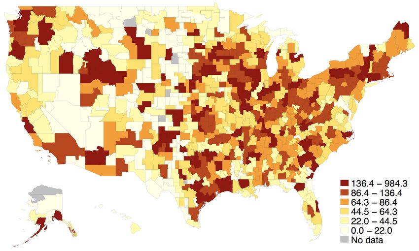
employment before the Crisis. Figure 2 displays this wide geographic variation.7
Figure 2: CZ Exposure to Crisis-4 Exports
Note: Level of per-worker exports to Crisis-4 countries in 1992 plotted over a map of the US. Darker colors indicate higher
levels of exposure.
5.2 Data
5.2.1 Sources
Next, to estimate the effect of the Asian Crisis of 1997 on employment and wages, I obtain data from a
range of sources. I pull data from Comtrade on the US’s, Australia’s, Denmark’s, New Zealand’s, Spain’s,
and Switzerland’s exports to Crisis-4 countries. This data is at the HS-6 level, and I use David Dorn’s
crosswalks to convert it to the SIC-87 level and then aggregate to the CZ level.
I use County Business Patterns (CBP) employment data and Quarterly Census of Employment and Wages
(QCEW) wage data. I note that a shortcoming of these datasets are that the raw datasets do not include
6-digit NAICS codes for all industries and counties. This occurs because in counties where one company
is an entire industry, including employment and wage information would clearly reveal private information
about that county. To solve this issue, I use CBP data imputed by Fabian Eckert, who runs an imputation
algorithm to fill in missing data. The data is in SIC-87 format until 1997 and then switches to NAICS-6
7 As discussed in Section 5.2.2, during cleaning I drop 9 CZ’s from my sample which have missing trade data so they are
missing in this plot. The 7 CZ’s with missing population data are included because they do have trade information.
11starting in 1998, so I use a crosswalk from Dorn to convert the data from NAICS-6 to SIC-87.8 Second, I use
aggregate industry wage data from the QCEW. The survey is a Bureau of Labor Statistics (BLS) publication
which contains “a quarterly count of employment and wages reported by employers covering 98 percent of
US jobs, available at the county, MSA, state and national levels by industry.”9
Next, I obtain data from Schott (2008) which contains trade data by 6-digit NAICS industry and country.
It provides import and export numbers for 463 6-digit industries, agricultural (NAICS 1) and manufacturing
(NAICS 3), and 241 countries for the years 1990-2009. It also includes data on exports to Crisis-4 countries.
This data comes from the Census, and is comprehensive. I use this total export data for Figure 1 and to
provide one measurement of β, the (short-run) degree of worker heterogeneity in my model. I also consider
this dataset to contain all traded industries, and accordingly use this designation to distinguish traded
employment from nontraded employment.10
I obtain data from the US 1990 Census for county-level education numbers. I use this to generate
geographic-level education numbers to split my sample and perform analysis regarding high and low education
CZs. This data contains 1990 education numbers for 3,141 counties. Using this data, I classify a highly
educated worker as someone who has at least a Bachelor’s degree. I use population numbers from this
dataset as a base group from which I calculate percent of high and low educated workers.
Next, I obtain data on unemployment by county from Local Area Unemployment (LAU) data from the
Bureau of Labor Statistics. I obtain population data from the Surveillance, Epidemiology, and End Results
Program (SEER). I aggregate these from the county level to the CZ level. Paired with the employment data,
I am able to therefore study a complete picture of what happens to a CZ’s inhabitants after an export shock.
Finally, in order to convert my data from county to CZ, I use conversion data from Autor, Dorn, and
Hanson (2013). I thus have a dataset at the CZ-industry-year level, covering 741 CZs and it contains
comprehensive labor market measures. I use years 1993-1998 for my main regressions, and extend to 2009
to explore persistence of the shock.
8 In the crosswalk, Dorn provides a weight variable which is the percent of the national NAICS 1997 code corresponds to
each SIC-87 code. To convert the data from the former to the latter, I multiply employment by this weight variable and then
sum across NAICS codes within each SIC code. One problem with this is that in some CZs, only one SIC corresponding to
a specific NAICS code is present, so this method may under-count employment for some observations. However, this issue is
dispersed across the full sample and is independent of the Crisis-4 export variation. Also, I estimate that in approximately 5%
of SIC-CZ pairs, imputed 1998 employment is less than 50% of 1997 employment. Of this 5%, the mean difference in imputed
1997 and 1998 employment is 80 workers. I note that these statistics also include true drops in employment. For additional
robustness, in Appendix Table 8 I replicate my preferred specifications from Table 2 after constructing SIC-CZ employment
without using the Dorn-NAICS weights (which over- rather than under-counts employment). The results are unchanged and
the point estimates are close. Finally, in Section 6.3’s event study estimation, I find that traded employment fully recovered
4-5 years after the Crisis. If the weighting change were driving variation, the post-1997 drop would appear permanent.
9 Bureau of Labor Statistics, Quarterly Census of Employment and Wages, October 4, 2016
10 For the QCEW aggregate industry wage data, I approximate and designate NAICS 1-digit codes 1, 2, and 3 as tradable
because most tradable industries (by the definition used in the rest of the paper) fall into these sectors.
125.2.2 Summary Statistics
Table 1 contains means for my full sample. The average percentage in 1990, the latest Census year prior
to the start of the sample, of workers with a Bachelor’s degree in a CZ is approximately 14%, suggesting
that most CZs were more heavily populated with less-educated workers in 1990. This number ranges up to
39% in my data. There are 741 CZs in the US. I drop 9 CZs which had no trade in 1991 to balance the
comparison. In my estimation, there are an additional 7 CZs which I could not match population data for,
so they are dropped from analysis. This brings my regression sample to 725 CZs.11 In the Appendix Table
9, I replicate Table 1 using population-weighted means.
Table 1: Summary Statistics
ExportsP Wit 2103.6
CrisisExportsP Wit 115.0
CrisisExportsP Woit 58.52
Unemployment Rate 6.148
Population 361790.9
% Educated 0.140
Employment (Annual) 294724.1
Traded Employment 21684.0
Non Traded Employment 273040.1
Wage (Average Weekly) 429.5
Traded Wage (Average Weekly) 515.7
Non Traded Wage (Average Weekly) 406.4
N 5825
Note: Commuting zone means reported over main regression sample period (1993-1998). 725 CZs in regression
sample.
6 Empirical Results
6.1 Full Sample Results
In this section, I employ a range of estimation techniques to measure the effect of the drop in US exports
during the Asian Crisis on local traded employment, described in Section 5. Table 2 contains the results
from these specifications. Column 1 uses 1993 employment weights as discussed in Section 5.1. The rest of
the columns in Table 2 contain robustness on this estimate. I employ a range of strategies: re-computing
CEP Wit and CEP Woit while calculating a 1996 weighting base for the second period difference, exploiting
1992 as a base year, using log of traded employment share of population as the outcome, measuring differences
11 The sample is slightly unbalanced, but in the estimation years (1993,1996,1998) the common denominator is 725 CZs.
13starting in 1991 and 1992 instead of 1993, or using total per-worker exports as the explanatory variable. The
results in Table 2 show the estimates are robust to each of these strategies and the coefficients are similar.
Table 2: Traded Employment Response to Asian Crisis
(1) (2) (3) (4) (5) (6) (7) (8)
∆LogCEP Wit 0.356∗∗∗ 0.356∗∗∗ 0.136∗∗∗ 0.530∗∗∗ 0.191∗∗∗ 0.282∗∗∗ 0.235∗∗ 0.211∗∗
(0.108) (0.103) (0.0415) (0.125) (0.0511) (0.0933) (0.0955) (0.0910)
Controls Y Y Y Y Y Y Y Y
CZ FE Y Y Y Y Y Y Y Y
Year FE Y Y Y Y Y Y Y Y
N 1450 1450 1450 1450 1450 1450 1450 1450
First Stage F-Stat 22.61 12.89 22.61 17.52 17.52 19.51 26.09 30.46
AKM (2019) Bartik SE (0.0760) (0.0725) (0.0293) (0.104) (0.0457) (0.0658) (0.0674) (0.0641)
∗
p < 0.10, ∗∗ p < 0.05, ∗∗∗ p < 0.01
Note: Stacked difference regressions estimating Equation 15 using the log of traded employment on log of LogCEP Wit . All regres-
sions are estimated in changes and ∆LogCEP Wit is instrumented using ∆LogCEP Woit . Column 1 (preferred specification) bases
LogCEP Wit in 1993 and estimates stacked differences over the periods 1996-1993 and 1998-1996. Column 2 replaces LogCEP Wit with
LogEP Wit (total per-worker exports). Column 3 uses log traded employment share of working age population as the outcome. Columns
4 and 5 re-calculate LogCEP Wit using a 1996 base for the second period difference, with Column 4 using log traded employment and
Column 5 using log traded employment share of population as the outcome. Column 6 bases LogCEP Wit in 1992. Finally, Columns 7
and 8 base LogCEP Wit and begin the first period difference in 1992 and 1991 respectively. All specifications use demographic controls
(young share of population, nonwhite share of population, and female share of population) and a control for population. Adao, Kolesar,
and Morales (2019) Bartik standard errors alternatively reported, using 1993 industry-CZ share weights.
In subsequent empirical specifications, I employ the 1993 pre-period weighting, 1996 Crisis-period reweight-
ing specification from Column 4. I choose this specification for the empirical estimates because it is consistent
with earlier literature such as Autor, Dorn, and Hanson (2013) for this topic and allows for closer correlation
between the Crisis period difference and its weights. I note that the estimates using the simple 1993 weight
are similar.
Table 2 also reports Bartik standard errors, following Adao, Kolesar, and Morales (2019). These standard
errors correct for potential residual correlation due to similar industry structures.12 These Bartik standard
errors I estimate are similar and modestly smaller than those calculated by clustering, which can occur
depending on the data’s sector-CZ makeup.
Next, using the specification from Column 4 as my preferred specification, below in Figure 3 is a plot of the
first stage of ∆LogCEP Wit on ∆LogCEP Woit (left) and the reduced form of ∆LogLijt on ∆LogCEP Woit
(right). I find that Crisis-4 exports from other related countries is highly correlated with US Crisis-4 exports.
Furthermore, the reduced form plot on the right also shows a strong relationship between change in traded
employment and the Crisis shock.
12 The AKM code used to compute them requires including a industry-region employment share matrix. Because the preferred
weight year is 1993, I construct this matrix using 1993 data.
14Figure 3: CZ Exposure to Crisis-4 Exports
Note: First stage (left) and reduced form (right) of the instrumental variables specification of ∆LogT radedEmpit on
∆LogCEP Wit . Binscatter groups the data points and plots the mean for each bin. The solid line represents the regres-
sion estimator.
In this section I also explore persistence of the effect of the Crisis on employment, heterogeneity across
highly and relatively less educated CZs, and other labor market effects. In these alternate empirical spec-
ifications, I employ the 1993 pre-period weighting, 1996 Crisis-period reweighting specification described
above. I choose this specification for the empirical estimates because it is consistent with earlier literature
such as Autor, Dorn, and Hanson (2013) for this topic and allows for closer correlation between the Crisis
period difference and its weights. I note that the estimates using the simple 1993 weight are similar.
I next measure the effect of the export drop on a range of labor market outcomes: nontraded employment,
traded and nontraded wage, total employment, the unemployment rate, labor force size, and population.
Table 7 in the Appendix contains these estimates. I find modest effects on nontraded and aggregate em-
ployment, but no other labor market indicators, possibly because of the small and temporary nature of the
shock.
Next, I split my sample into quintiles of 1993 values of CEP Wit and estimate a binned specification,
testing whether higher ex-ante exposure to Crisis-4 exports led to a greater drop in employment during the
Crisis. Table 3 contains these results. I report both OLS (Columns 1 and 3) and the reduced form (Columns
2 and 4) because the instrument is weak with disaggregation.13 The coefficients are approximately increasing
in magnitude by bin number, where Bin 5 is the highest exposed. As an alternate specification in Columns
5 and 6, I split my sample into two bins based on median values of 1993 CEP Wit and employ a difference-
in-difference technique. I again find that the highly exposed CZs had greater declines in traded employment
during the Asian Crisis. For the simple difference-in-difference with two bins the instrument has more power
so I am able to employ IV.
13 In later event-study specifications when estimating shock persistence I only report the reduced form to address potential
endogeneity concerns with OLS. Namely, that ex ante US export exposure could be simultaneous with subsequent employment
fluctuations due to traded-sector trends.
15Table 3: Traded Employment Response to Asian Crisis, Binned Specifications
(1) (2) (3) (4) (5) (6)
Crisis-4 Exposure Bin 2 -0.195∗∗∗ -0.156∗∗∗ -0.0572∗∗ -0.0372
(0.0556) (0.0550) (0.0266) (0.0264)
Crisis-4 Exposure Bin 3 -0.226∗∗∗ -0.249∗∗∗ -0.0844∗∗∗ -0.0981∗∗∗
(0.0545) (0.0545) (0.0255) (0.0259)
Crisis-4 Exposure Bin 4 -0.228∗∗∗ -0.222∗∗∗ -0.0789∗∗∗ -0.0789∗∗∗
(0.0545) (0.0539) (0.0257) (0.0256)
Crisis-4 Exposure Bin 5 -0.246∗∗∗ -0.226∗∗∗ -0.0949∗∗∗ -0.0850∗∗∗
(0.0551) (0.0548) (0.0265) (0.0264)
Crisis-4 High Exposure -0.244∗∗∗ -0.112∗∗∗
(0.0469) (0.0253)
Controls Y Y Y Y Y Y
CZ FE Y Y Y Y Y Y
Year FE Y Y Y Y Y Y
N 5075 5075 5075 5075 5075 5075
First Stage F-Stat 269.7 269.7
∗
p < 0.10, ∗∗ p < 0.05, ∗∗∗ p < 0.01
Note: Binned specifications estimating the effect of the fall in US exports to Crisis-4 countries on local traded employment. Columns
1-4 employ 5 CZ bins of 1993 Crisis-4 per-worker exports and Columns 5 and 6 employ 2. Columns 1, 3, and 5 use log of traded
employment as the outcome and Columns 2, 4, and 6 use log of traded employment share of working age population. Finally, Columns
1 and 3 report OLS and Columns 2 and 4 report the reduced-form because the instrument is weak for the disaggregated bins, and
Columns 5 and 6 report IV. All specifications use demographic controls (young share of population, nonwhite share of population, and
female share of population) and a control for population.
6.2 Heterogeneity in High and Low Education CZs
Next, I estimate heterogeneous effects on CZs that differ in composition of worker education. I divide
the sample into terciles of 1990 CZ education (percent with at least a Bachelor’s degree).14 I then run the
specification in Equation 15 on the split sample. Table 4 contains the estimates from these specification.
I find that all of the labor market adjustment occurred in relatively low-education CZs: both traded and
nontraded employment in low-education CZs fell significantly. According to the model in Section 4, the
latter effect could be driven by changes in the the general-equilibrium Φ term.
14 I employ terciles rather than quartiles because the instrument loses power with further disaggregation.
16Table 4: Heterogeneous Response to Asian Crisis Shock by Education Shares
Traded Emp Nontraded Emp Traded Wage Nontraded Wage Total Emp Unemployment Labor Force Population Working Age
(1) (2) (3) (4) (5) (6) (7) (8) (9)
Education Bin 1 0.501∗∗∗ 0.200∗∗∗ -0.0136 -0.00821 0.0709∗∗∗ -0.0189 0.00972 0.0105 0.00622
(0.126) (0.0320) (0.0249) (0.0184) (0.0195) (0.0484) (0.0110) (0.0118) (0.0121)
Education Bin 2 0.530∗∗∗ 0.0849∗∗∗ 0.00740 0.0115 0.0460∗∗ -0.0342 0.00242 0.00803 0.00493
(0.119) (0.0315) (0.0213) (0.0186) (0.0204) (0.0513) (0.0106) (0.0116) (0.0120)
Education Bin 3 0.541∗∗∗ 0.0421 -0.00413 -0.00137 0.0377∗ -0.0301 -0.00898 0.0190 0.0128
(0.134) (0.0295) (0.0221) (0.0182) (0.0207) (0.0480) (0.0104) (0.0186) (0.0185)
Controls Y Y Y Y Y Y Y N N
CZ FE Y Y Y Y Y Y Y Y Y
Year FE Y Y Y Y Y Y Y Y Y
N 1450 1450 1418 1450 1450 1450 1450 1450 1450
First Stage F-Stat 5.889 5.889 4.876 5.889 5.889 5.889 5.889 6.022 6.022
∗
p < 0.10, ∗∗ p < 0.05, ∗∗∗ p < 0.01
Note: Stacked difference regressions estimating Equation 15 using the log of traded employment on log of CEP Wit . All regressions
are estimated in stacked differences over the periods 1993-1996 and 1996-1998. ∆LogCEP Wit is instrumented using ∆LogCEP Woit .
Outcomes are logs of traded employment, nontraded employment, traded wage, nontraded wage, total employment, unemployment rate,
labor force, population, and working age population. Split into 3 bins of 1990 CZ share with a Bachelor’s degree. All specifications
use demographic controls (young share of population, nonwhite share of population, and female share of population) and a control for
population.
6.3 Persistence
Finally, I test if the effects of the Crisis on traded employment lasted past the Crisis years. I use
the reduced form of the stacked difference specification from Column 4 of Table 2, base my sample with
1991 Crisis-4 exports so as to extend the time panel, and construct differences from 1996 value of traded
employment for each year from 1992-2009.15 I compare this against the change in Crisis-4 exports from
1996-1998. An advantage of this specification is I can both test for pre trends (did the drop in Crisis-4
exports affect traded employment prior to Crisis years?) and explore persistence of the Crisis past 1998 (did
the drop in exports have a permanent effect on employment, or did it adjust back to pre-1998 levels?).
15 The instrument is weak with yearly disaggregation, and reporting OLS for this figure would raise the same concern as in
Table 2, that change in employment is simultaneous with change in exports.
17Figure 4: Time Dynamics of Crisis Effects
Note: Figure 4 contains a stacked difference specification, where the explanatory variable is the difference in Crisis-4 exports
from 1996-1998 stacked with the difference from 1991-1996. The dependent variable is stacked cross-sectional differences of log
of traded employment using 1996 as the comparison year. The 1991-1996 coefficient is omitted in order to generate the stacked
difference and 1996, the base difference year, is normalized to zero. Sample from 1991-2009.
I find a sharp drop in traded employment associated with the fall in exports during the Crisis, and effects
persisted through at least 2000, three years past the start of the Crisis. Coefficients in the rest of the sample
are measured slightly imprecisely, but I find that there was gradual adjustment to the norm so that the
coefficient point estimate returns to approximately zero by 2005-2006. A concern with these estimates is
that perhaps the Crisis shock was not transitory, that exports to Crisis-4 countries fell permanently during
the Crisis and did not recover until at least when I observe employment recovery in Figure 4. Below is a
plot of log Crisis-4 exports and log total exports aggregated from the industry level from 1990-2010. Note
that this is different from Figure 1, which plots per-worker exports.
I find that exports to Crisis-4 countries returned to trend in 2000. This result in itself, when paired with
Figure 4, suggests there was some element of sluggish adjustment: in Figure 4, employment remains below
trend in 2000. In Figure 5, both total and Crisis-4 exports fell again in 2001, likely due to the US recession.
They return to trend in 2004. In Figure 4, the point estimate remains below trend but the confidence interval
widens to include zero.
18Figure 5: Time Dynamics of Crisis Effects
Note: Figure 5 contains of Crisis-4 exports (red) and log of total exports (black dash) plotted from 1990-2010.
Therefore, a concern with the estimates from Figure 4 is that the post-2000 sluggish adjustment could
be picking up the effect of the drop in exports during later years when estimating the effect of the drop
in exports from 1996-1998. To address this concern, I interact bins for high exposure to the Crisis shock
based on 1990 CZ per-worker Crisis-4 exports with yearly indicators. An advantage of this specification is
I can directly compare the time trends of more versus less exposed CZs to the Crisis. This specification is
not explicitly testing the effect of the export drop during the Crisis; rather, it is exploiting heterogeneity in
ex ante exposure to the Crisis. Accordingly it is likely more robust to confounding effects from later years’
export declines than the specification from Figure 4.
A concern with simply splitting by start-of-sample Crisis-4 exports is that a high value of Crisis-4 exports
is correlated with a high amount of trade, so those estimates would also capture the 2001-2003 fall in US total
trade and overestimate persistence. Accordingly, for the event study estimates in Figure 6, I split my sample
based on 1990 Crisis-4 exports divided by total US 1990 exports. I employ the reduced form of Crisis-4
exports (from other developed countries) to address potential endogeneity concerns. The “treatment” group
for this exercise will therefore be the CZs containing industries for which trade with Crisis-4 countries was
relatively important while controlling for the total amount of trade the CZ was engaged in. This design is
therefore able to capture the time dynamics of the Crisis while also being robust to potential confounding
trends affecting US trade. I run this specification for both log of traded employment and log of traded
employment share of population. I plot the coefficient estimates in Figure 6 below.
19Figure 6: Time Dynamics of Crisis Effects
Note: Figure 6 contains two event study specifications, where the explanatory variables are bins of exposure to the Crisis
shock based on 1990 CEP Woit weighted by total US exports, interacted with period indicators. The dependent variable in the
left plot is log of traded employment, and the dependent variable in the plot on the right is log of traded employment share
of population. Controls are included for log of population, youth share of population, female share of population, nonwhite
share of population, and log of working-age population. Commuting zone fixed effects also included, and standard errors are
clustered at commuting zone level. Sample from 1991-2009.
In both plots of Figure 6, there is no evidence of pre-trends, and in 1998 traded employment in the
treatment CZs discontinuously drops relative to trend. The difference lasts for a couple years but is not
permanent: the coefficients return to zero by 2003. Thus the result from Figure 6 is consistent with that
of Figure 4, but provides additional robustness in that it also controls for trends to total exports. In sum,
the evidence from Figures 4-6 suggest that there was some sluggish US employment adjustment back to the
norm after the Crisis shock was transmitted locally via the export channel.16
7 Model Implied Estimates
7.1 Measuring β, the [Short Run] Degree of Worker Heterogeneity
Next, I use the theoretical model from Section 4 to measure β, the degree of worker heterogeneity. In
my data, it is a short-run elasticity, rather than the estimates from earlier work which measure longer-run
elasticities. From the Frèchet distribution we know β > 1. When β → 1 the general equilibrium term Φ̂ → 0,
so effects of the export shock are concentrated in the traded industry only. Thus, when β → 1 there are
greater distributional consequences of exporting. Estimating the value of β is therefore important when
predicting the CZ-wide effects of an export shock.
To estimate β, I calibrate Equation 11 from my model. As discussed earlier, I do not have a good
16 To generate this persistence using the model from Section 4, I can extend the model to three periods, where the first
difference reflects the negative shock, the second is a return to normalcy, and the third reflects no change (normal times). Firms
cannot make negative profits, so in the face of the negative demand shock in the first period they perfectly adjust employment
downward. There is an adjustment cost following the downward shock because firms cannot immediately re-hire labor, so that
in the second period the pricing identity given by Equation 5 is a function of period 2 prices and employment remains low.
By the third period, the adjustment has occurred and employment returns to pre-shock levels. This generates the sluggish
adjustment result found in this section.
20measurement of Φit . However, what I can do is difference Equation 11 between traded and nontraded
employment as nontraded Crisis-4 exports are zero. This method eliminates the Φ term. Thus I estimate
σ
β θjj
L̂itr − L̂int = σj P̂ij
β+ θj
I then run the following specification:
∆LogT radedEmploymentit − ∆LogN ontradedEmploymentit = η∆logCEP Wit + φt + φi + it (16)
where φi and φt are CZ and time fixed effects and it is a CZ-time error term. For precision, I note again
that Pij is a price and CEP Wit is a quantity, so I construct a quantity-to-price conversion using the ratio
of import price drop to value drop in East Asian imports from Higgins and Klitgaard (2000). I find that
P̂it = µ∆LogCEP Wit where µ = 0.45. Thus the above expression can be written as
η
∆LogT radedEmploymentit − ∆LogN ontradedEmploymentit = P̂it + φt + φi + it (17)
µ
I thus solve
β σθ η
σ = (18)
β+ θ µ
I test using both Crisis-4 exports and total exports as my explanatory variables, but use the results from
the latter specification as it my model estimates the effect of total exports. Furthermore, as explained earlier
the percent change in total exports in my sample is small, so dlnX = lnX 0 − lnX and the double-differencing
specification captures the effect of X̂ijt . I also test adding the demographic controls from the earlier tables.
This structural estimation employs the 1993 weighting (for both periods) method rather than reweighting
in 1996 because it is most consistent with the interpretation of the model in Section 4.17
I then calibrate my model with a range of values for θ and σ. My baseline calibration uses σ = 0.65, the
midpoint of the estimate range of the elasticity of substitution between labor and capital from Knoblach,
Roessler, and Zwerschke (2020). In an alternate measurement I employ σ = 0.5, which is their measurement
of the short-run elasticity of substitution. Next, Kovak (2013) measures θ, the specific factor share, as one
17 A concern with reweighting for the structural estimation is that the model is designed as a single difference (as discussed
earlier, the double-difference estimation strategy is employed in this paper for the purpose of identification). Accordingly, for
the structural work reweighting in 1996 would alter the regression coefficient point estimate to capture industry makeup shifts
over 1993-1996. It would distort away from the true β because the model assumes the weights are constant in the pre-period.
Employing 1993 weights across both periods enables a more direct comparison between the pre-period and the Crisis period,
more closely follows the model, and allows for a more accurate measurement of β.
21You can also read