Fitting ODE models of tear film breakup
←
→
Page content transcription
If your browser does not render page correctly, please read the page content below
Fitting ODE models of tear film breakup
                                               Tobin A. Driscoll1 , Richard J. Braun1 , Rayanne A. Luke2 , Dominick Sinopoli1 , Aashish
                                                    Phatak1 , Julianna Dorsch1 , Carolyn G. Begley3 , and Deborah Awisi-Gyau4
arXiv:2210.03593v2 [math.NA] 21 Feb 2023

                                                     1
                                                      Department of Mathematical Sciences, University of Delaware, Newark, DE 19716, USA
                                           2
                                               Department of Applied Mathematics and Statistics, The Johns Hopkins University, Baltimore, MD 21218
                                                                                              USA
                                                             3
                                                               School of Optometry, Indiana University, Bloomington, IN 47405, USA
                                                             4
                                                               Alcon Research LLC, 6201 South Freeway, Fort Worth, TX 76134, USA

                                                                                                Abstract
                                                       Purpose. Several elements are developed to quantitatively determine the contribution of
                                                   different physical and chemical effects to tear breakup (TBU) in subjects with no self-reported
                                                   history of dry eye or other ocular surface disease. Fluorescence (FL) imaging is employed to
                                                   visualize the tear film and to determine tear film (TF) thinning and potential TBU.
                                                       Methods. An automated system using a convolutional neural network is deployed that was
                                                   trained and tested on more than 50,000 images from FL imaging experiments. The trained
                                                   system could identify multiple TBU instances in each trial. Once identified, extracted FL
                                                   intensity data was fit by mathematical models that included tangential flow along the eye,
                                                   evaporation, osmosis and FL intensity of emission from the tear film. The mathematical models
                                                   consisted of systems of ordinary differential equations for the aqueous layer thickness, osmolarity,
                                                   and the FL concentration; they are a local approximation to TF thinning and/or TBU dynamics.
                                                   FL intensity was computed using the resulting thickness and FL concentration. Optimizing the
                                                   fit of the models to the FL intensity data determined the mechanism(s) driving each instance
                                                   of TBU and produced an estimate of the osmolarity within TBU.
                                                       Results. Initial estimates for FL concentration and initial TF thickness agree well with prior
                                                   results. Fits were produced for N = 467 instances of potential TBU from 15 non-DED subjects.
                                                   The results showed a distribution of causes of TBU in these healthy subjects, as reflected by
                                                   estimated flow and evaporation rates, which appear to agree well with previously published
                                                   data. Final osmolarity depended strongly on the TBU mechanism, generally increasing with
                                                   evaporation rate but complicated by the dependence on flow.
                                                       Conclusion. The method has the potential to classify TBU instances based on the mechanism
                                                   and dynamics and to estimate the final osmolarity at the TBU locus. The results suggest that
                                                   it might be possible to classify individual subjects and provide a baseline for comparison and
                                                   potential classification of dry eye disease subjects.

                                           1      Introduction
                                           In this paper, we generate quantitative estimates of important parameters for the tear film on the
                                           surface of the eye in healthy subjects. We do this with what we believe, at the time of writing, to

                                                                                                    1
Fitting ODE models of TBU 2
be unprecedented precision and quantity. The dataset creates a preliminary baseline for a small
population of subjects without dry eye disease (DED). The importance of this baseline is that it may
be used to contrast what is found for a population with DED, thus leading to better understanding
of the mechanisms at work in this disease that affects millions of people [86, 87, 95, 96]. Though this
work does not give a complete baseline for non-DED eyes, or a contrast with data for DED eyes,
we develop the method in detail and explain how it can reveal the mechanisms behind individual
instances of thinning and tear breakup (TBU) in the tear film (TF).
The introduction is structured as follows. Firstly, we give some background on the tear film,
ocular surface and DED. Secondly, we briefly discuss some related methods for imaging the tear
film. Thirdly, we discuss methods to extract data about tear film dynamics. Finally, we discuss
mathematical models for tear film dynamics, and best fits of those models to data extracted from
the tear film.
Tear Film The TF plays an important role in vision and ocular surface health [75]. The TF
is established during a blink, and lubricates the cornea and the conjunctival surfaces lining the
gap between the lids and the globe [83]. The air/tear film interface causes the tear film to have
the most powerful refractive surface in the eye; thus, keeping that surface smooth and regular is
essential to clear vision [99]. When the TF fails to uniformly coat the ocular surface, it is said that
tear breakup has occurred [24, 78]. TBU may cause the ocular surface to be exposed to cooling [8,
36, 66] and evaporation [35, 76], and evaporation may lead to tear hyperosmolarity [15, 27, 53, 58]
and mechanical stimulus to the surface [3]. The exposure of the ocular surface to hyperosmolarity
from TBU is thought to play a central role in the etiology of DED [27, 53] which affects millions
of people [95]. As a result of this significance, TBU dynamics have been studied for more than 50
years using a variety of methods [78, 107]. Clinically, the instability of the tear film is measured
by the technique of tear breakup time (TBUT), in which the time to the first break or irregularity
of the tear film is measured.
Imaging methods The imaging methods for TBU dynamics are numerous. Here we list a few of
them: visualization with dyes such as fluorescein (FL) [23, 78]; reflection of a pattern using a grid
[69] or placido disc images [59]; interferometry and spectrometry [29, 33, 40, 51, 88]; simultaneous
imaging with fluorescence (FL) imaging and retroillumination [15]; and simultaneous FL imaging
with interferometry [50].
These and other approaches have quantified various aspects of TF parameters such as thick-
nesses, thinning rates, TBUTs and more. In this work, we focus on fluorescence imaging as an
experimental method to collect data on aqueous layer (AL) dynamics. This method is chosen due
to the relatively low cost, ease of use and widespread use in the clinic. Clinically, short TBUTs
indicate an unstable TF and the possible presence of DED [107]. Despite the utility of the method,
repeatability from one clinician or researcher to the next and one clinic to the next can be a chal-
lenge [79], though some maintain that TBUT measurements can be generally repeatable under
some circumstances [23]. In this work, we aim to use automated detection of FL imaging to (i)
repeatably extract FL imaging data of TF thinning and TBU, and subsequently to (ii) optimize
the fit of mathematical models to that data to identify mechanism and (iii) estimate important
parameters within TBU.
Efforts to automate TBU and DED measurements were recently reviewed by Vyas and MehtaFitting ODE models of TBU 3
[103]. Early efforts generally aimed at quantifying TF breakup time measurement and related
quantities[84, 98]. Vyas and Mehta [103] surveyed various methods for automating measurements
and diagnoses, including: tear meniscus evaluation using optical coherence tomography [6]; thermal
imaging to attempt to diagnose DED [1]; and fluorescence imaging of the TF for tear breakup time
detection [97] and DED diagnosis [85].
Extraction of data Our method in this paper is adapted from that of Su et al [97]. In their
system, a convolutional neural network (CNN) is implemented that determines a region of interest
where TBU is most likely to occur. Then, the region of interest is followed in time and the first
frame where TBU is found determines the TBUT. Their method is trained on TBU and TBUT data
from experienced clinical researchers, and is therefore designed to imitate the clinical determination
of TBUT for the purpose of DED diagnosis. While we retained the CNN design from their work,
we introduced several changes to the approach of Su et al [97]. The method is adapted to identify
multiple regions of TBU in every trial. We extracted a time series of FL thinning data from each
TBU region. We used that FL imaging time series to determine TBUT (if appropriate) as well
as optimal parameters for mathematical models to determine important quantities of interest with
thinning and TBU areas. The optimal parameters allow us to identify the mechanism(s) driving
each instance of TBU.
Mathematical models A variety of mathematical modeling approaches for the TF have been
developed. For overall flows and concentrations of interest in the TF, there have been compart-
ment models, systems of ordinary differential equations (ODEs), or differential algebraic equations
(DAEs) that have included the effect of blinks [21, 37] and contact lenses [38, 49]. TBU and TF
dynamics with contact lenses are beyond the scope of this paper.
A few categories of 1D partial differential equation (PDE) models in space and time have been
developed; this includes TF drainage for the open eye during the interblink [71, 91, 108]. Those
models used a Newtonian fluid close to water in viscosity and measured TF values. Boundary
conditions (BCs) at the end of the film mimicked the TF and drove flows to redistribute TF.
Effects added to this type of model include Marangoni effects [10], evaporation [13], van der Waals
wetting terms [106] and curvature of the ocular surface [17]. Local models for TF thinning and TBU
include those which have been studied for the following effects: evaporation to air and osmosis from
corneal surface [82] and with fluorescence [16]; Marangoni effects [110]; a non-polar lipid layer (LL)
[19, 94]; dewetting of the ocular surface from long-range van der Waals forces [89, 90]; dewetting of
the ocular surface with mucin-dependent viscosity [31, 32] and membrane-associated mucins [25].
Some models for TBU are discussed in more detail below.
Models for TF formation, which occurs during the opening phase of the blink cycle, have been
studied as well. A seminal work in this area is Wong et al [108], which treated the TF deposition
as a thin film coating flow model; this is a cornerstone of later papers although they modified the
approach. Later models have included the effect of polar lipids via the Marangoni effect [4, 46, 47,
63]; partial blinks [30, 42]; a non-polar LL [19, 112]; the curvature of the ocular surface [2] and
non-Newtonian effects [48, 67, 68].
Models for flow over the (2D) exposed ocular surface have been developed [12, 18, 54, 56, 64,
65]. The 2D models capture a number of aspects of the overall flows, osmolarity and fluorescence
imaging. Some 2D models may take into account the effect of blinking via time-dependent flowFitting ODE models of TBU 4
BCs with no lid motion [55], or via lid motion with model problems plus simple BCs [18], but there
is much room to develop blinking models.
Local models have been developed for flow in TBU regions. Peng et al.[82] studied TBU
driven by tear evaporation through a LL distribution that was fixed in space. In their model,
evaporation rate depended on the temperature of the ocular surface, as well as the temperature,
relative humidity and wind conditions of the surroundings. They found that evaporation could drive
the AL thickness to very small values and thus TBU. Simple ODE models of TF thinning with
osmosis could develop sufficiently elevated osmolarity that could stop thinning and TBU [11, 15];
however, Peng et al.[82] found that diffusion of osmolarity (salt ions) out of the high concentration
region within TBU prevented sufficient osmosis to stop TBU [82]. A dynamic LL was introduced
in Stapf et al.[94]. The model consisted of two Newtonian layers: a relatively thick and less viscous
shear layer topped by a relatively thin but more viscous extensional layer through which evaporation
occurred. Stapf et al.[94] found that TBU could occur, but the model could yield longer TBUTs
than would be observed in vivo. This also happened with models that incorporated mucin effects
[25, 31].
Braun et al. [16] simplified TF dynamics to a single layer for the AL with evaporation modeled
as a fixed Gaussian, but they included fluorescein concentration and fluorescence in their models
of TBU. They found that the fluorescence dynamics depended on initial FL concentration, evapo-
ration distribution width (related to TBU size) and film thickness in a complicated way, but the
mechanisms at work in various instances were clarified by the model. Subsequently, models were
proposed to include rapid thinning that could be induced by excess lipid acting as a surfactant [62,
110, 111]. The models explained many aspects of TBU, but they tend to overestimate the size of
the TBU region [62].
In this work, we use local models for tear break up involving tangential flow, evaporation,
osmosis and fluorescence, but the models have been simplified to ODEs for the thickness, osmolarity,
fluorescein and fluorescent intensity[60]. We find the optimal parameters for these models that make
them as close as possible to FL intensity data extracted from video recordings of in vivo TFs. With
those optimal parameters, we can infer which effects were most important in each TBU instance.
We use a CNN to extract data for many TBU instances in order to get a more complete picture of
TBU for the cohort of healthy subjects studied.
Paper structure This paper is structured as follows. The methods section will describe in some
detail the FL imaging used to generate data; the extraction method we used to obtain the detailed
thinning data; and mathematical methods and models used to fit that data and determine TBU
parameters of interest. In the results section, we present the results of applying these methods.
In the discussion section we explain the context and significance of the results. In the conclusion
section, we summarize our findings and discuss possible future directions.Fitting ODE models of TBU 5
Table 1: Architecture of the neural network trained to classify 96 × 96 RGB image tiles.
Layer type Number Size Stride, Pad Output size Activation
Convolution 32 5×5 1,2 96 × 96 × 32 ReLU
Max pool 2×2 2,0 48 × 48 × 32
Convolution 32 5×5 1,2 48 × 48 × 32 ReLU
Average pool 3×3 2,1 24 × 24 × 32
Convolution 64 5×5 1,2 24 × 24 × 64 ReLU
Average pool 3×3 2,1 12 × 12 × 64
Convolution 64 5×5 1,0 8 × 8 × 64 ReLU
Average pool 3×3 2,1 4 × 4 × 64
Convolution 64 4×4 1,0 1 × 1 × 128 ReLU
Dropout, p = 0.4
Dense 5 softmax
2 Methods
2.1 Fluorescence imaging
The experimental data was collected at Indiana University and was approved by the Biomedical
Institutional Review Board of Indiana University. The principles of the Declaration of Helsinki
were followed during data collection, and informed consent was obtained from all subjects. Data
collection is described in a previous publication [3] and discussed in several papers [3, 60–62,
110], but will be summarized briefly here. Twenty-five subjects with no self-reported history of
DED, ocular surface or systemic disease, ocular surgery or medications affecting ocular sensation
participated in the study. Subjects were seated behind a slit lamp biomicroscope and 2 µl of 2%
sodium fluorescein solution was instilled in the subject’s eye. Subjects were asked to keep the
tested eye open as long as possible (STARE trial) while the tear film was imaged with a cobalt blue
excitation filter over the illumination system and a Wratten #12 filter over the observation port.
With this illumination system, the aqueous layer of the TF fluoresced green [20] with dark areas
appearing due to TBU.
A trial is the sequence of images of the subject’s eye following a few quick blinks. The trial
records the fluorescence of the aqueous part of the TF. The trials typically start with an FL
concentration close to 0.2% (discussed more below), which is the so-called critical concentration
where peak fluorescence occurs for thin TFs [105]. The critical FL concentration may also be
expressed as 0.0053 M [60].
2.2 TBU Detection
We implemented a deep CNN [41, 43] similar to the one used by Su et al.[97] to classify small
square patches within an image as belonging to eyelids, eyelashes, sclera, TBU, and non-TBU. The
architecture of the CNN is described in Table 1 and requires a total of 313,637 parameters for
training.Fitting ODE models of TBU 6
Table 2: Number of labeled tiles within each category for training the neural network.
Category Train Test Total
Eyelash 6460 1615 8075
Eyelid 2606 652 3258
non-TBU 12976 3244 16220
Sclera 7879 1970 9849
TBU 11917 2979 14896
Total 41838 10460 52298
Table 3: Confusion matrix showing the results from training the neural network.
Category Eyelash Eyelid non-TBU Sclera TBU Total
Eyelash 1400 98 17 32 68 1615
Eyelid 112 494 2 7 37 652
non-TBU 5 0 3108 70 61 3244
Sclera 38 20 72 1790 50 1970
TBU 22 15 42 53 2847 2979
Total 1577 627 3241 1952 3063 10460
In order to obtain training data, we selected videos from 56 different trials spanning 10 distinct
subjects, dividing still frames into tiles of 192 × 192 pixels (at 5.8 µm per pixel, tiles are 1.11 mm
on a side). Selected tiles were then manually labeled into categories eyelid, eyelash, sclera, and TF,
according to their most dominant feature in the context of the full image. The TF tiles were then
sorted according to whether sufficiently many pixels were at luminous intensity 60 or less (on a
scale of 0–255). The dark TF tiles were labeled as TBU, while the others were labeled as non-TBU.
The total number of tiles labeled manually within each category is shown in Table 2. In order to
accommodate the use of 96 × 96 tiles by the CNN, the labeled tiles were downsampled by a factor
of two in each dimension. The data were then split so that 80% (41838) were used for training and
20% (10460) for testing. The training set was artificially augmented by applying random flips and
90-degree rotations to the original tiles.
The classification results from the test images are given in the confusion matrix shown in Table 3.
Of particular interest is the precision and recall for the TBU (0.93 and 0.96, respectively) and for
the non-TBU (0.96 for both). These results are more than adequate for our purposes of extracting
thinning and TBU data.
In order to detect TBU regions of interest (ROI), each trial video was first stabilized using the
location of the Purkinje image of the lamp. Every frame of the stabilized video was overlaid with
a grid of 192x192 overlapping pixel tiles with a stride length of 32 pixels. The tiles intersecting a
detected corneal circle [34] were downsampled, and tiles marked by the CNN as very likely to be
TBU were clustered to become ROIs. The locations were recorded relative to a rectangle cropped
closely to the detected corneal circle. This process was continued throughout the video until at least
three and as many as five distinct ROIs were identified. Additional details are given in Appendix
C.Fitting ODE models of TBU 7
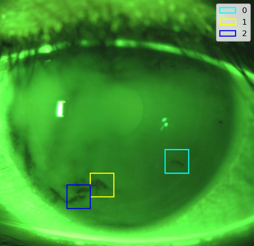
Figure 1: At left is one frame from the video of a trial, showing fluorescent intensity in green and
the locations of likely TBU instances as boxes. Right shows the intensity time series captured for
the marked boxes.
2.3 Time series extraction
Within each ROI, the images at each time were downsampled and subjected to a slight Gaussian
blur, and a location was chosen within the ROI to sample the pixel intensity of the blurred image;
details appear in Appendix C.
Figure 1 shows example results of FL intensity data extraction for a single trial. The top
left shows an image from late in the trial with likely TBU boxes marked, while the other plot
shows intensity time series from the identified ROIs. As can be seen from the plots, the shape
of the intensity curve can vary from one TBU instance to the next, even within the same trial.
This phenomenon is not unexpected, since examples of different TBU mechanisms from the same
subject have been reported in, e.g., simultaneous imaging experiments [50].Fitting ODE models of TBU 8
2.4 Model fitting
2.4.1 Models
A sketch showing the ingredients of the non-dimensional model are shown in Figure 2. Evaporative
Figure 2: Sketch of ingredients in ODE models. The film is spatially uniform. It may be subject
to loss of water via evaporation, supply of water due to osmosis, and to divergent flow away from
the middle of the film. The thickness is given by h(t).
loss of water is given, in dimensionless form, by the constant Je = v. The dimensionless supply
of water from osmosis, which may result from hypertonicity due to evaporation, is given by Jo =
Pc (c − 1). Here Pc is a dimensionless permeability and c is the osmolarity. The divergent flow is
given by the velocity field u = g(t)x, and the strain rate ∂u/∂x = g(t) characterizes the flow. This
flow is constant throughout out the thickness of the film, but varies along its length; the fluid is
simply being stretched.
We model TBU using a hierarchy of ODE models[12, 60] represented as a system of nondimen-
sional equations:
dh
= −g(t)h + Pc (c − 1) − v, (1)
dt
d(hc)
= −g(t)hc, (2)
dt
for 0 ≤ t ≤ 1, after rescaling time by a scale ts . Here the unknowns are h(t), the TF thickness, and
c(t), the osmolarity. The dependent variables are normalized so that h(0) = c(0) = 1. These values
are found by scaling the dimensional variables (primed) with
h0 c0
h= , c= , (3)
h0 c0
where h0 is the initial film thickness and c0 is the isotonic osmolarity.Fitting ODE models of TBU 9
The function g(t) accounts for transverse flow and may take one of the following three functional
forms:
Model O: g(t) ≡ 0, (4a)
Model F: g(t) = a, (4b)
Model D: g(t) = b1 e−b2 t . (4c)
The values a, b1 , and b2 are considered constant parameters. In Model O there is no fluid flow,
so the model incorporates only evaporation and osmolarity. Model F adds constant extensional
flow, while Model D allows extensional flow that decays to zero. Note that each model in (4) is
a generalization of the models above it. We also considered an additional generalization allowing
extensional flow that decays from one nonzero value to another (g(t) = a + b1 e−b2 t ), but we do not
report corresponding results due to relatively poor identifiability of its parameters for some of the
data.
The parameters v, a, b1 , and b2 (to the extent present) completely specify a model, and the
dimensional versions are optimized to fit experimental FL intensity data. The parameters are
nondimensional and related to their dimensional (primed) counterparts by
ts v 0
v= , a = ts a0 , b1 = ts b01 , b2 = ts b02 , (5)
h0
where ts and h0 are characteristic time and length scales, respectively. In practice, we choose ts
as the duration of the observation window and h0 as the initial thickness of the TF. We also have
Pc = (Po Vw c0 )/(h0 /ts ), where the dimensional permeability of the corneal surface, Po , is fixed,
Vw is the molar volume of water, and c0 is the isotonic osmolarity. Values for these dimensional
parameters are given in the appendix. The permeability Po is not a parameter in the optimization
because it is fixed[15]; however, Pc can vary while the other parameters are optimized. Parameter
values are given in Appendix B.
This spatially-uniform model allows us to obtain the nondimensional FL concentration f (t)
from scaling the osmolarity via
f (t) = f0 c(t), (6)
and the FL intensity from the film thickness and FL concentration via
1 − exp[−φh(t)f (t)]
I(t) = I0 , (7)
1 + f (t)2
where I is FL intensity and φ is the (nondimensional) Napierian extinction coefficient [14, 77].
Similarly to Pc , we have φ = f h0 fcr , which includes the dimensional extinction coefficient f (value
given in Appendix B). The value of φ varies from trial to trial because h0 does. The constant I0 is
used to match the initial observed intensity in the experiment. Scaling both the experimental and
theoretical FL intensities to start with unit value is desirable for the fitting to be described next.Fitting ODE models of TBU 10
2.4.2 Fitting
For each video recording, the procedure of Wu et al.[109] was used to estimate initial film thickness
h0 and initial fluorescein concentration f0 . We excluded as unreasonable all cases for which h0 is
outside the range 1 µm to 10 µm or f0 > 0.35%. We use f0 as the ratio between nondimensional
osmolarity and FL concentration throughout the fit. The permeability parameter in (1), Pc , varies
during the optimization as discussed in the previous section (see also Luke et al. (2021) [60]).
We excluded any intensity time series that showed substantial, sustained brightening; while
this may happen in vivo [50], we aim to fit thinning and TBU processes. Within each time series,
instantaneous values that were local outliers were removed, and the time series was smoothed
using an averaging filter. An iterative procedure was then used to isolate a window of steepest
average decrease lasting at least 3 seconds and excluding initial increases and final increases or
plateaus. This window was judged to find the regime of thinning that the ODE models are best
able to explain. The intensity values were normalized by the initial value so that I(0) = 1 and we
determined I0 in (7) to do that.
Given the normalized time series Ik at times t0 = 0, t1 , . . . , tN = 1, the objective function for
fitting ODE parameters was defined as the sum of squares,
N
1 X 1
[I(tk ) − Ik ]2 = ||I(tk ) − Ik ||22 , (8)
N N
k=0
where I(t) is from (7), using the solution of (1)–(2) and (6) for h(t) and f (t). This objective
was minimized over evaporation rate v and the constants a, b1 , b2 available in whatever form is
chosen for g(t). Constrained minimization was performed using both the BFGS and Nelder–Mead
algorithms to confirm that the same minima were reached. The dimensional forms of the parameters
were constrained to physically plausible ranges: v 0 from 0 µm/min to 40 µm/min, a0 from −1 s−1 to
2 s−1 , b01 from −1 s−1 to 5 s−1 , and b2 from 0 s−1 to 2 s−1 .
If, during ODE solution at a particular set of parameters, the numerical solution satisfied the
˙ > 0 over a sustained time interval, the solver was interrupted, and the
conditions ḣ(t) > 0 or I(t)
optimization was given a penalty value to force selection of different values. We made this choice
because the models were designed for thinning of the TF. Each optimization was attempted from
multiple initializations in order to explore the global parameter space.
Figure 3 shows fitting results for a particular ROI. Figure 3(a) shows that models F and D
fit the data much better than does the evaporation-only model O. Figure 3(b) shows that the
better models incorporate convergent flow to replace fluid lost to evaporation, which moderates the
thinning (Figure 3(c)) but increases the osmolarity (Figure 3(d)). While model O found an optimal
v 0 at 7.72 µm/min, models F and D found v 0 = 17.8 and 20.0 µm/min, respectively, indicating the
dominance of evaporation in the thinning.
Figure 4 shows fitting results for a different ROI. Here, model D is clearly superior, allowing a
significant initial divergent flow that decays away. In this case, model O found v 0 =10.0 µm/min,
while the other models found v 0 ≈ 0. The osmolarity barely increases at all when flow is active
(F or D), in contrast to the evaporative case. The fluorescein concentration barely budges as well
(proportional to the osmolarity), so the intensity change is due almost exclusively to the change inFitting ODE models of TBU 11
(a) (b)
residual norm 0.2
90
strain rate (1/sec)
0.1
80
intensity
O F D
70 0.0
60 −0.1
−0.2
2 4 6 8 10 2 4 6 8 10
time (sec) time (sec)
(c) (d)
2.4 800 0.46
fluorescein conc. (%)
osmolarity (mOsM)
thickness (μm)
700 0.41
2.2
600 0.35
2.0
500 0.29
1.8
400 0.23
1.6
300 0.17
2 4 6 8 10 2 4 6 8 10
time (sec) time (sec)
Figure 3: Results of fitting to a ROI with evaporation-dominated thinning. (a) FL intensity time
series data (dots) and the best fits of the model types O, F, and D. The bar graph shows the relative
residual norms of the fits. (b) The strain rate g(t), showing a convergent flow in the models that
allow it. (c) TF thickness in the three models. (d) Osmolarity and fluorescein concentration.Fitting ODE models of TBU 12
(a) (b)
residual norm 0.2
90
strain rate (1/sec)
0.1
80
intensity
O F D
70 0.0
60
−0.1
50
40 −0.2
3 6 9 12 15 3 6 9 12 15
time (sec) time (sec)
(c) (d)
4.5
fluorescein conc. (%)
osmolarity (mOsM)
500 0.45
thickness (μm)
4.0
3.5
3.0 400 0.36
2.5
2.0
300 0.27
3 6 9 12 15 3 6 9 12 15
time (sec) time (sec)
Figure 4: Results of fitting to a ROI with flow-dominated thinning. (a) FL intensity time series
data (dots) and the best fits of the model types O, F, and D. The bar graph shows the relative
residual norms of the fits. (b) The strain rate g(t), showing a divergent flow in the models that
allow it. (c) TF thickness. (d) Osmolarity and fluorescein concentration.Fitting ODE models of TBU 13
thickness (see (7)).
Because the models form a hierarchy, the final residuals of the models must satisfy Model O
≥ Model F ≥ Model D. As a result, the optimization of Model D was always best, and so results
below are reported in terms of its parameters. Those parameter values can change dramatically
between different instances of thinning and/or TBU.
3 Results
In total, 467 time series were successfully fitted to mathematical models. We begin discussing those
cases by examining the initial conditions found for the analysis.
3.1 Initial conditions for fitting
We compare the distribution from the current results with other mathematical models and direct
measurements of TF thickness. Creech et al. [28] used the coating flow model of Wong et al. [108]
to estimate the thickness of the deposited TF from the opening phase of the blink. Our initial
estimates for thickness are close to those of published measurements [76, 104], and appear closer
to those experiments than other methods of estimating it [28]. Figure 5 shows histograms of the
probability of the thickness from four sources, including the results from this work. One can see
that our pre-corneal tear film (PCTF) thickness estimates from fluorescein data agree well with the
80 interferometric measurements of Nichols et al. [76]; that study discussed the possible sources of
discrepancy with the relatively broad distribution of 20 no-lens estimates from Creech et al. [28]
based on coating flow theory. The 20 manual PCTF thickness estimates of Luke et al. [60] (not
shown) form a narrow distribution that is easily within the experimental range [76].
The initial thickness estimates require estimates of the initial fluorescein concentrations. These
are computed using the approach of Wu et al. [109]. The estimates for all subjects are shown in
Figure 6. The upper part of the figure shows two peaks in the histogram. Trials most often begin
close to the critical concentration of 0.2 %, which is the location of the right peak. The left peak,
around 0.1 %, is due to the protocol for the experiments. FL is not instilled for every trial so that
one or two trials could occur before additional FL is instilled; tear turnover would reduce the FL
concentration [105]. The lower part of the figure shows a scatter plot of the initial thickness and
the initial FL concentration. The two do not appear to be correlated; the initial thicknesses seem
uniformly spread across its range of values for all values of f0 . As mentioned above, the distribution
of thicknesses estimated from the f0 in Figure 5 agree quite well with measured distributions of
thickness [76].
3.2 Mechanism for all subjects
Figure 7 shows the results of all the fits as a scatter plot and marginal distributions of dimensional
evaporation rate v 0 and initial flow rate b01 , with dot sizes indicating the final osmolarity value in
the fitted model. The majority of the evaporation rates are at or below 2 µm/min, which agrees
well with interferometric measurements of central cornea thinning rates [76] and previous fitting
work [60]. The specific choice of 2µm/min was taken from the distribution of PCTF thinning ratesFitting ODE models of TBU 14
0.5 Creech et al. (1998), n=24
probability
0.4
0.3
0.2
0.1
0.0
0.5 Nichols et al. (2005), n=80
probability
0.4
0.3
0.2
0.1
0.0
0.5 this work, n=467
probability
0.4
0.3
0.2
0.1
0.0
0 5 10 15 20 25
h₀ (μm)
Figure 5: The probability distributions of initial TF thickness estimates from three sources: Creech
et al. [28] (n = 24), Nichols et al. [76] (n = 80) using interferometry, and this work (n = 467).Fitting ODE models of TBU 15
0.15
probability
0.10
0.05
0.00
0.1 0.2 0.3
initial FL concentration (%)
10
8
h0 (¹m)
6
4
2
0.1 0.2 0.3
initial FL concentration (%)
Figure 6: Top: Distribution by probability of estimated initial Fl concentrations f0 over all trials.
Bottom: Initial thickness h0 vs f0 over all fitted locations. The value of f0 is the same for an entire
trial, but h0 can vary between locations within a trial.Fitting ODE models of TBU 16
in Nichols et al [76], which showed a transition from a highly peaked set of low rates to a broad set
of higher rates.
A key question for the models is the relative importance of evaporation rate and tangential flow.
We use the flow parameter b01 , which is the initial strength of the tangential flow, as the indicator
of the importance of flow. Large positive values indicate that divergent flow is important in tear
thinning [62, 111], while a negative value indicates a convergent flow consistent with evaporation
being a primary mechanism in thinning and TBU [16, 82]. Figure 7 also shows lines drawn at
2 µm/min for evaporation and the median value 0.038 s−1 for flow, partitioning the plot into four
quadrants. The upper-left quadrant features TBU with low evaporation and strong divergent
flow, suggesting that Marangoni-driven thinning dominates; a significant fraction of these cases
seem to have little evaporation involved. The lower-right quadrant contains high-evaporation cases
featuring little flow or an initially convergent flow whose strength generally increases with the
evaporation rate. This scenario is consistent with inward tangential flow that tries to mitigate rapid
evaporative loss [16, 61, 82]. The upper-right quadrant could be interpreted as mixed-mechanism,
where both evaporation and outward tangential flow cooperate to thin the TF. The lower-left
quadrant represents cases that may not have enough thinning of either type to be definitively
called TBU; we labeled these cases “good tear film” or gtf.
It is clear from Figure 7 that the osmolarity increases with the evaporation rate, and the
relationship is plotted explicitly in Figure 8. For reference, we note that normal tear film osmolarity
measured from the inferior meniscus is somewhat variable [39, 45, 101], reportedly averaging 301
mOsM in normal subjects, with diagnostic cutoffs for DED ranging from 305-318 mOsM [45, 52,
101, 102]. However, a previous study suggests that the levels of tear film hyperosmolarity over
the cornea could be as high as 800-900 mOsM [58], much higher than the levels measured from
the inferior meniscus [45, 52]. In this study, the increase appears to be roughly linear for v 0 below
10 µm/min, but then the osmolarity tends to level off and does not exceed 950 mOsM for this set of
results. This trend agrees with previous fitting results on fewer TBU instances [60, 62] and models
with strong outward flow [110]. Previous theories of TF thinning and TBU that were not fit to
experimental data could give higher final values of the osmolarity [15, 16, 82]. The distribution of
final osmolarity values shows that for these healthy subjects, the osmolarity remains below sensory
threshold levels (450 mOsM[58]) in the majority of cases.
Figure 9 shows a scatter plot of the final osmolarity vs the initial strain rate b01 for all subjects.
The final osmolarity is negatively correlated with flow: many more hyperosmolar endpoints appear
for low flow, and relatively few for stronger flow. Fewer hyperosmolar endpoints at high flow may
be expected, but the wide range of osmolarity that may occur at moderate or low flow is again
apparent in these results.
The negative correlation observed for v 0 and b01 help explain the results in the osmolarity. There
are relatively few cases where flow is important for larger v 0 , and so osmolarity is expected to
become large in more of those cases. What may be more surprising is that there is quite a range
of flow strength for 2 ≤ v 0 ≤ 20µm/min, and this causes a relatively wide range of values in
the osmolarity for that range of v 0 . There is an overall trend, but the flow and evaporation can
cooperate to give high osmolarity in relatively short times, particularly for v 0 ≤ 10µm/min. This
was seen in previous models to some degree [60, 62], but with the current results this trend is moreFitting ODE models of TBU 17
0.25
0.15
0.05
0.2
0.1
initial flow rate (1/s)
0.0
-0.1
-0.2
0 10 20 30 40 0.02 0.06 0.10
evaporation rate (μm/minute)
Figure 7: Scatter plot of evaporation and flow rates found from model-D fits to the data. The area
of each dot is proportional to the final osmolarity predicted by the model. Marginal histograms
show the distributions in probability of each parameter. The orange lines, drawn at 2 µm/min
for evaporation and the median value 0.038 s−1 for flow, are used to color each sample to indicate
high/low rates of evaporation and flow.Fitting ODE models of TBU 18
0.25
0.15
0.05
1000
final osmolarity (mOsM)
800
600
400
0 10 20 30 40 0.05 0.15 0.25 0.35
evaporation rate (μm/minute)
Figure 8: Scatter plot of evaporation rates v and final osmolarities ce found from model D fits to the
data for all subjects. Marginal histograms show the distributions in probability of the individual
quantities. The coloring of the dots is the same as in Figure 7, indicating low/high values for
evaporation rate and initial flow.Fitting ODE models of TBU 19
0.10
0.05
1000
final osmolarity (mOsM)
800
600
400
-0.2 -0.1 0.0 0.1 0.2 0.05 0.15 0.25
initial flow rate (1/s)
Figure 9: Scatter plot of initial flow rate b1 and final relative osmolarity ce found from model D
fits to the data for all subjects. Marginal histograms show the distributions in probability of the
individual quantities. The coloring of the dots is the same as in Figure 7, indicating low/high values
for evaporation rate and initial flow.Fitting ODE models of TBU 20
0.10
0.06
0.02
1000
final osmolarity (mOsM)
800
600
400
0.2 0.4 0.6 0.8 1.0 0.05 0.15 0.25 0.35
relative final thickness
Figure 10: Scatter plot of relative final thicknesses he /h0 and final osmolarities ce found from model
D fits to the data for all subjects. Marginal histograms show the distributions in probability of
the individual quantities. The coloring of the dots is the same as in Figure 7, indicating low/high
values for evaporation rate and initial flow.
dramatic. It is clear from these results that one cannot reliably estimate the final osmolarity from
the TBU time alone; one needs knowledge of the local evaporation and flow conditions to get that
estimate.
Figure 10 shows a scatter plot and histograms for the final osmolarity ce and relative final
thickness he /h0 . The high-flow cases (red and purple dots) are correlated with lower final osmolarity,
but there is no clear association with the final thickness. We also note that the fit interval here
may not extend to full thickness TBUT in many cases. This is because the parameters can be
strongly affected if the fit interval is too long or a late plateau of low intensity is included, and for
that reason, the fit intervals could not be left too long.Fitting ODE models of TBU 21
–dh/dt, Nichols et al. (2005), n=80
0.4
probability
0.3
0.2
0.1
0.0
evaporation rate, n=467
0.4
probability
0.3
0.2
0.1
0.0
average -dh/dt, n=467
0.4
probability
0.3
0.2
0.1
0.0
0 10 20 30 40
thinning rate (μm/min)
Figure 11: Comparison of thinning rate and evaporation distributions from three sources experi-
mental thinning rate −dh/dt (with thickening in two cases) from Nichols et al. [76], as measured in
a central cornea spot of 0.2 mm diameter; evaporation rate v 0 from this work; and average −dh/dt
from this work. See text for details.
3.3 Evaporation and thinning comparisons
Figure 11 shows a comparison of thinning-rate and evaporation-rate results from the current work
with experimental results [76]. The experiment used narrow-band interferometry to measure thick-
ness rates centrally in a 0.2 mm diameter spot; thinning rates were computed from the slope of a
best fit line that began 2 s after a blink. The distribution of the measured thinning rates is within
the values we found by fitting models to FL intensity decrease. The evaporation rates we report do
yield larger values than the thinning rates in experiment. However, we note that the experiment
can only detect intensity change with time, and it cannot separate the evaporative and flow-related
contributions to TF thinning. Evaporative TBU can exhibit convergent tangential flow [16, 82],
which can significantly slow thinning. Thus, it may be expected that evaporation rate could (and
perhaps should) exceed the thinning rate in such cases.Fitting ODE models of TBU 22
0.2 1 6 11 15
0.1
0.0
-0.1
-0.2
0.2 17 18 21 22
0.1
0.0
-0.1
-0.2
flow rate (1/sec)
0.2 23 26 27 28
0.1
0.0
-0.1
-0.2
0 10 20 30 40 0 10 20 30 40 0 10 20 30 40 0 10 20 30 40
evaporation rate (μm/min)
Figure 12: Scatter plots of evaporation v 0 (abscissa) and strain rates b01 (ordinate) separated by
experimental subject. Three subjects who had fewer than 20 fits each have been omitted. Cases
marked by a cross had a final osmolarity value above the 450 mOsM threshold of discomfort.
The orange lines and symbol colors have the same meaning as in Figure 7.
3.4 Results by subject
Figure 12, like Figure 7, shows the fitting results for evaporation rate v 0 and initial strain (flow)
rate b01 , but plotted separately for each experimental subject. The plots also use a cross symbol
to indicate the cases in which the final osmolarity exceeded the 450 mOsM discomfort threshold
[58]. The orthogonal lines in each subplot show the boundaries that we chose between the different
mechanisms. High evaporation rate cases are to the right of the vertical line at v 0 = 2µm/min; high
flow cases are above the horizontal line at the median value of b01 , which is 0.038 s−1 (computed
over all trials and instances). The coloring scheme for the symbols is the same as in Figure 7.
No subject displayed exclusively high-evaporation TBU, while a few were characterized by low
evaporation rates. Most of the low-evaporation, low-flow cases that may indicate good TF occurred
in just three subjects. All subjects displayed some cases of both positive (divergent) and negativeFitting ODE models of TBU 23
subject evap flow mixed gtf total
26 25 14 7 5 51
15 14 24 6 0 44
1 16 12 14 1 43
23 20 7 10 5 42
6 12 8 7 13 40
28 13 6 2 17 38
22 20 13 2 0 35
11 5 18 10 0 33
21 10 16 6 0 32
18 13 10 8 0 31
27 13 7 6 3 29
17 11 2 11 2 26
2 4 3 0 10 17
10 0 0 2 1 3
14 0 1 2 0 3
all 176 141 93 57 467
Table 4: For the 15 subjects that were fit, there were four possible mechanisms: evaporative
(evap), flow, mixed (evaporation and flow) and good TF (gtf). The distribution of mechanisms
for all instances fit is given for each subject in descending order of number of instances fit. We
excluded the last three subjects from any subject-specific analysis because of the few instances of
TBU fit.
(convergent) initial transverse flow, at rates dispersed rather widely in most cases. It was fairly
common to exceed the discomfort threshold due to high evaporation marked by convergent flow,
while it was less common to exceed the threshold with high divergent flow.
Table 4 shows results for the healthy subjects we studied. The table is in descending order of
number of instances fit for each subject. The four possible mechanisms are that (i) evaporation
drives TBU; (ii) flow drives TBU; (iii) a mix of evaporation and flow drives TBU; and a “good
TF” (gtf) where neither evaporation nor flow is very strong. The results show that on a population
level, evaporation is the most common driver of TBU. The second most common instance is flow,
which has both small evaporation and relatively large flow rates. The relative position with respect
to v 0 = 2µm/min and b01 = 0.038 s−1 divided instances into these four classes; if greater than these
threshold values, the effect was important, and vice versa if less.
We found that perturbing these threshold values around these points did not affect the relative
distribution of the mechanisms very strongly. However, there is still some dependence on the choice
of the boundaries. For example, if we used the overall median values for both v 0 and b01 , then the
number of evaporation driven and flow driven instances are equal, and the number of mixed and
gtf cases are equal but at about half the number of the other categories. While using the median
clearly has statistical rationale, we found experimental motivation for our choice of a different v 0 .
In contrast, there is no experimental guidance for b01 since there are no direct measurements of flowFitting ODE models of TBU 24
in thinning, so we used this statistically-based choice for this parameter.
From Table 4 we also see that the distribution of mechanisms may be different from subject to
subject. For example, subject 26 has a preponderance of evaporative TBU cases, while subject 15
has a preponderance of flow TBU mechanisms. Furthermore, subjects 6 and 28 have a large fraction
of gtf cases. This suggests that, in some cases, it is possible to distinguish subjects based on their
TBU mechanism distribution. Though the specifics numbers may change for different mechanism
selection criteria, the distribution of values will still typically vary from subject to subject.
Figure 13 uses scatter plots to show the locations of every fitted TBU instance for each of the
12 experimental subjects with at least 20 total fits. The location of each dot is relative to a box
approximately enclosing the average detected cornea throughout its experimental trial; however,
the cornea does not have fixed position within the box during a trial or between different trials.
The color of each dot is used to indicate the fitted model’s final value of the osmolarity, with cases
above the discomfort threshold colored red. Each subject exhibited some potentially painful TBU
instances, which is consistent with the instructions given to the subjects in the experimental trials.
Because this data came from sustained tear exposure (STARE) trials, this distribution represents
the stimulus to the cornea in life outside the clinic.
4 Discussion
In this paper, we have employed established methods of fitting mathematical models to FL intensity
data [60] and applied them to automatically identified thinning or TBU regions in healthy subjects.
We modified the approach of Su et al. [97] to identify multiple TBU regions of interest in each trial.
With those automatically identified thinning regions, we had 12 subjects with a significant number
of TBU instances over 2 visits and 10 trials (though no subject yielded fits from all trials). The
mechanisms for each thinning and TBU is determined from the optimal coefficients from fitting
the FL intensity data. We find that each subject has a range of mechanisms associated with their
sample of TBU instances, and those distributions of mechanism may be sufficient to distinguish
between subjects. By pooling the results from all of the subjects, we have a relatively large sample
of 467 instances of thinning or TBU from 15 subjects.
A primary result is that the final osmolarity varies widely across the set of thinning or TBU
instances that we studied. This appears to happen for most subjects individually as well as for
the pooled instances. For very rapid thinning with little evaporation, or instances that turn out
to thin very little, the final osmolarity stays low. For instances that are driven by evaporation or
mixed mechanism, the final osmolarity rises to as much as 750 mOsM except for uncommon values
reaching over 900 mOsM. Because these results vary by subject, the results have the potential to
distinguish between subjects.
The results in this paper expand on prior efforts to fit FL intensity data in TF thinning and
TBU. PDE models showed the potential to fit the intensity TBU instances in some cases [16, 111],
and to determine mechanisms that drive thinning and TBU [61, 62]. Simplifying to local ODE
models of TBU allowed for faster computation and freedom to select more instances of TBU; 20
instances were fit by ODE models in Luke et al [60]. The data in this paper confirmed previously
observed trends [60] with more than 20 times the instances fit. We are unaware of other work thatFitting ODE models of TBU 25
1 6 11 15
17 18 21 22
23 26 27 28
300 450 965 mOsM
Figure 13: Scatter plots showing the locations of every fitted TBU for each of the top 12 subjects.
Each spot is located relative to a box fitted approximately around the cornea throughout the trial;
the data and squares are shifted and stretched slightly for alignment in this figure, and the position
of the cornea within the box is not constant during a trial or between different trials. The color
shows the model’s final value for osmolarity, with gray for values below the discomfort threshold of
450 mOsM [58] and increasing saturation of red for values above the threshold.Fitting ODE models of TBU 26
fits the dynamics of TBU with mathematical models or estimates the parameters within TBU at
this scale.
Experimental measurements of initial tear thicknesses include a range of approximately 2 to 10
µm using interferometry [51, 76] and similar values from optical coherence tomography (OCT) [104].
The distribution of our initial thickness estimates matches those of interferometry measurements
very well. The values found via estimation in Creech et al. [28] give a wider range of thicknesses
and a substantial fraction of thicker film estimates. Dursch et al. [35] fit a model to the thinning
and the temperature of the TF to estimate the evaporation rate of the TF. To our knowledge, they
did not determine the osmolarity of the TF in TBU, but they did use imaging data from both FL
intensity and thermal imaging to determine TF parameters of interest.
We now turn to the strengths and weaknesses of our approach. The method identifies multiple
instances of thinning and/or TBU from each trial. The system uses a trained CNN to find regions
of interest from which minimum values of intensity in the ROI are extracted throughout the trial.
The training of the CNN used labeled images with a fixed threshold of intensity for TBU across all
trials; the overall intensity of the trials varied, however, so it would likely expand the number of
trials that could be analyzed to make that threshold for TBU trial dependent. The ROIs are found
near the end of the trial, and this approach assumes that the thin regions are not moved around
by flow. However, it is possible that thinning begins elsewhere and flow moves the thinning spot
into the ROI during the first seconds of the trial [50]; this type of dynamic is beyond what our
model can analyze at this time. Extracting the minimum intensity additional Gaussian blurring
in the ROI gives acceptable FL intensity data for fitting; however, the data is noisy even after the
Gaussian filtering and smoothing. There are other possible choices of method for extracting the
intensity data, but our approach did not seem to be too sensitive to what we attempted. Some
instances have rather little happening, but are relatively dark compared to their surroundings. One
could ask whether any “good TFs” should have been selected for fitting. It is unclear at the time
of writing whether this should be the case or not; a rather long trial looks like nothing is happening
but eventually TBU may occur, yet would still be rated as a good TF. Not all trials or subjects can
be analyzed by the automatic system for TBU. This may be caused by lack of an inferior meniscus
for estimating FL concentration, failure of the initial thickness estimate, poor recording of intensity
data due to subject movement or to image focus, or possibly other reasons. The relatively low
number of subjects could also be considered a limitation of the study.
Fluorescein is used for imaging which may impact TF dynamics [22, 70, 72]. The initial FL
concentration estimates show some systematic variation, possibly because two to three trials were
performed between each FL installation. It is not clear whether a different installation protocol
may improve our method. The variation in initial FL concentration did not pose any difficulty for
estimating the initial thickness in the cases that were fit by the models, and may reduce variation
between visits that may affect other tests such as TBUT determination [26]. The use of STARE
trials does not represent healthy blinking but it does ensure that thinning and TBU occurs.
Despite these limitations, the method has produced repeatable data for hundreds of instances
of thinning and/or TBU. The data reveals trends in the conditions experienced by a cohort of
healthy TF subjects. According to the model, within TBU the final osmolarity is highly variable
due to the differing mechanisms driving TBU; this is lower than the upper limit suggested by someFitting ODE models of TBU 27
previous models without fitting [15, 16, 82], higher than flow driven models initially suggested
[111] and agrees with previous models that fit FL intensity [60]. The final osmolarity may be high
within TBU but appears to stay below 950 mOsM for this set of subjects, in agreement with the
result of Liu et al [58]. The evaporation and thinning rates appear to agree well with published
data [76], and the relationship between evaporation rate and final osmolarity is revealed to be
generally increasing with evaporation rate but is complicated by the dependence on flow. The
model determines optimal flow and evaporation values and the direction of flow (from the sign of
b01 ) is a major part of determining the mechanism of an instance.
The DEWS II Diagnostic Methodology report [107] recommended using non-invasive TBUT to
help diagnose DED rather than fluorescein due the variations induced by the latter [23, 24, 70].
The utility of each type of method is still an active area of research [72, 81, 93]. Many of these
approaches average the results of two or three measurements, and may eliminate outlying values,
as suggested by Cho et al. [23] and many others. Recent efforts have tried to automate TBUT
determination [97] and DED diagnosis [85]. The study of Segev et al. [88] found breakup times
based on mean values of aqueous layer thickness from two 40s trials separated by 45 min on average.
We note that our approach is not aimed at using TBUT as a method for diagnosis; we are refining
the use of FL imaging to yield the mechanism driving thinning and TBU for many instances in
each healthy subject. We are attempting to find the distribution of what can occur within healthy
subjects, and there appears to be significant variability within each subject and even within a single
trial. We are unaware of prior studies that investigated within-subject TBU variability. This basic
science data may have clinical application in classifying subjects based on their thinning and/or
TBU characteristics.
Some studies have noted and tried to exploit the distributions of tear film parameters to distin-
guish between subjects. An example is Bai et al [5] where optical microscopy is used to measure the
LL thickness for healthy subjects and several conditions related to meibomian gland dysfunction.
The distribution of LL thickness over a small area is analyzed for each subject and differences
between conditions can be seen from these distributions.
In this study, we identify parameters and mechanisms for multiple instances of thinning in each
subject. Those instances present varying amounts of chemical, thermal and mechanical stimuli to
the ocular surface. The mechanism by which those stimuli are sensed or received, and the role of
that perception in DED, is a matter of ongoing research [9]. Various neural receptors are thought
to play important roles in sensing these different stimuli: chemical [9], thermal [44, 80, 92], and
mechanical [3, 7]. While our work here cannot directly address such questions, we believe that
quantifying the stimulus at the ocular surface can only help to clarify such processes.
In order to compute the fits to the extracted data, reasonable ROIs for extraction must be found
in each trial. For the healthy subjects that we used, less than half of the trials yielded ROIs for
analysis. Improving the robustness of the ROI detection would be an efficient way to generate more
data to characterize thinning and TBU instances and the subjects in which they occur. Once ROIs
are determined, there may be other options than what we employed for extracting the thinning
data. The FL images were somewhat noisy, and despite filtering to minimize it, extracting local
data may be affected by that noise.
The estimates of initial FL concentration, and subsequently the initial thickness, required aFitting ODE models of TBU 28
special procedure with low illumination intensity and a good inferior meniscus. This may limit the
trials and subjects that may be analyzed. Other possible ways to estimate these initial quantities
may improve robustness of the method. The method appears to work very well when estimates can
be obtained, based on comparison with interferometric in vivo results.
5 Conclusion and future perspectives
An important next step would be to apply the method to a sample of DED subjects to compare
with the data from healthy subjects. Combining our method with data from simultaneous thermal
imaging[35], interferometry[50], or sensory feedback and/or sensory response [3, 57, 58] could yield
new insights.
A Model Derivation
Consider a rectangular control volume of −L0 /2 ≤ x0 ≤ L0 /2 and 0 ≤ y 0 ≤ h0 (t0 ); this rectangle
could be centered on Figure 2. The equations result from conserving solvent (the aqueous layer’s
water) and solutes (osmolarity, c0 , and fluorescein concentration, f 0 , both in M) per unit width of
the film. The water conservation is given by
dh0
ρL0 = −Je0 L0 + ρPo Vw (c0 − c0 )L0 − 2ρh0 u0 (L0 /2, t0 ) (9)
dt0
where the (constant) evaporation rate is given by Je0 = ρv 0 . The term on the left is the rate of
change of the mass of water in the control volume. The first term on the right is the water lost
due to evaporation; the second term is supply of water due to osmosis. The remaining term is the
total amount of water flowing out of the ends from a depth-independent velocity field u0 (x0 , t0 ) =
g 0 (t0 )x0 ; this velocity along the film is evaluated at x0 = ±L0 /2. The time dependence is given by
0 0
g 0 (t0 ) = b01 e−b2 t .
Conservation of solutes is given by
d(h0 s0 )
L0 = −[2u0 (L0 /2, t0 )]h0 s0 , (10)
dt0
where s0 = c0 or f 0 . The term on the left is the rate of change of solute in inside the control volume,
and the term on the right is the total amount of solute leaving the sides of the control volume at
x0 = ±L0 /2.
Substituting u0 (L0 /2, t0 ) = g 0 (t0 )L0 /2 into the equations and rearranging gives, for water,
dh0
= −v 0 + Po Vw (c0 − c0 ) − h0 g 0 (t0 ), (11)
dt0
and for solutes,
d(h0 s0 )
= −g 0 (t0 )h0 s0 . (12)
dt0
Substituting for g 0 (t0 ) and converting to non-dimensional variables via (3) and f 0 = fcr f results in
the nondimensional equations given in Section 2.4.1.You can also read