Modeling train route decisions during track works - Research ...

ETH Library

Modeling train route decisions
during track works

 Journal Article

 Author(s):
 Schmid, Basil ; Becker, Felix; Molloy, Joseph ; Axhausen, Kay W. ; Lüdering, Jochen; Hagen, Julian; Blome, Annette

 Publication date:
 2022-06

 Permanent link:
 https://doi.org/10.3929/ethz-b-000547324

 Rights / license:
 Creative Commons Attribution 4.0 International

 Originally published in:
 Journal of Rail Transport Planning & Management 22, https://doi.org/10.1016/j.jrtpm.2022.100320

 This page was generated automatically upon download from the ETH Zurich Research Collection.
 For more information, please consult the Terms of use.

Journal of Rail Transport Planning & Management 22 (2022) 100320

 Contents lists available at ScienceDirect

 Journal of Rail Transport Planning & Management
 journal homepage: www.elsevier.com/locate/jrtpm

Modeling train route decisions during track works
Basil Schmid a ,∗, Felix Becker a , Joseph Molloy a , Kay W. Axhausen a ,
Jochen Lüdering b , Julian Hagen b , Annette Blome b
a Institute for Transport Planning and Systems (IVT), ETH Zurich, Stefano-Franscini-Platz 5, CH-8093 Zurich, Switzerland
b DB Netz AG, Theodor-Heuss-Allee 5-7, DE-60486, Frankfurt a. Main, Germany

ARTICLE INFO ABSTRACT

Keywords: To better understand the choice behavior of train route schedulers and to predict their choices
Train route decisions for optimizing the annual construction schedule, prospective data for 2020 on train route
Construction schedule decisions are analyzed using discrete choice models and machine learning classifiers. The choice
Track works
 alternatives include (i) partial cancellation of the train schedule at the start, (ii) in the middle
Discrete choice model
 or (iii) at the end of the itinerary of the train service, (iv) detour and (v) delay/ahead of time,
Machine learning classifier
Forecasting
 and are modeled using 39 train-, construction site-, and infrastructure variables. The top nine
Behavioral outcomes attributes account for about 80% of variable importance, including the travel time from the
 departure station to the construction site, total or line closure, travel time from the construction
 site to the terminus, length of the train and effective line capacity.
 The models are tested for 2021 and 2022 to verify whether they can be used to forecast
 choices in the following years. While Random Forest performs best in terms of prediction
 accuracy (2021: 60.8%; 2022: 58.6%), the improvements of about 6%-points compared to
 the Mixed Logit model are modest. Results indicate that a substantial amount of unobserved
 construction site heterogeneity is present, which Random Forest cannot capture either.

1. Introduction

 The construction schedule is an important factor in minimizing the impact of construction-based capacity restrictions in order
to guarantee smooth rail operations. To optimize this process, the aim of this paper is to provide an empirical basis for supporting
the train route schedulers by providing likely outcomes based on current observations for five different scheduling alternatives:
Cancellation of the train schedule at the beginning (KA), in the middle (KM) and at the end (KE) of the itinerary of the train
service, detour (U) and delay/ahead of time (V). Using 39 train-, construction site-, and infrastructure attributes, statistical models
are trained for large datasets from the German Railway system (DB).
 The envisaged optimization pipeline is schematically described in Fig. 1: Once the affected trains are known in step (1) – based
on the predictions of the statistical model – perspective rules and regulations (2) are created on an annual basis. These rules are then
included in the optimization process (3) of the construction schedule (for an introduction to the automatic construction schedule
process, see discussions in Dahms et al., 2019). If a new schedule is approved by the operators concerned (4), it will be adopted
(5); if not, there will be a feedback loop re-examining the input predictions. The goal of this paper is related to step (2), trying to
better understand the choice behavior of the nationwide operating train route schedulers and to accurately predict their choices

 ∗ Corresponding author.
 E-mail addresses: basil.schmid@ivt.baug.ethz.ch (B. Schmid), felix.becker@ivt.baug.ethz.ch (F. Becker), joseph.molloy@ivt.baug.ethz.ch (J. Molloy),
axhausen@ivt.baug.ethz.ch (K.W. Axhausen), jochen.luedering@deutschebahn.com (J. Lüdering), julian.hagen@deutschebahn.com (J. Hagen),
annette.blome@deutschebahn.com (A. Blome).

https://doi.org/10.1016/j.jrtpm.2022.100320
Received 22 December 2020; Received in revised form 11 April 2022; Accepted 27 April 2022
Available online 13 May 2022
2210-9706/© 2022 The Author(s). Published by Elsevier Ltd. This is an open access article under the CC BY license
(http://creativecommons.org/licenses/by/4.0/).

B. Schmid et al. Journal of Rail Transport Planning & Management 22 (2022) 100320

 Fig. 1. Integration of results in the optimization process of the German Railway system (DB).

for the subsequent annual planning horizons. As the network is constantly evolving and interdependencies start to occur as soon
as first real-time choices are made, the forecasting models are not intended to be used in the short-term, i.e. for the actual daily
operation.1 Since the construction site schedules are created on an annual basis (see discussions in Dahms et al., 2019), they rather
should support train route schedulers’ decision-making in a longer-term planning horizon.
 The main contribution of this paper is to provide a detailed empirical analysis on the different factors affecting the choices of
train route schedulers — a completely new topic that has not yet been addressed in the field of transportation research so far.
While providing little in terms of methodological advances, the main value added of this paper should be seen from a techno-
practical perspective, providing insightful analyses and tools relevant to train route schedulers. A comprehensive investigation
of the importance of the different train-, construction site-, and infrastructure attributes is crucial to understand their behavior,
including the potential presence and amount of unobserved construction site heterogeneity. While a better understanding of the
decision-making process is mostly important from a management and communication point of view, from a technical point of view,
the main goal is to make accurate predictions about new decisions in the construction site schedule for new construction sites that
enter the optimization process. To investigate both requirements, the choices on how to deal with a train when it is affected by a
construction site are modeled using two conceptually different classification approaches: A traditional econometric and a machine
learning approach.
 A general trend is observable that machine learning approaches are being used more and more often especially for prediction
purposes (for a review of different methods, see e.g. Kotsiantis, 2007), and recent research also has made successful attempts to
combine them with traditional econometric models (e.g. Sifringer et al., 2018; Yang et al., 2018). In the field of transportation
research, the applications vary from travel behavior and mode choice prediction (e.g. Cantarella and de Luca, 2005; Omrani, 2015;
Ke et al., 2017; Sun et al., 2018; Lhéritier et al., 2019; Zhao et al., 2020), travel incident prediction (e.g. Nassiri et al., 2014;
Brown, 2015), travel time and flow prediction (e.g. Vanajakshi and Rilett, 2007; Zhang and Haghani, 2015; Xie et al., 2020) to
purpose and mode imputation (e.g. Montini et al., 2014; Feng and Timmermans, 2016) as well as pattern recognition for travel mode
and route choice prediction (for a comprehensive literature review, see also Cheng et al., 2019; Pineda-Jaramillo, 2019). Many of
them have reported a superior prediction accuracy (PA) of Random Forest (RF; e.g. Breiman, 2001; Liaw and Wiener, 2002; Cutler
et al., 2012) compared to other machine learning classifiers (for a comprehensive performance overview for different datasets, see
also e.g. Caruana and Niculescu-Mizil, 2006), and have demonstrated that RF especially outperforms the traditional discrete choice
models such as Multinomial Logit (MNL) often substantially, in some cases showing more than 20%-points improvements in PA (e.g.
Hagenauer and Helbich, 2017; Cheng et al., 2019; Zhao et al., 2020).
 Discrete choice models are based on the well-founded concept of utility maximization when modeling the choice of an
alternative (e.g. McFadden, 1986), facilitating the interpretation of results due to a transparent specification of the functional
form. The discrete choice models start with a basic specification, the MNL model, which is extended by accounting for unobserved
heterogeneity and correlated alternatives, the nested error component Mixed Logit model (MIXL; e.g. Hensher and Greene, 2003;
Walker et al., 2007; Train, 2009). Therefore, an important strength of discrete choice models is related to the possibility to
explicitly account for the panel structure. While recent papers discuss the superior PA of machine learning models also for panel
data (Zhao et al., 2020; Chen, 2021), they do not explicitly recognize the dependency structure of repeated observations. Also, one
should note that all attributes are describing the train-, construction site-, and infrastructure characteristics, which are invariant
across alternatives. Thus, including random error components is an obvious way to account for unobserved heterogeneity at the
construction site level, while random taste parameters cannot be estimated by definition (Train, 2009). Given the already large
number of parameters (39 attributes × (5 – 1) alternatives + 4 constants = 160) to be estimated even in the most basic MNL

 1 Given the workflow of the train route schedulers and the prospective creation of annual construction schedules, the dynamic aspect was not the primary focus

of this project. The main goal of the models is to predict the choices for new observations, where no prior knowledge on previous behavior or interdependencies
in the system is available.

 2

B. Schmid et al. Journal of Rail Transport Planning & Management 22 (2022) 100320

specification, other specifications such as the latent class model (e.g. Greene and Hensher, 2003) were discarded, as it would add
(up to) 160 additional parameters for each additional class.
 Given the transparency of a choice model — it is, however, subject to restrictive assumptions that usually come along with
a lower PA. In fact, the researcher typically does not know which, if any, functional form best approximates reality. In addition,
especially in the case of large datasets (as in the current case with more than 150,000 observations and 39 explanatory variables),
the estimation of MNL models is computationally cumbersome, and even more so with more advanced specifications such as the
MIXL model (e.g. Bhat, 2001). In order to be able to improve the discrete choice model specification and use a sufficient number of
random draws to guarantee stability in parameter estimates (Walker and Ben-Akiva, 2002), we simplify the models and present a
data compression method similar as in van Cranenburgh and Bliemer (2019) to effectively reduce the size of the estimation dataset.
By moving away from the main goal of maximizing out-of-sample PA, we create behaviorally richer choice models, which are later
used to calculate the marginal probability effects (MPE) and elasticities (E).
 Machine learning classifiers are used as a complementary tool to the discrete choice models mainly for the purpose of forecasting,
investigating by how much data-driven approaches may outperform the behaviorally richer choice models. Since there exists a wide
range of different classifiers (see e.g. Kotsiantis, 2007; Suthaharan, 2016), we had to narrow down the algorithms tested in this
paper. Although there is no dominant position of any classifier per se, for the current application RF is considered to be a very
promising approach. RF is known to be particularly efficient in the prediction of discrete outcomes due to the high flexibility
in functional forms (e.g. Lhéritier et al., 2019) as well as higher-order interactions (e.g. Cheng et al., 2019), is easily applicable
to very large datasets with modest computational resources (e.g. Cervantes et al., 2020), and the hyperparameters are relatively
easy to tune (e.g. Probst et al., 2019). Two commonly used, but fundamentally different classifiers that are also tested in this
paper – Support Vector Machines (SVM; e.g. Cortes and Vapnik, 1995) and Artificial Neural Networks (ANN; e.g. Bishop et al.,
1995) – typically require more efforts: SVM require to choose an appropriate kernel function as well as parameters related to the
degree of over-fitting (see e.g. Zhang and Xie, 2008). For multi-class classification, the often implemented one-against-one approach
requires to train multiple SVM (Hsu and Lin, 2002; Meyer et al., 2019), substantially increasing the computation time (see also
e.g. Suthaharan, 2016) if the number of classes increases. And especially for very large datasets, the computation time of SVM may
become excessive (Cervantes et al., 2020). ANN, in the simplest case, require to choose a weight decay parameter related to the
penalization of more complex functions (MacKay, 1999), the number of hidden layers (typically one or two) and the neurons within
each layer as well as the activation function (e.g. Wang, 2003). While many factors must be taken into account, ANN are also very
sensitive to the occurrence of noise in the training data (Cervantes et al., 2020). All methods – RF, SVM and ANN – require some
grid search techniques to come up with an appropriate specification of hyperparameters (for a discussion on tuning of all three
algorithms, see e.g. Deng et al., 2019).
 Machine learning models have in common that they are data-driven — an issue that has been shown to often undermine its
usefulness when obtaining behaviorally plausible outcomes (for discussions, see e.g. Dreiseitl and Ohno-Machado, 2002; Karlaftis and
Vlahogianni, 2011; Zhao et al., 2020). As investigated in Zhao et al. (2020), an interpretation of the MPE and E of the covariates is
only partially meaningful, since ceteris paribus interpretations (such as in the discrete choice approach) are only possible under certain
conditions and to a limited extent. In case of RF, when variables are correlated and differ in their manifestations, the importance of
variables in explaining the outcome is biased towards attributes with a higher value range (when forming the trees, more splits are
possible in the data; see e.g. Strobl et al., 2007; Nicodemus and Malley, 2009; Nicodemus et al., 2010).2 In case of ANN, multiple
model architectures may exist that perform equally well, but lead to different interpretations of results (Cantarella and de Luca,
2005). Consequently, this leads to biased conclusions not only about the importance of an attribute but also its actual marginal
effect (for further discussions about the advantages and disadvantages of machine learning versus traditional econometric models,
see e.g. Kleinberg et al., 2015; Paredes et al., 2017; Sun et al., 2018; Hillel et al., 2019). Therefore, a major aim of this paper is to
show the bottlenecks and advantages of these two conceptually different modeling approaches in terms of PA, behavioral insights
including variable importance (VI), MPE and E, as well as computing time and modeling effort, and discuss them for the specific
application of train route scheduling during track works.
 To our best knowledge, only one study has investigated the behavioral outputs and PA of machine learning classifiers and a MIXL
model using a panel dataset. Zhao et al. (2020) show that for their mode choice dataset, RF clearly outperforms in terms of PA also
among different machine learning classifiers (including ANN and SVM), while obtaining an even lower PA of the MIXL than the MNL
model (a similar result that was found in Cherchi and Cirillo (2010)). However, properly accounting for unobserved heterogeneity,
especially in the current application (on average, about 80 observations per construction site), is considered as an important issue
to be investigated, potentially affecting the behavioral outputs and PA. If the amount of unobserved heterogeneity is substantial, it
could to some extent also undermine the benefits of the machine learning classifiers when validated on new observations.
 The structure is as follows: Section 2 provides a comprehensive data overview and describes the model variables, including
a correlation analysis of all train-, construction site-, and infrastructure attributes. Section 3 presents the different modeling
frameworks and briefly discusses the related advantages and disadvantages. Section 4 presents the main results and evaluates the
differences between the MNL, MIXL, RF, ANN and SVM approach in terms of PA and VI. Furthermore, we present a data and model
simplification strategy to reduce the computational costs, which allows us to obtain the MPE and E for behaviorally richer choice
models. Section 5 summarizes and discusses the main findings, implications for practical applications and limitations.

 2 Clearly, the high flexibility in the functional form is associated with a high PA (and in many practical applications, this may be as important as causal

inference; Kleinberg et al. (2015)), though it makes interpretation difficult: If a continuous variable is correlated with a discrete attribute, it may essentially
absorb most of the effect of that attribute, making it less important.

 3

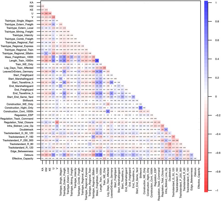
B. Schmid et al. Journal of Rail Transport Planning & Management 22 (2022) 100320

 Table 1
 Data overview for the training (2020) and the two test (2021 and 2022) datasets.
 2020 training dataset 2021 test dataset 2022 test dataset
 # construction sites 1925 2522 2633
 # choice observations 151,901 248,751 162,375

2. Data preparation and description

 Data are generated based on the German train scheduling software MakSi FM (Makro Simulation Fahrplan Modifikation), to
which the responsible train route schedulers at DB prospectively (i.e. for every planning horizon in advance, which typically covers
one year) add rules on how trains are affected when they enter a construction site. DB was collaborating with the Institute for
Transport Planning and Systems (IVT) of the Swiss Federal Institute of Technology (ETH) to investigate the key attributes and their
influences on the choices of train route schedulers.
 The data preparation mainly involved the merger of the train-, construction site-, and infrastructure attributes, where the relevant
variables and their manifestations (i.e. exact calculations, available choice alternatives, discrete vs. continuous value ranges, etc.)
were created in a continuous exchange with professionals from DB. Given that the main goal is to provide an annual forecasting
model for different planning horizons, three datasets were created for the years 2020, 2021 and 2022. In subsequent analyses, 2020
is used as a training dataset (estimation sample), whereas 2021 and 2022 are used as test datasets (holdout sample).3 As shown in
Table 1, each dataset contains more than 150,000 observations of about 2000 construction sites.
 A construction site thus typically involves multiple choices for different trains, as illustrated in Fig. 2. For all three datasets it
shows highly rightskewed distributions with an average of about 80 choice observations per construction site (note that the train
attributes may vary for each construction site, while by definition the construction site-, and infrastructure attributes are invariant).
 The relevant choice dimension involves five alternatives4 :

 • KA: Cancellation of the train schedule at the beginning of the itinerary of the train service (also includes total cancellation of
 the train schedule)
 • KM: Cancellation of the train schedule in the middle of the itinerary of the train service
 • KE: Cancellation of the train schedule at the end the itinerary of the train service
 • U: The train is redirected; it makes a detour
 • V: The train passes through the construction site with a delay or ahead of time

 As shown in Fig. 2, in all datasets U exhibits the highest relative choice frequency of more than 45%, followed by V (about 15%)
and the three cancellation alternatives KA, KM and KE.
 A complete list of train-, construction site-, and infrastructure attributes is shown in the Appendix, Table A.1, including a short
description of each variable (for summary statistics, see Appendix, Table A.2). Together with the categorical attributes such as train
type, type of the start/end yard of the itinerary of the train service, regulation at the construction site and track standard (which are
re-coded as dummy variables), in total there are 39 explanatory variables (excluding the reference categories due to identification
issues)5 that are used in subsequent analyses.
 Train-related attributes include the different train types, mass (only available for freight trains) and length of the train, when
and how much a train is affected by the construction site and information on the itinerary of the train service. Attributes related
to the construction sites mainly include information on the type of work and when it takes place, as well as the regulation at
the construction site, while infrastructure attributes mainly include information on the track operation, technological standards
including number of detours, effective capacity and edge betweenness6 of the construction site.
 To get a first idea on the dependencies within the training dataset,7 Fig. 3 shows a correlation matrix of the choice and
explanatory variables. It already indicates the sign and magnitude of effects on the choice of each alternative: The strongest
correlations exhibit variables related to the proportions of the train (Mass_Freighttrain_1000t and Length_Train_1000m), indicating
that longer and heavier (freight) trains have a lower chance of a cancellation (negative correlations with KA, KM and KE) but a
higher chance of being redirected (positive correlation with U) — a similar pattern that is found for the number of detours. The
opposite pattern is found for regional passenger trains (most pronounced for Traintype_Regional_SBahn), exhibiting a higher chance
of a cancellation while a redirection becomes less likely. On the other hand, if there is a total route closure (Regulation_Total_Closure),
the chance of a cancellation increases, while the chance of a delay (V) strongly decreases.

 3 Based on preliminary investigations, merging the 2020 and 2021 into one large training dataset has been shown to be not decisive in terms of PA for the

2022 dataset (see also discussions in Section 4.4 and results in Table 5).
 4 The original choice dimension involved one additional alternative (D: The train passes through the construction site without any changes in the timetable

and construction schedule). This alternative was removed after discussions with experts from DB, since it exhibited a very low choice frequency of 2% and was
considered as not relevant for construction site scheduling.
 5 Note that categories of categorical variables with a share below 2% in the training dataset are not modeled explicitly (i.e. added to the reference categories)

due to estimation issues in the MNL and MIXL model. This includes all categories denoted with a star in Table A.2.
 6 Edge betweenness is a measure of the relative importance of the track within the German rail network (Freeman, 1978).
 7 Note that the dependencies are very similar in the two test datasets.

 4

B. Schmid et al. Journal of Rail Transport Planning & Management 22 (2022) 100320

Fig. 2. Choice densities by alternative for the training (2020) and the two test (2021 and 2022) datasets and number of observations by construction site. KA
= cancellation of the train schedule at the beginning of the itinerary of the train service (includes total cancellation); KM = cancellation of the train schedule
in the middle of the itinerary of the train service; KE = cancellation of the train schedule at the end of the itinerary of the train service; U = detour; V =
delay/ahead of time.

 Important for the subsequent interpretation of effects are the correlations within attributes, as further discussed in Section 3.5.
Fig. 3 reveals dependencies within explanatory variables such as Mass_Freighttrain_1000t and Length_Train_1000m, as expected
exhibiting a strong and positive correlation of +0.85. Both variables are also strongly correlated with the number of available
detours (i.e. such trains are typically operated on routes with more options for diversion) and the different train types (freight
trains typically are heavier and longer, while especially regional passenger trains are smaller and shorter). It also shows that
mainly external (i.e. not belonging to DB) freight trains (Traintype_Extern_Freight ) typically follow longer itineraries of the train
service (positive correlations with Start_Traveltime_h and End_Traveltime_h) and exhibit a higher chance to leave or enter Germany
(LeavesOrEntersGermany), and that heavier and longer trains (mainly including external freight trains) are stronger associated with a
start or end in a freight or marshaling yard. Furthermore, shift work operation (Shiftwork) is positively associated with construction
during night time (Construction_Night_Only), while construction sites over multiple days (Log_Days_Train_Affected) also exhibit a longer
duration of uninterrupted operation of construction work (Construction_Cont_1000h). Most of the remaining correlations are small to
moderate (|c| < 0.5). As discussed in subsequent sections, these interdependencies are important for a better understanding of the
results of the different modeling approaches.

3. Modeling framework

 From a technical point of view, the main goal of the models is to make accurate predictions about future decisions in the
construction site schedule. Therefore, maximizing the out-of-sample PA is the main goal. From a management and communication
point of view, however, there is also a strong requirement for better understanding the choice behavior of the train route schedulers
in the sense of which attributes are most important and how they affect the choices quantitatively.
 We want to stress at this point that a profound comparison between discrete choice and machine learning models is not targeted,
as it has been done in previous research already (e.g. comprehensive work has been done by Zhao et al., 2020). The main goal is
to use both techniques in a complementary and supporting way, and in subsequent analyses put the focus on one method when
it outperforms the other (see e.g. discussions in Chen, 2021). We therefore propose a pragmatic approach by making use of the

 5

B. Schmid et al. Journal of Rail Transport Planning & Management 22 (2022) 100320

 Fig. 3. Correlation matrix of choice and train-, construction site-, and infrastructure attributes (2020 training dataset).

advantages of the different modeling techniques depending on the specific application — either as an input tool for the optimization
process (maximizing PA) or to implement policy relevant management decisions (maximizing behavioral insights).

3.1. Multinomial Logit (MNL) and Mixed Logit (MIXL) model

 The utility function of alternative ∈ {KA, KM, KE, U, V} and construction site ∈ {1, 2, … , } in each choice situation for train
 ∈ {1, 2, … , } is given by

 , , = + , + , + , , (1)

where (delay/ahead of time) is the reference alternative for identification purposes. The utility function , , includes the following
components:

 • : Alternative-specific constant (ASC parameter)
 • , : Vector of train-, construction site-, and infrastructure attributes (note that for a given construction site , train attributes
 may vary in )
 • : Alternative-specific parameter vector of train-, construction site-, and infrastructure attributes

 6

B. Schmid et al. Journal of Rail Transport Planning & Management 22 (2022) 100320

 • , ∼  (0, 2 ): Unobserved random error component in the utility function (e.g. Bhat, 1995; Walker et al., 2007) related to
 
 construction site .
 • , , : Remaining IID extreme value type I error term

 With the data structure (panel data) described in Section 2, a major issue is the violation of distributional assumptions regarding
the error terms (i.e. independently and identically distributed; IID; see e.g. Train, 2009). Observations are not independent and
unobserved factors, especially at the construction site level,8 may come into play, that – if not properly accounted for – may
lead to a bias in parameter estimates (e.g. Greene and Hensher, 2007; Baltagi, 2008), potentially affecting the interpretation and
results of behavioral outputs. Therefore, the MIXL models also include the alternative-specific random error components , . One
should note that the MIXL may not be substantially better in terms of PA than the MNL model, since for out-of-sample forecasts
the unobserved components are, by definition, unknown. Nevertheless, this additional layer of complexity may help to get more
informative parameter estimates and improve the general picture of which attributes are important and how sensitive results are
with respect to changes in the underlying modeling assumptions.
 The probability (⋅) that alternative among the full set of available alternatives ∈ {KA, KM, KE, U, V} for train passing by
construction site is chosen is given by
 exp( , , )
 ( , | , , ) = ∑ (2)
 exp( , , )

where , , is the systematic component of utility and is the vector of all model parameters to be estimated.
 Models are estimated with the -package mixl (Molloy et al., 2021), a specialized software tool for estimating flexible choice
models on large datasets. The initial MIXL model uses 100 Sobol draws to simulate the choice probabilities (e.g. Train, 2009).
Although this number is not large enough to guarantee stability in parameter estimates (Walker and Ben-Akiva, 2002), given
the large training dataset it is the maximum number with a still feasible computation time.9 Therefore, in an additional effort,
a reduced/compressed dataset is created and a model only including influential effects is estimated, using 2000 Sobol draws to
guarantee stability (RMIXL model), which is mainly used to calculate unbiased behavioral measures such as MPE and E. Cluster-
robust (by construction site ID)10 standard errors are obtained by using the Eicker–Huber–White sandwich estimator (e.g. Zeileis,
2006).

3.2. Random Forest (RF) model

 The Random Forest (RF) approach is used to classify the choice of alternative ∈ {KA, KM, KE, U, V} using binary recursive
partitioning (e.g. Liaw and Wiener, 2002; Cutler et al., 2012). It is particularly efficient for very large and high-dimensional datasets
and if one of the main goals is to obtain a high PA (e.g. Archer and Kimes, 2008; Qi, 2012). RF is relatively easy to use and mainly
requires two hyperparameters to be defined (Liaw and Wiener, 2002): The number of trees in the forest ( ) and the number of
variables in the random subset of explanatory variables for which the best split is chosen ( ). However, a more fine-grained choice
of additional hyperparameters is necessary to avoid over-fitting and increase computational efficiency. Therefore, in a preliminary
effort, different combinations of hyperparameters were tested using the -package tuneRanger (Probst et al., 2019) for , the
minimum number of observations in the terminal nodes ( ) and the fraction of the training dataset used for training of the
trees ( . ), which we did for varying . A good performance (using a parsimonious setting) was found for =
18, . = 0.86 and = 2. In a second effort, different combinations of and maximal number of terminal
nodes ( . ) were investigated. Results have shown that after = 250 and . = 1024, the out-of-sample PA (2021
test dataset) has mostly converged.11 Models are trained using the -package randomForest (Liaw and Wiener, 2002).

3.3. Artificial Neural Network (ANN) model

 The Artificial Neural Network (ANN) approach is used to classify the choice of alternative using a three-layer,12 inter-connected,
feed-forward network, aiming to minimize the error between observed and predicted choices (e.g. Bishop et al., 1995; Olden et al.,
2004; Cantarella and de Luca, 2005). The connection weights are trained using error back-propagation and a logistic activation
function with a maximum of 1500 iterations. The input layer consists of 39 neurons (i.e. one for each attribute), the second (hidden)
layer consists of a number of neurons to be defined (see below) and the third layer is the output layer relating to the choice. Based
on grid search techniques, multiple combinations of the number of neurons in the second layer, as well as weight decay parameters

 8 Examples are missing construction site and/or infrastructure attributes that may require specific regulations of trains, leading to a unobserved preferences

for certain choice alternatives.
 9 The MIXL model was estimated on the ETH supercluster Euler using 48 cores with a total CPU time of 12,326 h; see also Table 4 for CPU time comparisons

across all estimated models.
 10 Note that for numerical issues, construction sites with >150 observations were assigned to a new construction site ID.
 11 Note that increasing 
 and/or . might even reduce the PA in the test dataset due to overfitting. The hyperparameter setting in the RF models
used in subsequent analyses is summarized in Table A.4. After all, the differences in PA were small, supporting the consensus that RF in general is not very
sensitive to the exact values of hyperparameters (Liaw and Wiener, 2002), which stands in stark contrast to other machine learning classifiers such as SVN and
ANN (e.g. Deng et al., 2019).
 12 Adding an additional hidden layer (i.e. four layers in total), given any specification of hyperparameters, failed with respect to model convergence.

 7

B. Schmid et al. Journal of Rail Transport Planning & Management 22 (2022) 100320

(both are related to the degree of over-fitting) were tested (e.g. Krogh and Hertz, 1992; Smith, 2018), showing a high out-of-sample
PA (2021 test dataset) with 19 neurons and a weight decay parameter of 0.05. Models are trained using the -package caret (Kuhn,
2008).

3.4. Support Vector Machine (SVM) model

 The Support Vector Machine (SVM) approach is used to classify the choice of alternative by mapping the input vector of train-,
construction site-, and infrastructure attributes into a high dimensional feature space using a non-linear kernel function, finding
a hyperplane that optimally separates different classes by maximizing the margin between them (e.g. Cortes and Vapnik, 1995;
Cervantes et al., 2020). As discussed in Lameski et al. (2015), when the classes are not linearly separable, the choice of the cost
parameter governs how much mis-classification errors are penalized in the training dataset. Using a Gaussian radial basis function
(RBF) kernel, the parameter governs the flexibility of the decision boundary that separates the hyperplane. Based on grid search
techniques, multiple combinations of the hyperparameters were tested, showing high out-of-sample PA (2021 test dataset) for a 
parameter of 10 and a parameter of 0.01. Models are trained using the -package e1071 (Meyer et al., 2019).
 Compared to the RF approach, both the SVM and ANN models were more sensitive to the choice of tuning hyperparameters,
although the range of acceptable values could be narrowed down after some preliminary trials. However, it took substantially more
computing power to estimate the models, especially for the SVM, as presented in Table 4.

3.5. Variable importance (VI)

 When investigating the discrete choice and machine learning approaches with respect to the interpretation of results, several
important issues that are related to the ranking in VI, MPE/E and PA have to be considered. In the discrete choice model, if the
explanatory variables are correlated, the parameter estimates may still be unbiased and so are the resulting marginal effects and
elasticities, allowing a ceteris paribus (all else equal) interpretation.13 The linear-additive utility function in Eq. (1) implies a separable
and equal meta-level importance of each variable that is weighted by exactly one parameter for each except the reference alternative
(i.e. , ), no matter if is discrete or continuous. This rather restrictive setting is one of the main explanations for the lower PA
of traditional econometric models compared to machine learning classifiers (e.g. Gevrey et al., 2003; Hagenauer and Helbich, 2017;
Paredes et al., 2017). Clearly, without further adjustments, possible higher-order interactions and non-linear relationships are not
captured (see e.g. Hillel et al. (2019); if so, they have to be parametric, i.e. explicitly specified as polynomial or dummy effects, or
using other non-linear transformations, which would make model specification cumbersome especially for high-dimensional datasets
as the current one). However, the main advantage is that VI has a very clear interpretation: Ceteris paribus, attribute contributes
more to the utility of alternative if and/or , is higher (in absolute values).
 A simple and intuitive measure of VI in discrete choice models can be defined as the total average utility partworth (for the
concept of utility partworth, see e.g. Goldberg et al., 1984; Kuhfeld, 2010), given by
 ∑
 , , = | ̂ , | ⋅ | | (3)
 
where the absolute value of the estimated parameter | ̂ , | is multiplied with the sample mean of the absolute values of the
corresponding variable, | |, and summed up over all alternatives.
 In the RF model, the VI of attribute can be defined as the mean decrease in the Gini index (MDG; e.g. Louppe et al., 2013)
if the split in node occurs for attribute , summed up over all split nodes and averaged over all trees, which is given by
 1 ∑ ∑ , 
 , = , (4)
 if ( )= 
 
where , is the impurity decrease after the split in each tree , , ∕ is the proportion of samples reaching node and ( )
is the attribute on which the node is split. An alternative measure is given by the mean decrease in accuracy (MDA; e.g. Liaw and
Wiener, 2002) which is given by
 1 ∑ 
 , = − ∗ , (5)
 , 

where for each tree , , is the error rate (share of incorrect predictions obtained by majority votes) with random permutation of
 and ∗ , is the error rate without permutation of in the out-of-bag (OOB) sample.
 In the ANN model, the VI of attribute can be obtained by assigning the output connection weights of each neuron in the
hidden layer to components related to each input feature (Gevrey et al., 2003):
 ∑
 ℎ ,ℎ
 , = ∑ ∑ (6)
 ℎ ,ℎ

 13 Note that if correlation is present, the standard errors of parameter estimates are inflated (similar as in a linear regression model; see e.g. Farrar and

Glauber, 1967), leading to an increase in type II errors (i.e. falsely accept the null hypothesis). However, this is not directly related to the actual values of
attribute weights , .

 8

B. Schmid et al. Journal of Rail Transport Planning & Management 22 (2022) 100320

where ,ℎ is the normalized connection weight (in absolute values) of input to neuron ℎ in the hidden layer. To make all VI
 ∑
measures comparable, they are normalized [in %] by dividing by .14

4. Results

4.1. Estimation results: MNL and MIXL models

 Three models are presented in the Appendix in Table A.3. CONST is a Multinomial Logit model just including the alternative-
specific constants (ASC) to reproduce the relative choice frequencies (‘‘market shares’’) and MNL is a Multinomial Logit model
including all15 train-, construction site-, and infrastructure attributes. MIXL is a nested error component Mixed Logit model
accounting for unobserved heterogeneity at the construction site level and, after several previous investigations, nesting the three
cancellation alternatives KA, KM and KE. This is done by adding one additional shared random error component (on top of the
alternative-specific error components) to the three cancellation alternatives, mimicking a nested Logit structure by allowing for
shared unobserved correlation patterns between alternatives (e.g. Brownstone and Train, 1999; Walker et al., 2007). A likelihood
ratio test highly rejected the null (alternative-specific error components) in favor of the nested model (one additional parameter
with an increase in log-likelihood of 268 units), indicating that there is a significant correlation present among the three cancellation
alternatives.
 The increase in goodness of fit is substantial when comparing the MNL with the CONST model (increase in 2 by 0.37 to 0.51;
see also Table 2 for the improvements in PA), clearly indicating that the train-, construction site-, and infrastructure attributes have
substantial explanatory power. Many of them exhibit highly significant and substantial effects which are discussed in more detail in
Sections 4.3 and 4.5 where the total partworths, MPE and E are calculated, allowing a more intuitive and easier interpretation of VI,
effect size and direction. To just illustrate one example in Table A.3, Regulation_Total_Closure shows a highly significant ( < 0.01)
and positive effect on all cancellation and the detour alternatives relative to the delay (V) alternative and the reference category
Regulation_Track_Signal.
 Including the random error components in the MIXL model again improves the goodness of fit substantially (increase in 2 by
0.18) by only estimating six additional parameters, indicating that the amount of unobserved heterogeneity at the construction site
level is substantial. It is also notable that most parameters of the observable attributes exhibit qualitatively (i.e. sign and relative
magnitude) similar results when comparing the MNL and MIXL model, although it indicates that differences are present and effects
of certain attributes may change their direction and importance in explaining behavior. To just illustrate one extreme example in
Table A.3, in the MNL model Log_Days_Train_Affected exhibits a significant and negative effect on alternative KM, which in the MIXL
model becomes significant and positive (similar for Infra_Bidirect_Line_Op). This shows that for a confident evaluation of parameter
robustness it may be beneficial to have models with different fundamental assumptions at hand.
 Since the parameter estimates may not be stable in the MIXL, as indicated by the sometimes diverted effects between the
MNL and MIXL, we use different models estimated based on compressed datasets (since the current MIXL model with only 100
draws was extremely cumbersome to estimate) to calculate the behavioral indicators such as MPE and E, as further discussed in
Section 4.5. Nevertheless, since the current MIXL model is based on the full dataset including all available information and the full
set of variables, we take it for the subsequent evaluation of PA and VI.

4.2. Prediction accuracy (PA)

 The prediction accuracy (PA), i.e. the share of correctly predicted choices for the CONST, MNL, MIXL, RF, SVM and ANN model,
is presented in Table 2 for the 2021 and 2022 test datasets. This is a conservative validation approach, since predicting for new
planning horizons not only involves new construction sites, but also may be affected by novel corporate conditions, regulations and
other (unobserved) factors. We use two different methods to calculate the PA: The economist method uses a probabilistic calculation
by sampling the choices according to the alternative-specific probabilities, better replicating the relative choice frequencies (‘‘market
shares’’) of each alternative, while the optimizer method16 assumes that the alternative with the highest probability is always
chosen (see discussions in Train, 2009). Although the latter assumption does not take into account the probabilistic distribution
among the alternatives and misses the point of having imperfect information about the decision-making process, the optimizer
method is often used in practice and therefore also reported in subsequent analyses.

 14 VI was not calculated for the SVM model, since it is not implemented in the -package e1071. One method would be e.g. recursive feature elimination (SVM-

RFE; see Guyon et al., 2002), although for the current application, the computational costs would be very high given the size and complexity of the training
dataset.
 15 As a first benchmark to investigate the PA and importance of each variable, this and the MIXL model also include some insignificant parameters. Note that

at a later stage (see Section 4.4 and Table A.7), these are removed from the models to obtain a more parsimonious specification.
 16 Also referred to as first preference recovery (FPR; see e.g. Ortúzar and Willumsen, 2011).

 9

B. Schmid et al. Journal of Rail Transport Planning & Management 22 (2022) 100320

 Table 2
 Prediction accuracy (PA) [in %] of the CONST, MNL, MIXL, RF, ANN and SVM model for the 2021 and 2022 test datasets.
 Economist method: Observed = predicted choice by sampling according to the alternative-specific probabilities. Optimizer method:
 Observed = predicted choice according to the highest probability.
 2021 test dataset [%] 2022 test dataset [%]
 Economist Optimizer Economist Optimizer
 CONST 29.2 10.3 29.3 12.7
 MNL 53.7 63.1 48.5 56.8
 MIXL 54.9 58.4 50.2 52.7
 RF 60.8 65.8 56.3 62.4
 ANN 56.4 60.5 52.4 56.7
 SVM 55.5 59.8 51.0 55.6
 RF (2020 & 2021 dataset for training) – – 59.9 63.2
 RF (2021 dataset for training) – – 58.6 62.3

 According to both methods, the RF performs best with a PA (focusing on the economist method)17 of 60.8% (2021) and 56.3%
(2022), followed by the ANN (2021: 56.4%; 2022: 52.4%), SVM (2021: 55.5%; 2022: 51.0%), MIXL (2021: 54.9%; 2022: 50.2%) and
MNL (2021: 53.7%; 2022: 48.5%) model. Compared to the CONST model that just reproduces the relative choice frequencies (2021:
29.2%; 2022: 29.3%), adding the train-, construction site-, and infrastructure attributes improves the PA by more than 24%-points.
When compared to the MNL model, results indicate that accounting for the panel structure in the MIXL improves the PA by obtaining
more informative parameter estimates (see also e.g. Thiene et al., 2017).
 When the main goal is to achieve a high PA, results indicate that the RF model is clearly superior also when compared to the
ANN and SVM models (see also e.g. Hagenauer and Helbich, 2017; Cheng et al., 2019; Zhao et al., 2020), increasing the PA by
more than 4%-points when compared to the second best ANN model. Among the machine learning classifiers, we therefore focus
our attention on the RF model in subsequent analyses. Nevertheless, it should be noted that the advantage of the RF approach
seems moderate when compared to the discrete choice models given its strong ability to account for non-linear relationships and
higher-order interactions, which is further discussed in Section 4.4.
 All models show a consistent decrease in the accuracy over the two planning horizons. Given this inter-annual heterogeneity,
for a practical application it is important that the models are updated as soon as new data is available to improve this lack of
explanatory power. Merging the 2020 and 2021 datasets into one large training dataset with 71% of all observations is investigated
using the RF model,18 increasing the PA by 3.6%-points to 59.9% in the 2022 test dataset. Since this PA is still below the one for
2021 based on the 2020 training dataset (60.8%), but higher than the one for 2022 based on the 2021 dataset (58.6%), data pooling
and model updating are recommended on a yearly basis.
 Table 3 shows the distribution of the correctly and incorrectly predicted choices for each choice alternative in the RF model.19
This adds additional important insights on the alternative-specific model performance that may inform train route schedulers in their
practical application and evaluation of alternatives. The elements in the diagonal are the alternative-specific prediction accuracies
(that sum up to the values presented in Table 2), while in the off-diagonal elements show where the model fails to predict correctly.
Furthermore, it shows which alternatives are over- and underestimated. Both test datasets show a similar pattern in all these domains.
 The relative performance of U is highest (2021: 35.45/44.98 = 78.8%), while of KA (2021: 4.25/10.25 = 41.5%) is lowest.
This pattern becomes even more pronounced in 2022, where the relative performance of KA drops to 31.2%. Thus, the model has
problems in predicting KA correctly, which in 2022 is mainly attributed to a wrong classification of KE instead (3.16%). A possible
explanation for this low performance may be attributed to the definition of alternatives (see also Section 2), where total cancellation
of the train schedule is also part of KA. The relative performance of the other tree alternatives KM, KE and V are in both years all
around 50%.
 When comparing the observed and predicted relative choice frequencies, KA and KE are also the alternatives that are
underestimated strongest in 2021 (KA: 7.45–10.25 = –2.8%; KE: 10.95–14.14 = –3.5%), while U is overestimated in both years.
It shows that this is mainly attributed to a wrong classification of U where KE (2021: 3.70%; 2022: 3.19%) and V (2021: 7.00%;
2022: 6.09%) are predicted instead. Together with U being wrongly classified when V would be correct (2021: 5.58%; 2022: 6.53%),
alternatives U and V are in the cluster with the highest absolute classification error. Notably, the RF model also performs better

 17 There are two important differences observable between the economist and optimizer method: (i) In terms of PA, the economist method is more pessimistic

than the optimizer method, which holds for all different models (except for the CONST model, where the optimizer method is not meaningful anyway) and (ii)
according to the economist method, the MIXL always outperforms the MNL (and vice versa for the optimizer method). A possible explanation is that the MNL
model assumes independence within construction sites (note that it is solely trained based on the observed attributes), while the MIXL takes the dependencies
into account, therefore (for a given construction site) exhibiting more homogeneous probabilities of likely outcomes (i.e. by putting less relative weight on the
observed attributes). This negatively affects the prediction – which is solely based on observed attributes – of the choice according to the highest probability,
while it better reproduces the alternative-specific probability distributions.
 18 While still feasible for the MNL model, the MIXL model could not be estimated with such a large number (400,652) of observations. However, as shown

in Table 5, the PA even decreases in the MNL model when using a merged training dataset.
 19 Note that the distributions in the other models look very similar as in the RF model, though exhibiting a consistently lower PA. As shown for the MIXL in

the Appendix, Table A.6, the model performs particularly bad in correctly predicting KM.

 10

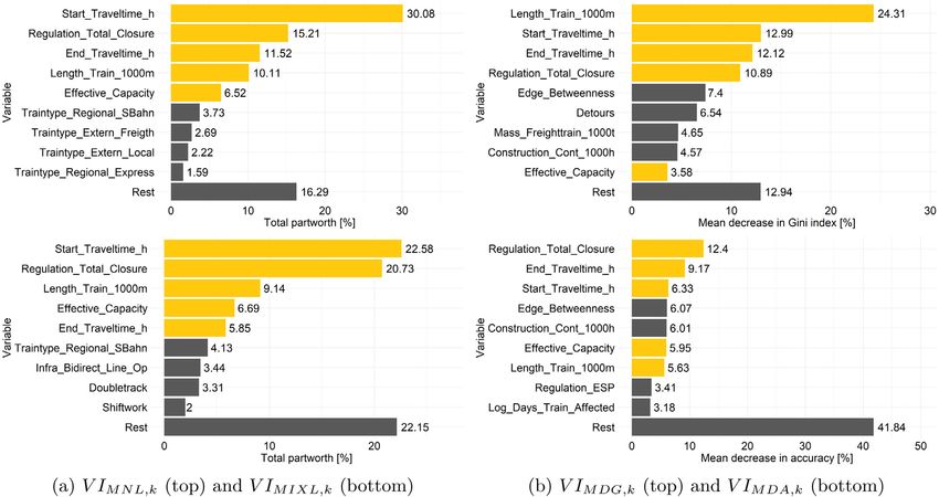
B. Schmid et al. Journal of Rail Transport Planning & Management 22 (2022) 100320

 Table 3
 Confusion matrix [economist method; in %] in the RF model for the 2021 (top) and 2022 (bottom) test datasets. Horizontal:
 Observed. Vertical: Predicted. In red: Problematic cases (3% or higher absolute mis-classification) where the model fails to predict
 correctly.
 2021 test dataset.
 KA: Pre. [%] KM: Pre. [%] KE: Pre. [%] U: Pre. [%] V: Pre. [%] Sum
 KA: Obs. 4.25 1.71 1.07 1.92 1.30 10.25
 KM: Obs. 0.83 7.63 1.30 1.98 1.96 13.70
 KE: Obs. 0.77 1.80 5.74 3.70 2.14 14.15
 U: Obs. 0.92 1.35 1.67 35.46 5.58 44.98
 V: Obs. 0.69 0.86 0.86 7.00 7.50 16.91
 Sum 7.46 13.35 10.64 50.06 18.48 100.00
 2022 test dataset.
 KA: Obs. 3.96 1.69 3.16 2.32 1.54 12.67
 KM: Obs. 0.91 6.12 2.86 2.14 1.16 13.19
 KE: Obs. 0.94 1.13 5.93 3.19 1.86 13.05
 U: Obs. 1.46 1.29 3.23 33.25 6.53 45.76
 V: Obs. 0.49 0.62 1.05 6.09 7.08 15.33
 Sum 7.76 10.85 16.23 46.99 18.17 100.00

 Table 4
 Computation time (effective CPU hours) overview.
 Observations Parameters Random draws CPU hours
 CONST 151,901 4 – 0.00
 MNL 151,901 160 – 10.47
 MIXL 151,901 166 100 12 326.10
 RF 151,901 – – 0.14
 RF (2021 dataset for training) 248,751 – – 0.24
 RF (2020 & 2021 dataset for training) 400,652 – – 0.43
 ANN 151,901 – – 2.58
 SVM 151,901 – – 3.94
 RFULL 151,901 103 – 1.35
 RFULL (2020 & 2021 dataset for training) 400,652 103 – 8.57
 RCOMP I (data compression ≈ 5×) 30,000 103 – 0.38
 RCOMP II (data compression ≈ 10×) 15,000 103 – 0.08
 RSIMP (data compression ≈ 10×) 15,000 79 – 0.05
 RBOX (data compression ≈ 10×) 15,000 89 – 0.44
 RMIXL (data compression ≈ 10×) 15,000 95 2000 352.30
 RRF 151,901 – – 0.13

in predicting the aggregated market shares than the MNL and MIXL models, although one of their main focuses is to reproduce
them (e.g. Ben-Akiva and Lerman, 1985; McFadden, 1986). The average market share prediction error for all five alternatives is
2.7% (2021) and 2.9% (2022) in the RF model, and 3.3% (2021) and 3.6% (2022) in the MIXL model, a similar result that has been
found in Zhao et al. (2020).
 Results indicate that the train route schedulers should be careful when making their final decisions based on the model
predictions. Specifically, if the model predicts e.g. a detour (U), one should keep in mind that delay (V) is the most common
mis-classification and that it may need more detailed considerations between these two alternatives. One reason may be due to
shortcomings in the data, such that if e.g. the capacity is reduced due to construction and one train is delayed and the other
is diverted, the choice which train receives which consequence might to some extent be arbitrary. Nevertheless, together with the
results presented in Section 4.3 and later in Section 4.5, this analysis can serve as a very useful tool in choosing the ‘‘best’’ alternative
in an informed way.

4.3. Variable importance (VI)

 Variable importance (VI) of attribute is calculated according to Section 3.5 for the discrete choice models using , , 
as well as for the best performing machine learning classifier, the RF model, using both metrics, , and , . Starting
with the MNL model, Fig. 4 shows that the top nine variables already account for 83.7% of the total utility partworth, with the top
five accounting for more than 66%. Given the modeling features of the different approaches, one may assume that from a behavioral
perspective, the MIXL would give the most accurate results, since it accounts for unobserved construction site heterogeneity — an
issue that has been shown to increase the model fit enormously. Nevertheless, the top nine VI in the MIXL are similar to the MNL
model, though a bit less pronounced (the top nine variables contain 77.8% of total utility partworth). Results clearly indicate that

 11

B. Schmid et al. Journal of Rail Transport Planning & Management 22 (2022) 100320

Fig. 4. Top nine variable importance (VI) of the discrete choice (MNL and MIXL; left) and Random Forest (RF; right) models. Orange bars: Same top attributes
according to all different modeling and VI calculation approaches (MNL, MIXL, RF MDG and RF MDA).

only a few among the full set of variables are actually important in explaining the behavior of train route schedulers, and that many
do not explain much; a good example of the Pareto principle.
 In both the MNL and MIXL model, the most important variable is Start_Traveltime_h that is mainly related to the very
strong and negative effect on KA as shown in Table A.3 and the relatively high mean value of that attribute as shown in
Table A.2. Regulation_Total_Closure is the second most important variable in both models. After that, both rankings include the
same variables End_Traveltime_h, Length_Train_1000m and Effective_Capacity but in slightly different order. The top six variable is
Traintype_Regional_SBahn and again is the same in both models. Then, while in the MNL model certain train types exhibit a higher
importance, construction site and infrastructure attributes play a more important role in the MIXL model. Importantly, however,
note that all train types taken together (since train type is a categorical variable and for estimation was split into dummy variables)
would – for all models and metrics – exhibit a relatively high importance ( = 14.5%; = 11.9%; = 7.3%;
 = 14.4%; the complete list of VI for all measures and variables is shown in the Appendix in Table A.5).
 The two VI metrics in the RF case – based on exactly the same model – show different rankings and relative importance values,
but there are again the same five top attributes in the top nine as in the discrete choice models. VI according to the MDG is most
comparable to the choice models, with the top nine attributes accounting for 87.1% of total VI. Notably, it shows a slightly lower
gradient, thus VI is more dispersed among the top nine. Length_Train_1000m now is the most important variable (24.3%), followed
by Start_Traveltime_h and End_Traveltime_h. The top nine include different attributes than in the choice models, with Edge_Betweenness
now becoming the fifth, Detours the sixth, Mass_Freighttrain_1000t the seventh and Construction_Cont_1000h the eighth most important
variable. The MDA finally shows a very distinct pattern in the sense that the top nine variables only account for 58.2% in total
VI; thus, variables classified as weak by the MDG as well as the discrete choice models exhibit a more important and uniformly
distributed importance. Also, Length_Train_1000m, which is the most important attribute according to MDG, now is on rank 7.20
 As discussed in Section 3.5, there may be a bias in VI in the RF model in favor of continuous variables for both the MDG
and MDA metric, indicated by the occurrence of Edge_Betweenness, Construction_Cont_1000h and others in the top nine variables,
which in the discrete choice models – assuming linear relationships – rank very low (e.g. in the MIXL: Edge_Betweenness on rank 18;
Construction_Cont_1000h on rank 24; see Appendix, Table A.5).
 Finally, a correlation analysis of the different VI measures according to Table A.5 shows that and are very
strongly related (+0.96), while and are not so much (+0.72). Furthermore, the correlation between and
 is also rather low (+0.68), while for and it is only slightly higher (+0.74).21 Results indicate that a critical

 20 For the sake of completeness, VI is also reported for the ANN model using 
 , , as shown in the Appendix, Fig. A.1 and Table A.5. It should be
noted that the VI pattern and ranking differs remarkably between the RF and discrete choice models. It is most comparable to the MDA given its uniformly
distributed VI and exhibits four top features that are also included in the MNL, MIXL and RF models. Interestingly, Regulation_Total_Closure is not part of the top
nine features, which – from a behavioral point of view – is rather questionable.
 21 
 exhibits the lowest correlations among all methods, which is highest with (+0.66).

 12