Deep Learning for Robust Super-resolution - HARVEST
←
→
Page content transcription
If your browser does not render page correctly, please read the page content below

Deep Learning for Robust
 Super-resolution

 A thesis submitted to the
 College of Graduate and Postdoctoral Studies
 in partial fulfillment of the requirements
 for the degree of Master of Science
 in the Department of Electrical and Computer Engineering
 University of Saskatchewan
 Saskatoon, Canada

 By
 Mahdiyar Molahasani Majdabadi

© Copyright Mahdiyar Molahasani Majdabadi, May 2021. All rights reserved. Unless
 otherwise noted, copyright of the material in this thesis belongs to the author.

Permission to Use

In presenting this thesis/dissertation in partial fulfillment of the requirements for a Post-
graduate degree from the University of Saskatchewan, I agree that the Libraries of this
University may make it freely available for inspection. I further agree that permission for
copying of this thesis/dissertation in any manner, in whole or in part, for scholarly purposes
may be granted by the professor or professors who supervised my thesis/dissertation work
or, in their absence, by the Head of the Department or the Dean of the College in which
my thesis work was done. It is understood that any copying or publication or use of this
thesis/dissertation or parts thereof for financial gain shall not be allowed without my writ-
ten permission. It is also understood that due recognition shall be given to me and to the
University of Saskatchewan in any scholarly use which may be made of any material in my
thesis/dissertation.

 Disclaimer

Reference in this thesis to any specific commercial products, process, or service by trade
name, trademark, manufacturer, or otherwise, does not constitute or imply its endorsement,
recommendation, or favoring by the University of Saskatchewan. The views and opinions of
the author expressed herein do not state or reflect those of the University of Saskatchewan,
and shall not be used for advertising or product endorsement purposes

 Request for permission to copy or to make any other use of material in this thesis in
whole or in part should be addressed to:

Head of the Department of Electrical and Computer Engineering
57 Campus Drive
University of Saskatchewan
Saskatoon, Saskatchewan, Canada
S7N 5A9

 i
OR
Dean
College of Graduate and Postdoctoral Studies
University of Saskatchewan
116 Thorvaldson Building, 110 Science Place
Saskatoon, Saskatchewan S7N 5C9 Canada

 ii
Abstract

 Super Resolution (SR) is a process in which a high-resolution counterpart of an image
is reconstructed from its low-resolution sample. Generative Adversarial Networks (GAN),
known for their ability of hyper-realistic image generation, demonstrate promising results in
performing SR task. High-scale SR, where the super-resolved image is notably larger than
low-resolution input, is a challenging but very beneficial task. By employing an SR model,
the data can be compressed, more details can be extracted from cheap sensors and cameras,
and the noise level will be reduced dramatically. As a result, the high-scale SR model
can contribute significantly to face-related tasks, such as identification, face detection, and
surveillance systems. Moreover, the resolution of medical scans will be notably increased.
So more details can be detected and the early-stage diagnosis will be possible for many
diseases such as cancer. Moreover, cheaper and more available scanning devices can be used
for accurate abnormality detection. As a result, more lives can be saved because of the
enhancement of the accuracy and the availability of scans.

 In this thesis, the first multi-scale gradient capsule GAN for SR is proposed. First,
this model is trained on CelebA dataset for face SR. The performance of the proposed
model is compared with state-of-the-art works and its supremacy in all similarity metrics
is demonstrated. A new perceptual similarity index is introduced as well and the proposed
architecture outperforms related works in this metric with a notable margin. A robustness
test is conducted and the drop in similarity metrics is investigated. As a result, the proposed
SR model is not only more accurate but also more robust than the state-of-the-art works.

 Since the proposed model is considered as a general SR system, it is also employed for
prostate MRI SR. Prostate cancer is a very common disease among adult men. One in seven
Canadian men is diagnosed with this cancer in their lifetime. SR can facilitate early diagnosis
and potentially save many lives. The proposed model is trained on the Prostate-Diagnosis
and PROSTATEx datasets. The proposed model outperformed SRGAN, the state-of-the-
art prostate SR model. A new task-specific similarity assessment is introduced as well. A
classifier is trained for severe cancer detection and the drop in the accuracy of this model

 iii
when dealing with super-resolved images is used for evaluating the ability of medical detail
reconstruction of the SR models. This proposed SR model is a step towards an efficient and
accurate general SR platform.

 iv

Acknowledgments

 I would like to thank my supervisor, Professor Seok-Bum Ko for his dedicated support
and guidance throughout my M.Sc program. Without his encouragement and assistance, this
dissertation would not have been possible. I also thank the following people who have helped
me undertake this research: My lab-mates, especially Arman Haghanifar for his innovative
ideas, my B.Sc. supervisor, Dr. B. Shokouhi for his support and encouragement, Dr. S.
Deivalakshmi and her team from the National Institute of Technology, Tiruchirappalli for her
help and support in taking this thesis to the next level, and my family, who have paved this
road for me with their endless support and patience. My sincere thanks to the Department
of Electrical and Computer Engineering, University of Saskatchewan.

 v
To the one who brought light and joy to my life.

 vi
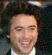
Table of Contents

Permission to Use i

Abstract iii

Acknowledgments v

Table of Contents vii

List of Abbreviations x

List of Tables xii

List of Figures xiii

1 Introduction 1

 1.1 Research problem and objectives . . . . . . . . . . . . . . . . . . . . . . . . 1

 1.2 Motivations . . . . . . . . . . . . . . . . . . . . . . . . . . . . . . . . . . . . 3

 1.2.1 Trends in Super-resolution . . . . . . . . . . . . . . . . . . . . . . . . 3

 1.2.2 Trends in Deep Learning Architectures . . . . . . . . . . . . . . . . . 6

 1.3 Super-resolution with Deep Learning . . . . . . . . . . . . . . . . . . . . . . 9

 1.4 Contributions of the Thesis . . . . . . . . . . . . . . . . . . . . . . . . . . . 10

 1.5 Publications and Submissions During M.Sc. Study . . . . . . . . . . . . . . . 11

 1.5.1 Published Journal . . . . . . . . . . . . . . . . . . . . . . . . . . . . . 11

 1.5.2 Published Conference . . . . . . . . . . . . . . . . . . . . . . . . . . . 12

 1.5.3 Preprints . . . . . . . . . . . . . . . . . . . . . . . . . . . . . . . . . 12

 1.6 Organization of the Thesis . . . . . . . . . . . . . . . . . . . . . . . . . . . . 12

 vii
2 Review of Super-resolution with Deep Learning 14

 2.1 CNN for Super-resolution . . . . . . . . . . . . . . . . . . . . . . . . . . . . 14

 2.2 GAN Based Super-resolution Models . . . . . . . . . . . . . . . . . . . . . . 16

 2.3 Face Super-resolution . . . . . . . . . . . . . . . . . . . . . . . . . . . . . . . 17

 2.4 MRI Image Super-resolution . . . . . . . . . . . . . . . . . . . . . . . . . . . 18

3 Capsule GAN for Robust Face Super-resolution 20

 3.1 Background . . . . . . . . . . . . . . . . . . . . . . . . . . . . . . . . . . . . 20

 3.1.1 Capsule Network . . . . . . . . . . . . . . . . . . . . . . . . . . . . . 20

 3.1.2 GAN . . . . . . . . . . . . . . . . . . . . . . . . . . . . . . . . . . . . 22

 3.2 MSG-CapsGAN . . . . . . . . . . . . . . . . . . . . . . . . . . . . . . . . . . 23

 3.3 Experimental Results and Discussions . . . . . . . . . . . . . . . . . . . . . . 27

 3.3.1 Dataset and Preprocessing . . . . . . . . . . . . . . . . . . . . . . . . 27

 3.3.2 Performance Metrics . . . . . . . . . . . . . . . . . . . . . . . . . . . 28

 3.3.3 Results . . . . . . . . . . . . . . . . . . . . . . . . . . . . . . . . . . . 30

 3.3.4 Comparison with State-of-the-Art . . . . . . . . . . . . . . . . . . . . 31

 3.3.5 Robustness Test . . . . . . . . . . . . . . . . . . . . . . . . . . . . . . 33

 3.4 Summary . . . . . . . . . . . . . . . . . . . . . . . . . . . . . . . . . . . . . 35

4 MRI Super-resolution 40

 4.1 Background . . . . . . . . . . . . . . . . . . . . . . . . . . . . . . . . . . . . 40

 4.1.1 Prostate Cancer . . . . . . . . . . . . . . . . . . . . . . . . . . . . . . 40

 4.1.2 MSG-GAN . . . . . . . . . . . . . . . . . . . . . . . . . . . . . . . . 42

 viii
4.2 Model Architecture . . . . . . . . . . . . . . . . . . . . . . . . . . . . . . . . 44

 4.3 Dataset and Preprocessing . . . . . . . . . . . . . . . . . . . . . . . . . . . . 46

 4.4 Results and discussions . . . . . . . . . . . . . . . . . . . . . . . . . . . . . . 49

 4.4.1 Similarity Assessment . . . . . . . . . . . . . . . . . . . . . . . . . . 49

 4.4.2 Experimental Results . . . . . . . . . . . . . . . . . . . . . . . . . . . 50

 4.5 Summary . . . . . . . . . . . . . . . . . . . . . . . . . . . . . . . . . . . . . 54

5 Conclusions and Future work 57

 5.1 Conclusions . . . . . . . . . . . . . . . . . . . . . . . . . . . . . . . . . . . . 57

 5.2 Future work . . . . . . . . . . . . . . . . . . . . . . . . . . . . . . . . . . . . 58

 ix
List of Abbreviations

AI Artifical Inteligence

CapsNet Capsule Network

CLAHE Contrast Limited Adaptive Histogram Equalization

CNN Convolutional Neural Network

DRE Digital Rectal Exam

FAN Face Alignment Network

FSIM Feature SIMilarity

GAN Generative Adverserial Network

HR High-Resolution

LOF List of Figures

LOT List of Tables

LR Low-Resolution

LSTM Long Short-Term Memory

MLP Multi-Layer Perceptron

MOS Mean Opinion Score

MPNR Mirror-Patch-based Neighbor Representation

MRF Markov random field

MS-SSIM Multi-Scale Structural SIMilarity

MSE Mean Square Error

MSG-CapsGAN Multi-Scale Gradient Capsule GAN

 x
PSA Prostate-Specific Antigen

PSNR Peak Signal-to-Noise Ratio

ReLU Rectified Linear Unit

ReLU Rectified linear unit

RNN Recurrent Neural Networks

RRDB Residual-in-Residual Dense Block

SR Super-Resolution

SSIM Structural SIMilarity

TSSA Task-Specific Similarity Assessment

VAE Variational Auto-Encoder

WL Windows Level

WW Windows Width

 xi
List of Tables

3.1 Experimental parameters and details. . . . . . . . . . . . . . . . . . . . . . . 30

3.2 The results . . . . . . . . . . . . . . . . . . . . . . . . . . . . . . . . . . . . 31

3.3 Comparison of the performance of different SR systems. . . . . . . . . . . . . 32

3.4 Comparison of the complexity of different face SR systems. . . . . . . . . . . 32

4.1 Comparison of the performance of different prostate SR models for 8× SR. . 51

4.2 Comparison of the performance of different prostate SR models for 4× SR. . 53

4.3 Comparison of the performance of different prostate SR models. . . . . . . . 53

4.4 Number of parameters in the proposed model and the state-of-the-art. . . . . 54

 xii
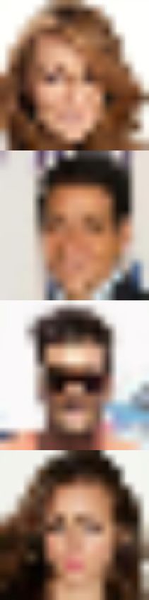
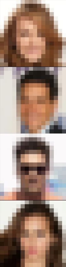
List of Figures

1.1 Super-resolution process with four steps: (1) ground-truth, (2) down-sampled
 image, (3) super-resolved sample, and (4) similarity metric. . . . . . . . . . . 4

1.2 Comparison between bicubic interpolation [1] and AI based SR. . . . . . . . 5

1.3 The architecture of (a) MLP, (b) CNN, (c) RNN, and (d) CapsNet. . . . . . 7

1.4 Some of the most common activation functions: (a) binary step, (b) identity,
 (c) Rectified Linear Unit (ReLU), (d) tanh, (e) sigmoid, and (f) swish. . . . 8

2.1 The PSNR of different convolutional SR models through time (from 2016 to
 2019) [2]. . . . . . . . . . . . . . . . . . . . . . . . . . . . . . . . . . . . . . . 15

2.2 Number of parameters of different convolutional SR models through time
 (from 2016 to 2019) [2]. . . . . . . . . . . . . . . . . . . . . . . . . . . . . . . 16

2.3 The architecture of FSRNet [3]. . . . . . . . . . . . . . . . . . . . . . . . . . 18

3.1 Two capsule layers . . . . . . . . . . . . . . . . . . . . . . . . . . . . . . . . 21

3.2 The architecture of a typical GAN. . . . . . . . . . . . . . . . . . . . . . . . 22

3.3 High level illustration of MSG-CapsGAN. . . . . . . . . . . . . . . . . . . . . 23

3.4 The architecture of up-sampling unit. . . . . . . . . . . . . . . . . . . . . . . 24

3.5 The architecture of the residual block. . . . . . . . . . . . . . . . . . . . . . 25

3.6 The value of hyperparameters through training. . . . . . . . . . . . . . . . . 26

3.7 High level illustration of the proposed VGG Residual network. . . . . . . . . 27

3.8 3 samples from CelebA aligned dataset. . . . . . . . . . . . . . . . . . . . . . 28

 xiii
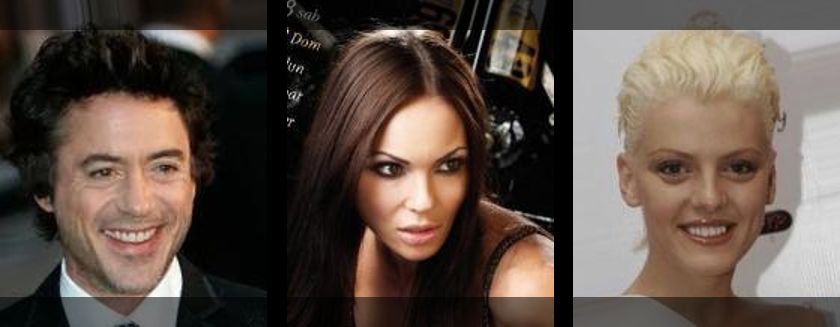
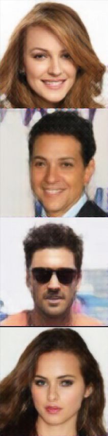
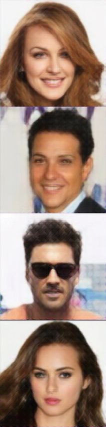
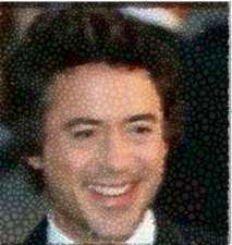
3.9 (a)16 × 16 input (b)Bilinear (c)Progressive [4], (d)Proposed Patch GAN,
 (e)Proposed VGG Residual, and (f)High resolution 128 × 128. . . . . . . . . 33

3.10 The transformation used in the robustness test. . . . . . . . . . . . . . . . . 34

3.11 The percentage of drop in (a) PSNR, (b) SSIM, (c) MS-SSIM, and (d) FSIM
 vs the rotation angle. . . . . . . . . . . . . . . . . . . . . . . . . . . . . . . . 35

4.1 The distribution of the new cancer cases in Canada in 2020 [5]. . . . . . . . . 41

4.2 Samples of ultrasound images of (a) healthy prostate [6], (b) prostate with
 cancer [6], and the MRI of (a) healthy prostate [7], (b) prostate with cancer [8]. 42

4.3 The architecture of progressive GAN. . . . . . . . . . . . . . . . . . . . . . . 43

4.4 The architecture of MSG-GAN. . . . . . . . . . . . . . . . . . . . . . . . . . 43

4.5 The architecture of CheXNet [9]. . . . . . . . . . . . . . . . . . . . . . . . . 45

4.6 The architecture of DenseNet-121 [9]. . . . . . . . . . . . . . . . . . . . . . . 45

4.7 The architecture of the model for prostate MRI SR. . . . . . . . . . . . . . . 46

4.8 The process of obtaining dataset. . . . . . . . . . . . . . . . . . . . . . . . . 47

4.9 Samples from the dataset (a)wide sagittal, (b)sagittal, (c)axial, and (d)low-
 quality axial. . . . . . . . . . . . . . . . . . . . . . . . . . . . . . . . . . . . 47

4.10 Sample image from the dataset (a) without CLAHE and (b) after applying
 CLAHE. . . . . . . . . . . . . . . . . . . . . . . . . . . . . . . . . . . . . . . 48

4.11 TSSA calculation for a SR model. . . . . . . . . . . . . . . . . . . . . . . . . 50

4.12 (a) Ground truth, SR out put of the proposed model with the scale of (b)
 8×, (c)4×, (d)2×, and (e)LR. . . . . . . . . . . . . . . . . . . . . . . . . . . 51

4.13 (a)Ground truth, (b)proposed model, (c)SRGAN, (d)bicubic, and (e)LR. . . 52

 xiv
1. Introduction

 Super-Resolution (SR) methods can increase the number of pixels and the quality of an
image. As a result, a small noisy blurry picture can become a clear large image. In this
thesis, a novel general SR system is proposed. The latest advancements and trends in deep
learning and SR is presented in this chapter, followed by a summary of contributions of this
thesis and the publications and submissions during the M.Sc. program.

1.1 Research problem and objectives

 SR is is an ill-posed problem. The reason is the fact that different High-Resolution (HR)
images can have the same Low-Resolution (LR) counterpart. If the differences between the
two images are small, then after down-sampling, the images will be identical. Hence, finding
the most accurate reconstructed HR image is extremely challenging and impossible in some
cases. Moreover, due to the lack of information in the LR input, filling the gaps in the
super-resolved image needs prior knowledge. For example, in a 16 × 16 image, there are
256 pixels. Each pixel is represented by 3 8-bit values. In total, this image carries 3840
bits of information. However, after ×8 SR, the reconstructed image will have 245760 bits of
information. So, based on the available data in the LR image and the domain-specific prior
knowledge of the model, the new 241920 bits should be determined.

 These two major problems make accurate SR a very challenging task. Another important
quality that should be present in the super-resolved image, other than the accuracy, is being
realistic. Some methods, such as interpolations, can provide relatively accurate images but
they look blurry and can easily be identified as fake images. Since the similarity of images
is usually compared based on the pixel values, the models are forced to generate outputs

 1
similar to the ground truth. However, two images with the same similarity (i.e. PSNR) can
have a different level of being realistic. So it is very important to consider this in designing
the model. The new pixel values should be determined in a way that the super-resolved
image not only be accurate but also look photo-realistic. Based on the mentioned problems,
it is very important to design a model which could generate accurate and visually pleasant
HR images from LR inputs.

 The latest advancements in the field of deep learning are employed in this thesis with a
creative approach to form a novel architecture that could answer the need for a powerful gen-
eral SR system. The performance of this system is analyzed to demonstrate its merits from
different perspectives. The main objective of the SR system is accuracy. The reconstructed
HR images should be loyal to ground truth. To evaluate this quality of the proposed system,
various metrics are used. Because of the lack of proper metrics for SR system performance
from a perspective of a deep learning model, a novel similarity metric is proposed. More-
over, to investigate the performance of the system in preserving medical details crucial for
accurate diagnosis, a new task-specific similarity assessment is introduced, as well.

 Another important objective of this work is to propose a general SR system that could
perform well in various domains. In the literature, many SR systems are proposed for specific
domains. These models can perform with a high performance only in one type of data. For
example, many SR systems are designed specifically for face SR. The reason behind this is
these models are developed based on a specific type of data architecture-wise. Moreover,
the domain-specific information is utilized as well. This domain-specific information can
be acquired in different ways such as labeled data and pre-trained feature extractors. For
example, in the face SR, the model can have access to the facial attribute labels like gender,
age, etc., or a classifier trained to find these labels can be embedded in the model and provide
this information. In this thesis, in order to develop a general SR model, no domain-specific
information or feature extraction model is used in the proposed architecture. So the model
could be trained on any type of data. Furthermore, the robustness of the model became one
of our highest priorities. Therefore, one of the newest deep learning models is used in our
model, and the performance of the proposed system while facing transformation attack is

 2
compared with the state-of-the-art works.

1.2 Motivations

 Since the introduction of the Generative Adversarial Network (GAN), generative Deep
Learning (DL) models flourish unprecedentedly. This new concept of training enables the
DL model to synthesize hyper-realistic images. As a result, a great opportunity has been
provided for the generative models to improve their performance significantly. One of the
most popular generative tasks is SR where the high-resolution counterpart of a low-quality
image is reconstructed. These powerful GAN-based models alongside another novel architec-
ture called capsule network to motivate us to propose a new capsule GAN model for image
SR. The proposed model can contribute to many face-related tasks and also can potentially
save lives by providing the radiologist with higher quality medical scans.

1.2.1 Trends in Super-resolution

 SR is a challenging ill-posed problem attempting to reconstructing the HR image from
its LR counterpart. LR image can be modeled as follows [2].

 xLR = (xHR ⊗ K) ↓s +n (1.1)

Where x is the image, K is a blurry filter, ↓s is image down-sampling operation, and n
is the additive noise. Fig. 1.1 illustrates a diagram of down-sampling, SR, and similarity
assessment.

 3
(3)

 Super-Resolution Model
 (4)

 Similarity Similarity
 Metric Assessment

 Down-
 Blur
 sampling +
 (2)
 (1)

 Noise

 Down-sampling Super-Resolution Similarity-Assessment

Figure 1.1: Super-resolution process with four steps: (1) ground-truth, (2) down-sampled
image, (3) super-resolved sample, and (4) similarity metric.

 In this thesis, the down-sampling block is implemented by an average function. A window
of pixels is selected and the average of the pixel values is calculated. This value creates a
pixel value in the LR image. This process is performed in each channel. Regarding the
noise, it should reflect the characteristics of the noise of the sensor that the SR is going to
implemented on its output. In this thesis, white Gaussian noise and salt and pepper noise are
added to the image. The super-resolution model and the similarity metrics will be explained
in the next chapter. Interpolation methods are very fast SR methods. These mathematical
non-learning algorithms perform well in low-scale SR. However, they suffer from low-quality
outputs and high computational cost when the SR scale increases. Bicubic interpolation and
Lanczos resampling are two popular examples of these algorithms [10, 11].

 More advanced and efficient SR methods are learning-based or so-called example-based
algorithms. Most of these methods are usually using machine learning so they could learn
from thousands of examples. In these approaches, an HR image is reconstructed by learning
a mapping between LR and HR images. Fig. 1.2 compares the interpolation methods and
Artificial Intelligent (AI) for SR.

 4
Bilinear interpolation
 128x128

 16x16 Based on the location
 and the pattern of pixels, Prior
 AI it should be a female knowledge
 dark eyes.

 128x128

 Figure 1.2: Comparison between bicubic interpolation [1] and AI based SR.

 The interpolation methods are mathematical approaches aiming at finding new pixel
values based on the neighbor values. However, AI-based models fill the gaps based on the
content and the prior knowledge of the system acquired from the learning process. Basic
machine learning algorithms has been widely used for SR, such as Markov random field
(MRF) [12], Neighbor embedding methods [13], sparse coding methods [14], and random
forest [15].

 Since the introduction of deep learning, it has been widely used for SR [16–23]. These
models achieved promising performance relying on their ability to learn high-level and com-
plex features due to their complexity. The number of trainable parameters in these models
varies from 20K to 43M [2]. More details on the deep learning architectures utilized in SR
is provided in sections 2.1 and 3.1.2.

 An important and challenging step in the SR task is image quality and similarity assess-
ment, as depicted in Fig. 1.1. Many attempts have been made to propose task-specific image
quality and/or similarity metrics. However, in most cases, Mean Square Error (MSE) or MSE
based metrics such as Peak Signal-to-Noise Ratio (PSNR) are the main quality assessment
tools. MSE has shown inadequate precision in reflecting the true quality of an image [2].
More recently, content-based metrics such as perceptual loss and Feature SIMilarity (FSIM)
have been proposed [24]. It is an absolute necessity to define clear task-specific assessments

 5
for the sake of fair comparison and optimization. In other words, having a metric that can
reflect the true quality or similarity of images can facilitate model comparison and set a true
goal for the machine learning model optimization. In order to peruse this goal, two novel
similarity metrics are introduced in this thesis in section.

1.2.2 Trends in Deep Learning Architectures

 Deep learning is a sub-category of machine learning. Unlike traditional learning-based
methods, no handcrafted features are utilized in deep learning models. The informative and
optimized features required for each task and dataset are established through the training
process. Due to the complexity of these models, they can combine basic features to create
higher-level features. Hence, all three steps of basic feature detection, hierarchical high-level
feature generation, and decision making are performed simultaneously in a single training
process [25].

 Since the introduction of the Multi-Layer Perceptron (MLP) algorithm in 1960 [26], Ar-
tificial Neural Network (ANN) has become more popular for deep learning implementation
because of two reasons, high capacity and hierarchical structure. In the 80’s, the backprop-
agation algorithm was introduced and utilized for training MLP [27]. The next huge leap
in the deep learning world was the introduction of Convolutional Neural Network (CNN) in
1989 [28]. Recurrent Neural Networks (RNN) were the next deep learning model proposed
in 1990. These models can show temporal dynamic behavior [29]. Capsule network (Cap-
sNet), is one of the latest advancements in deep learning, achieved the state-of-the-art result
on classification problems [30]. Unlike CNN, CapsNet can learn the geometric relationship
between features, hence, it is more robust. More details on CapsNet is presented in section
3.1.1. Fig. 1.3 compares the four mentioned types of deep learning layers.

 6
T

 T

 *
 *

 (a) (b)
 T
 *

 Dynamic Routing
 Dynamic Routing
 * *

 Dynamic Routing
 (c) * (d)

FigureFigure
 4.2: 1.3: The architecture
 Sample image fromof the
 (a) MLP, (b) (a)
 dataset CNN, (c) RNN,
 without and (d) and
 CLAHE CapsNet.
 (b) after
applying CLAHE
Dynamic Routing

 The blue neurons represent the input layer, the weights are in yellow and the orange
 neurons are the layer’s output. In MLPs, each neuron is connected to all neurons in the next
 layer, through a weight, called the synapse. Each neuron simply aggregated all weighted
 inputs and apply an activation function on it to form its output. The problem with MLPs
 is the high number of parameters. CNNs convolve several filters to the input tensor. Each
 filter represents a certain feature and it is trainable. The output of the convolution is a
 feature map on the input. The next convolutional layer combines the lower-level features
 extracted by the previous layer to detect high-level and more complex features. Each unit in
 a traditional RNN such as Long Short-Term Memory (LSTM), RNN has two inputs. First
 31
 is the input of time step T and the second is the output of the unit in time step T − 1.
 By connecting the output of each unit to its input, these units can benefit from short-term
 memory and it makes them the perfect choice for learning from time series or language-
 related tasks. CapsNet represents each feature with a vector. The values in the vector
 correspond to the geometrical pose of the feature and the length represents the probability

 7
of its presence. Then. each feature makes a prediction for each higher-level feature. Finally,
dynamic routing finds the agreement between the predictions and creates the final vector
corresponding to each high-level feature or class.

 As mentioned earlier, each neuron applies a non-linear function called activation to the
weighted inputs. Many activation functions have been used in DL models so far. Fig. 1.4
demonstrates some of the most common activation functions.

 (a) (b) (c)

 (d) (e) (f)

Figure 1.4: Some of the most common activation functions: (a) binary step, (b) identity, (c)
Rectified Linear Unit (ReLU), (d) tanh, (e) sigmoid, and (f) swish.

 The activation function is usually chosen based on its range of output and the architec-
ture. For example, if the labels in a classification task are 0 and 1, the sigmoid function can
be used. In the traditional LSTM, sigmoid and tanh are used and in CNNs, ReLU is one of
the first choices.

 In 2014, a new class of unsupervised deep learning models have been introduced [31].
By using the competitive learning paradigm, GANs have achieved unprecedented results in
hyper-realistic sample generation. In section 3.1.2, the architecture and applications of this
model are reviewed.

 8
1.3 Super-resolution with Deep Learning

 Face SR is a fast-growing field that aims to enhance the resolution of facial images. These
systems attempt to reconstruct High-Resolution (HR) face images from their Low-Resolution
(LR) counterparts accurately. Due to the importance of facial details on human perception,
it is vital to preserving these facial details [32]. Face hallucination has widespread and
crucial applications in various face-related systems such as face recognition, video surveillance
system, and image editing [33].

 To reconstruct HR images accurately, several challenges should be overcome. First, for
large-scale face SR, reconstructing an accurate HR image is an arduous task due to the lack
of information in the LR input. Second, it is required that the HR image not only possesses
similarity to the ground truth but also has a photo-realistic appearance and seems natural.
Finally, faces can appear in unlimited different poses. Hence, the facial SR system should
be pose-invariant to generalize for various situations.

 There are two categories of learning-based SR systems, local patch-based methods and
global methods. In the first category, the system is trained to reconstruct a patch of an
image at a time. Rajput and Arya propose a Mirror-Patch-based Neighbor Representation
(MPNR) system for face hallucination [34]. Their findings suggest that this system is capable
of filling missing parts in the face image, as well as super resolving noisy inputs. Several
studies have proposed global methods in order to implement a precise face SR system. In
these approaches, an HR image is reconstructed by learning a mapping between LR and
HR images [18, 35–37]. More recently, deep learning is widely used for facial SR. Yu et al.
propose a discriminative Generative Network to perform SR on aligned face images [38]. In
their next works [39, 40], multiple spatial transformations are utilized in order to enhance
the performance of the network. A cascade bi-network is introduced by Zhang et al. for
reconstructing HR unaligned faces from very low-resolution inputs [41]. These deep learning-
based methods improve the accuracy of face SR significantly. However, when the resolution
of the input is fairly low, the performance of these networks reduces due to the distortion in
the HR image.

 9
To overcome the image distortion issue, different approaches have been proposed. Gener-
ative Adversarial Networks (GAN) have shown promising results in image synthesis [31, 42].
Hence, it has been widely used for the SR task due to its natural-looking outputs. Ledig
et al. uses GAN for single image SR [43]. The perceptual loss function, which consists of
adversarial loss and content loss, is used for training the GAN for the SR task. Another ap-
proach is using prior knowledge and attribute domain information for SR, especially face SR.
This method is used for both Convolutional Neural Networks (CNN) and GANs. Kalarot
et al. propose CAGFace, a fully convolutional patch-based face SR system. A component
network is used to extract facial components and segment them. 4× face SR is performed
in their work. Lee et al. uses the information of the attribute domain as well as the image
domain to reconstruct facial details in the HR image precisely [33]. Cheng et al. use a face
shape estimation network for precise geometry estimation [3]. Kim et al. proposes a Face
Alignment Network (FAN) for landmark heat map extraction. A new facial attention loss is
applied for the training process based on their state-of-the-art FAN [4].

1.4 Contributions of the Thesis

 In [44], we have proposed a novel Multi-Scale Gradient Capsule GAN (MSG-CapsGAN)
for face SR to address the mentioned three challenges without using any attribute domain
information. Capsule GAN and Multi-Scale Gradient GAN have been used for the SR task for
the first time. The model has been trained on the CelebA dataset to increase the resolution
of images from 16 × 16 to 128 × 128. This network has surpassed the state-of-the-art SR
system in terms of PSNR.

 In the next step and in [24], we have improved and redesigned the MSG-CapsGAN to
enhance its performance and surpass previously introduced networks in all metrics. A robust
capsule GAN is proposed with a novel residual transfer-learning-based generator for multi-
scale face SR. The network is trained with an end-to-end training process without using any
attribute domain information.

 The proposed design has been optimized for prostate MRI SR. CheXNet has been embed-
ded in the model for feature extraction. A new task-specific approach for image similarity

 10
assessment is also introduced. The proposed model outperforms the state-of-the-art prostate
SR system.

 The contributions of this thesis are summarized as follows:

 1. We utilize Capsule GAN and Multi-scale GAN for the SR task for the first time.

 2. The proposed SR system surpassed the state-of-the-art systems in terms of PSNR,
 Structural SIMilarity (SSIM), Multi-Scale Structural SIMilarity (MS-SSIM), and Fea-
 ture SIMilarity (FSIM).

 3. The robustness of the network is evaluated and outperforms the state-of-the-art face
 SR system.

 4. The model is used for prostate SR and outperforms the state-of-the-art prostate SR
 system.

 5. A new task-specific metric for SR performance evaluation is introduced, called TSSA.

1.5 Publications and Submissions During M.Sc. Study

1.5.1 Published Journal

 1. Molahasani Majdabadi, Mahdiyar, and Seok-Bum Ko. ”Capsule GAN for robust face
 super resolution.” Multimedia Tools and Applications 79, no. 41 (2020): 31205-31218.
 DOI: 10.1007/s11042-020-09489-y

 A Major portion of this paper is included in Chapter 3: Capsule GAN for RobustFace
 SR

 2. Molahasani Majdabadi, Mahdiyar, Shahriar B. Shokouhi, and Seok-Bum Ko. ”Ef-
 ficient Hybrid CMOS/Memristor Implementation of Bidirectional Associative Mem-
 ory Using Passive Weight Array.” Microelectronics Journal 98 (2020): 104725. DOI:
 10.1016/j.mejo.2020.104725

 11
1.5.2 Published Conference

 1. Molahasani Majdabadi, Mahdiyar, and Seok-Bum Ko. ”Msg-capsgan: Multi-scale
 gradient capsule gan for face super resolution.” In 2020 International Conference on
 Electronics, Information, and Communication (ICEIC), pp. 1-3. IEEE, 2020. DOI:
 10.1109/ICEIC49074.2020.9051244

 A Major portion of this paper is included in Chapter 3: Capsule GAN for RobustFace
 SR

 2. Haghanifar, Arman, Mahdiyar Molahasani Majdabadi, and Seok-Bum Ko. ”Auto-
 mated Teeth Extraction from Dental Panoramic X-Ray Images using Genetic Algo-
 rithm.” In 2020 IEEE International Symposium on Circuits and Systems (ISCAS), pp.
 1-5. IEEE, 2020. DOI: 10.1109/ISCAS45731.2020.9180937

1.5.3 Preprints

 1. Haghanifar, Arman, Mahdiyar Molahasani Majdabadi, and Seokbum Ko. ”Covid-
 cxnet: Detecting covid-19 in frontal chest x-ray images using deep learning.” arXiv
 preprint arXiv:2006.13807 (2020).

 2. Haghanifar, Arman, Mahdiyar Molahasani Majdabadi, and Seok-Bum Ko. ”PaXNet:
 Dental Caries Detection in Panoramic X-ray using Ensemble Transfer Learning and
 Capsule Classifier.” arXiv preprint arXiv:2012.13666 (2020).

1.6 Organization of the Thesis

 The thesis is organized as follows:

 • Chapter 1: Introduction explains the motivation behind this research, followed by a
 description of SR with deep learning. Then, the contribution of this thesis is presented,
 and finally, the publications and submissions during the M.Sc. program are listed.

 • Chapter 2: Review of SR with Deep Learning provides a review on popular
 deep learning architectures for SR, including CNN and GAN. The latest advancements
 on face SR and MRI SR are also reviewed.

 12
• Chapter 3: Capsule GAN for Robust Face Super-resolution proposes a robust
 Multi-scale Gradient Capsule GAN for face SR. Then expand this model to enhance
 its performance. The performance of this model is evaluated and compared with the
 state-of-the-art works.

• Chapter 4: MRI Super-resolution explained the steps for applying the model
 proposed in Chapter 3 to a medical application. The architecture of prostate SR model
 is reviewed. Then, the dataset and the preprocessing pipeline is explained followed by
 the experimental results and comparison with related works.

• Chapter 5: Conclusions and Future work summarizes this thesis and discusses
 potential future works.

 13
2. Review of Super-resolution with Deep
 Learning

 In this chapter, a review of the Convolutional SR models are presented and the perfor-
mance of the most powerful CNN models are compared. Then, some of the best GAN-based
models for general SR are introduced. Face SR as a sub-domain of SR has been a trendy
topic in the last decade. These face SR models are explained in this chapter. Finally, SR in
medical imaging is discussed and the previous studies in this field are introduced.

2.1 CNN for Super-resolution

 SRCNN is a three-layer convolutional neural network utilized for SR. This shallow and
simple network is being trained with MSE loss function [45]. The first model using the normal
deconvolution layer is FSRCNN [46]. This model benefits from the deconvolution layer since
this layer reduces the computational complexity notably. An efficient sub-pixel convolutional
layer was proposed by Shi et al. which is called ESPCN [17]. Unlike ordinary deconvolution,
in the ESPCN layer, the dimension of the channel is increasing for the purpose of image
enlargement. As a result, a smaller kernel size is sufficient. Hence, the computational
complexity and training time can be reduced notably.

 It has been shown that deeper models with more layers can perform better in many tasks,
including SR [47]. VDSR is the first very deep model for SR [18]. This network uses the VGG
architecture and has 20 layers. This model is benefiting from multi-scale SR and residual
SR as well. Each image is super-resolved for many scales and the network is reconstructing
the high-frequency information and adds it to the bicubic interpolation of the LR image. To
reduce the number of parameters in VDSR, DRCN was introduced [19]. DRCN utilizes a

 14
recursive convolutional layer 16 times. To overcome the difficulty of training this model, a
multi-supervised learning strategy is implemented. In other words, the final result can be
considered as the result of the fusion of all 16 intermediate outputs. Since ResNet surpasses
VGG architecture in many tasks, it became an interesting choice for SR [48]. SRResNet was
proposed as the first ResNet for SR [43]. This model is using 16 residual units followed by
a batch normalization to stabilize the training process. Le et al. proposed EDSR which is
currently the state-of-the-art general SR model [21]. The main difference between EDSR
and SRResNet are first, the batch normalization layers were removed, second, the number
of output features were increased, and third, the weights for high-scale SR is initiated based
on ×2 SR weights.

 The performance of the aforementioned convolutional SR models alongside some other
famous SR models is compared in terms of PSNR in Fig. 2.1.

 33

 32.5

 32
 Chart Title
 33
 PSNR (dB)

 32.5
 31.5
 32
 31.5
 31
 31
 30.5
 30.5
 30
 29.5
 30
 29

Figure 2.1: The PSNR of different convolutional SR models through time (from 2016 to
2019) [2].

 Through time, the models are getting more complex and the PSNR of the outputs are
improving. Fig. 2.2 depicts the number of parameters in these models.

 15
100000

 Number of Parameters (Thousands) 10000 Chart Title
 33
 32.5
 1000
 32
 31.5
 100
 31
 30.5
 1030

 29.5

 129

Figure 2.2: Number of parameters of different convolutional SR models through time (from
2016 to 2019) [2].

 From 2016 to 2019, the number of parameters increases more than 750 times from 57k
to 43m. More powerful hardware for training and more efficient training algorithms make
this advancement possible.

2.2 GAN Based Super-resolution Models

 GAN-based SR systems are capable of learning to generate super-resolved images with
a similar distribution to the real samples. As a result, the outputs are more realistic and
visually pleasing in comparison with CNNs. SRGAN is the first GAN-based architecture
used for SR [43]. One of the main issues of the convolutional SR model is the dependency
of the loss on pixel values rather than the content. In order to tackle this problem, the
perceptual loss is utilized in SRGAN training. This loss function evaluates the similarity of
the content between the fake generated image and the ground truth. ESRGAN was proposed
to improve SRGAN architecture [49]. This model is benefiting from residual-in-residual dense
block (RRDB) in the architecture of its generator. The batch normalization layer has been
removed as well. A novel loss function, representing the texture similarity between generated

 16
images and real samples is used which improves the output quality.

2.3 Face Super-resolution

 Zhou et al. proposed the first CNN for face SR [50]. The features are extracted from
the LR image and combined through a fully connected layer to form the HR image. This
model uses 48 × 48 images in the output. TDAE, an auto-encoder-based architecture, was
proposed by Yu et al.. This model is trained to deal with noisy unaligned images [40].
TDAE is basically a decoder-encoder-decoder architecture. The image is up-sampled by the
decoder. Then the noise-free up-sampled image is passed to encoder-decoder architecture to
form a scale of ×8 super-resolved output. Grm et al. proposed CSRIP which is a cascaded
progressive CNN model [51]. A face recognition model is utilized alongside the model as well
to enhance the performance of CSRIP.

 To improve the visual quality of the outputs, the GAN-based models have been used
recently in the face SR models. URDGAN, proposed by Yu and Porikli, is a factor of 8 face
SR model trained with competitive learning paradigm [38]. Xu et al. improved the quality
of the outputs by proposing a new texture loss and using labeled data for the training [52].

 Various face SR models employ facial attribute domain information to enhance the visual
quality of the outputs, especially the facial details and expressions. This information can
be obtained from a facial feature extractor embedded in the GAN architecture. Yu et al.
proposed semantic clues which lead to its supremacy over previous works [53]. Li et al.
utilized two networks in order to embed the facial attributes extracted from the LR image
to the SR model [54]. Another approach for facial attribute information extraction is auto-
encoder. Variational Auto-Encoder (VAE), introduced by Liu et al., is used to extract
facial attributes from intermediate results [55]. The final output is generated by another
convolutional network benefiting from the provided information. Chen et al. used landmark
heat-map for training their CNN [3]. The architecture of their model is presented in Fig.
2.3.

 This facial prior enables their model to focus more on facial details by increasing the

 17
Fine SR Network

 Prior Estimation
 Network

 Fine SR
 Decoder
 Coarse SR Fine SR
 Network Encoder

 Figure 2.3: The architecture of FSRNet [3].

penalty for error in these areas. Another model that uses two CNNs is proposed by Wang
et al. [56]. First, ParsingNet obtains prior knowledge from the LR image. Then, FishSRNet
reconstructs the HR image benefiting from the provided information. Finally, Ge et al.,
employed teacher-student concept for face SR [57]. The teacher is trained on the complex
domain which is HR and then transfers its knowledge to the less complex model, the student.
So the student could imitate the behavior of the teacher on the LR domain.

2.4 MRI Image Super-resolution

 SR in medical imaging has been around for a while. The early works used image process-
ing algorithms for medical SR. Rousseau et al. employed anatomical inter-modality priors
obtained from a particular reference sample [58]. Peeters et al. interpolated slice-shifted
images in order to enhance signal to noise ratio [59]. Moreover, the effective slice thickness
was decreased as well.

 More recently, machine learning algorithms have become more popular for medical SR. A
2D convolutional network has been used by Yang et al. and Park et al. [60, 61]. 3D SR was
addressed by Chaudhari et al. and Chen et al. using 3D architectures [62,63]. These machine
learning approaches surpassed traditional image processing algorithms in both visual quality
and computational complexity.

 Among all machine learning algorithms, GAN performs the best for SR [64]. A GAN
using 3D convolutional layers is proposed by Li et al. for slice thickness reduction in MRI.

 18
SRGAN, as one of the first GAN models for SR, was utilized by Sood et al. for normal and
anisotropic SR in prostate MRI [65]. Their findings suggest that the visual quality of the
super-resolved images obtained by SRGAN is notably better than other approaches.

 19
3. Capsule GAN for Robust Face
 1
 Super-resolution

 Face hallucination is an emerging sub-field of SR which aims to reconstruct the HR
facial image given its LR counterpart. The task becomes more challenging when the LR
image is extremely small due to the image distortion in the super-resolved results. A vari-
ety of deep learning-based approaches have been introduced to address this issue by using
attribute domain information. However, a more complex dataset or even further networks
are required for training these models. In order to avoid these complexities and yet preserve
the precision in reconstructed output, a robust Multi-Scale Gradient capsule GAN for face
SR is proposed. A novel similarity metric called Feature SIMilarity (FSIM) is introduced as
well. The proposed network surpassed state-of-the-art face SR systems in all metrics and
demonstrates more robust performance while facing image transformations.

3.1 Background

 In this section, a brief review of capsule network architecture is presented. Afterward,
the concept of GAN and its applications are discussed.

3.1.1 Capsule Network

 Capsule Network consists of computational units called capsules. Each capsule is a group
of neurons nested together, which represent the substantiation parameters of a particular
feature by using a vector. This vector represents the pose parameters of the object. The

 1.Most of the parts in this chapter have been published in Majdabadi MM, Ko SB. ”Capsule GAN for
robust face super-resolution.” Multimedia Tools and Applications 79.41 (2020): 31205-31218.

 20
length of the vector corresponds to the probability of the presence of that particular feature.
Each vector is multiplied by a weight matrix to predict the vectors corresponding to each
higher-level feature. Then, dynamic routing evaluates the agreement of these predictions
and computes the final vector for each capsule in the second layer. Fig 3.1 indicates the
structure of two typical Capsule layers where m is the number of capsules in the first layer,
d1 is the size of each capsule in the first layer, n is the number of capsules in the second
layer, and d2 is the size of each capsule in the second layer.

 Predictions
 Weights
 First Capsule layer Second Capsule layer

 Dynamic Routing
 × (1 × ) × ( × × ) × ( × 1 × ) × (1 × )

 Figure 3.1: Two capsule layers

 Unlike CNN, CapsNet is capable of learning the hierarchy of the features and the geo-
metrical relationship between objects. This unique feature makes CapsNet a pose invariant
network. As a result, it has surpassed CNN in some classification tasks in terms of accuracy
and learning speed [66]. When a CNN is trained with a group of images in which a partic-
ular object always appears in a specific pose, the network is incapable of detecting the very
same object with a different pose. The reason is that the CNN has only learned to detect
the object only based on the presence of the combination of certain features and when the
pose of the object has been changed, the low-level features of the image such as edges differ
inevitably. Hence, this network is not robust to variations in the pose of the object. To
increase the robustness of the SR system, instead of using a bigger dataset or applying data
augmentation, CapsNet is utilized as the discriminator in the proposed SR network.

 21
3.1.2 GAN

 Similar to the animal learning behavior, GANs can learn through competition [67]. GAN
is using two deep learning models called generator and discriminator. The generator is
responsible for data generation and the discriminator is classifying samples into real and
fake classes. The discriminator is being trained to distinguish between the output of the
generator as synthesized samples and the real data and the generator’s goal is to fabricate a
data sample to deceive the discriminator. Fig. 3.2 depicts the architecture of a basic GAN.

 Discriminator training

 Sample
 Training dataset Real

 Generator training Real
 Discriminator Fake
 Sample
 Vector
 Input

 Fake

 Generator

 Figure 3.2: The architecture of a typical GAN.

Maximizing the accuracy of the fake and real image classification is the goal of the discrimi-
nator while the generator tries to minimize this accuracy by generating better fake samples.
It has been demonstrated that GAN is capable of imitating the distribution of the data [31].

 One of the challenges in training GANs is mode collapse. Mode collapse is a status of
the GAN when the model is not able to generalize. As a result of this error, the generator
is only producing the same or very similar outputs. Many solutions have been suggested
in order to overcome this issue, such as label smoothing. Label smoothing is a smart way
to prevent the discriminator from overfitting. By assigning 0.9 to one class and 0.1 to the
other class, the discriminator will face a penalty when it detects a fake or real sample with

 22
too much confidence (1 or 0). As a result, it can establish a more general understanding of
the real and fake samples. Noisy labels can improve the label smoothing process. A random
number in the neighborhood of 0.9 and 0.1 are assigned to real and fake classes, respectively.
As a result, the discriminator can’t overfit on the exact labels.

3.2 MSG-CapsGAN

 GAN has surpassed other deep learning approaches in many image-related applications,
especially SR task [53]. GAN mainly consists of two networks that are trained competitively,
Generator, and Discriminator. The high-level demonstration of the proposed network is
depicted in Fig. 3.3.

 128x128 128x128
 64x64
 32x32

 High resolution
 Up Sampling
 Up Sampling

 16x16
 Sampling
 Up

 input

 Generator
 down Sampling

 down Sampling

 High resolution
 Sampling
 down

 1 or 0 CapsNet

 32x32
 64x64
 Discriminator 128x128 128x128

 Figure 3.3: High level illustration of MSG-CapsGAN.

This architecture is called Multi-scale Gradient GAN (MSG-GAN), which is used for the
SR task for the first time in MSG-CapsGAN [44]. These intermediate connections can be
used as an alternative for progressive training, so great results have been acquired from this
architecture for synthesizing high-resolution images [68]. These promising results were the
primary motivation for using this idea for ×8 SR. The supremacy of this architecture over
other networks has been illustrated in our previous work [44].

 As far as the discriminator is concerned, in our work, CapsNet is utilized. CapsNet
benefits from some advantages over classic classifiers, especially, being pose-invariant [66].

 23
The input of the discriminator is either the super-resolved image or HR image, and its output
is 1 or 0 representing real or fake. First, the input image is down-sampled by using three
convolutional layers with the stride of 2 and the activation function of the leaky Rectified
Linear Unit (ReLU). Then the output is applied to a CapsNet with two layers. The primary
capsule layer has 32 capsules with 8 neurons in each capsule. The last layer contains 10
capsules with 16 neurons. Dynamic routing is performed for three iterations. Finally, the
output of CapsNet is connected to the output neuron with a fully connected layer. The

 Generator
activation function of and MSG-GAN
 the last layer is the sigmoid function, with the output in the range of

 High resolution
 Up Sampling

 Up Sampling
 Sampling
0 to 1.

 Up
 input

 The second network is the generator. The 16×16 pixel input is applied to the generator.
 Normalization

 Normalization
 Conv2D

 Conv2D

The image is up-sampled 3 times in order to reach 128×128 size. The architecture of the
 ReLU

 Batch

 Batch

 input +
up-sampling unit is depicted in Fig. 3.4.
 Residual

 Deconv
 Normalization
 Conv2D

 Conv2D
 Block
 ReLU

 Batch

 input +

 Figure 3.4: The architecture of up-sampling unit.

The first convolutional layer has 64 filters with a kernel size of 3×3. Then, ReLU is applied.
After the residual unit, a convolutional layer with the same parameters as the first Convo-
lutional layer is presented, and it is followed by a batch normalization layer. The output
is integrated with the output of the first convolutional layer. Finally, a deconvolution is
performed on the output results. The layer structure of the Residual Block is exhibited in
Fig 3.5.

All convolutional layers have 64 filters and the same padding. The input is added to the
output of the last layer to form the output of the residual block.

 By using 2RGB layers after intermediate connections, a multi-scale SR model can be
acquired. These layers are basically 3-filter convolutional layers, where each filter represents

 24
Generator and MSG-GAN

 Up Sampling
 Sampling
 Up
 input

 Normalization

 Normalization
 Conv2D

 Conv2D
 ReLU

 Batch

 Batch
 input +

 down Sampling
 Sampling
 down
 Figure 3.5: The architecture of the residual block. 16x16

one channel in the output tensor. So rather than only using these connections for passing

 Residual
the information between the generator and the discriminator layers, they can also be utilized

 Deconv
 Normalization
 Conv2D

 Conv2D
 Block
 ReLU

 Batch
for multi-scale training. + used for training the
 input Eq. 3.1 shows the perceptual loss function
generator.

where lSR is the training loss, S is a group of different scales which is {32, 64, 128}, liSR is
 SR
the content loss for each scale, and lGAN is the GAN loss. The content loss is computed as
follows:

 (fV GG19 (xi , 9) − fV GG19 (yi , 9))2
 liSR = (3.1)
 N

where fV GG19 (xi , 9) and fV GG19 (yi , 9) are the outputs of the ninth layer of VGG19 network
with the input of the generated image and the true image with the scale of i, respectively and
N is the number of elements in this feature vector. Both the HR image and super-resolved
image are passed to the VGG19 network and the similarity of the vector feature in the 9th
layer of the network is evaluated using Mean Square Error (MSE).

 In the next step of improving MSG-CapsGAN, the network has been forced to learn easier
steps first, inspired by the progressive training. Then, the task is gradually getting more
complex. In order to implement this training approach, the loss function has been modified
as follows:

 X
 lSR = ai × liSR + 3E(−3)lGen
 SR
 (3.2)
 i∈S

 25
The hyperparameter ai shows the state of the network in the training and controlling the contribution of each error to the final loss. These hyperparameters are adjusted according to the Fig 3.6. 1.0 0.8 Hyperparmeter value 0.6 0.4 0.2 a_32 a_64 0.0 a_128 0 10000 20000 30000 40000 50000 Epoch Figure 3.6: The value of hyperparameters through training. At the beginning, a32 , is equal to 1, and all other hyperparameters are equal to 0. Hence, the only content loss that matters is for the scale of 32. Then, the contribution of the a64 and a128 increases gradually. Studies demonstrate that using a matrix as a representation of being real or fake can improve the performance of the GAN notably. This network is called patch GAN [69]. Inspired by this idea, the output of the discriminator is redesigned. A fully connected layer with 4900 neurons is connected to the last capsule layer. Each value of each capsule is connected to all of the neurons through a weight. Then, the 4900 neurons are rearranged to 70 × 70 array of values in the range of 0 to 1, where 0 represents fake, and 1 represents real. In order to further reduce the artifacts in the output image, two approaches are taken. First, fully residual architecture is utilized. These types of networks are proven to be effective for image correction and SR [70]. Second, transfer learning can boost the performance of the proposed network since very informative features can be extracted using pre-trained models. Fig. 3.7 shows the diagram of the proposed architecture. 26
New generator architecture

 Concatenate 128x128 128x128
 16x16
 64x64 64x64

 sampling
 32x32

 Residual

 Up

 Up sampling
 16x16

 Up sampling
 Residual

 Residual

 Residual
 CNN
 128x128 VGG
 19
 Bicubic

 +
 64x64

 +
 32x32

 +

 32x32 64x64 128x128

 Figure 3.7: High level illustration of the proposed VGG Residual network.

The input image is up-sampled using the bicubic method, and then the network is recon-
structing the high-frequency details of the image. This high-frequency information is added
to the up-sampled image to form the output. It is also passed to VGG19 layers, and the fea-
ture map is extracted. Then, the extracted feature map is concatenated with the convolution
layers of the network so that the network could benefit from these features as well.

3.3 Experimental Results and Discussions

 The model is implemented using Tensor flow version 1 alongside with KERAS package.
The language used in this thesis is python. The codes for MSG-CapsGAN is publicly available
on GitHub 1 . The new layers implemented for this project are also published in the same
GitHub repository.

3.3.1 Dataset and Preprocessing

 To investigate the capability of the proposed network for facial SR task, aligned CelebA
dataset [71] is used in this study. CelebFaces Attributes Dataset (CelebA) is a large dataset
 1
 https://github.com/MahdiyarMM/MSG-CapsGAN

 27
of face images. The dataset is annotated with 40 binary labels such as mustache, eyeglasses,
smiling, etc. There are also 5 landmark locations provided. The images are collected form
the internet. Recently, the CelebA mask dataset is released as well. The dataset can be
accessed online 2 . This aligned dataset has been used so the robustness of the network could
be evaluated for different poses and angles of the faces later. The dataset is divided into
training and test-set with 162,770 and 19,867 images, respectively. Fig 3.8 exhibits some
samples from this dataset.

 Figure 3.8:
 Figure 3.8:3 3samples
 samples from CelebAaligned
 from CelebA aligned dataset
 dataset.

The size of works
 similar each image
 [36].is Finally,
 originally all × 178.
 218the As it is
 images areshown in Fig.
 resized to 3.8,
 12820× pixels
 128 as from
 HRthe
topimage
 and 20and
 pixels × 16the
 16 from as bottom
 LR images.
 of eachNo further
 image enhancements
 are cropped. or adjustments
 Hence, the final images are
 are applied to the dataset samples.
squares with a size of 178×178. Cropping the images reduces the background and enables us
to compare our results with similar works [4]. Finally, all the images are resized to 128 × 128
 3.3.2 Performance Metrics
as HR image and 16×16 as LR images. No further enhancements or adjustments are applied
 In order to evaluate the performance of the SR networks, three metrics are
to the dataset samples.
 mostly used:
3.3.21. PSNR:
 Performance Metrics
 Peak Signal to Noise Ratio
 2
 L three metrics are mostly used:
 In order to evaluate the performance of the SR networks,
 P SN R = 10 log10 ( ) (3.3)
 M SE
 1. PSNR: Peak
 where L Signal
 is thetomaximum
 Noise Ratiovalue in the image and MSE is the Mean
 Square Error of the super-resolved image.
 L2
 P SN R = 10 log10 ( ) (3.3)
 2. SSIM: Structural SIMilarity [65] M SE

 where L is the maximum value in 2µI µIˆand
 ˆ the image + kMSE
 1 isσthe
 I Iˆ + k2 Square Error of the
 Mean
 SSIM (I, I) = . (3.4)
 super-resolved image. µ2I + µ2Iˆ + k1 σI2 + σI2ˆ + k2
 2
 where µ is the mean, σ is the variance,
 σI Iˆ is the covarience between I
 http://mmlab.ie.cuhk.edu.hk/projects/CelebA.html
 ˆ and k1 and k2 are two constants.
 and I,
 28
 3. MS-SSIM: Multi-Scale Structural SIMilarity [66]
You can also read