Extent of Submerged Aquatic Vegetation - Albemarle-Pamlico ...
←
→
Page content transcription
If your browser does not render page correctly, please read the page content below
EXTENT OF SUBMERGED AQUATIC VEGETATION                                              METRIC REPORT
               HIGH-SALINITY ESTUARINE WATERS

Extent of Submerged Aquatic Vegetation
High-Salinity Estuarine Waters
Metric Report (REVISED*)

Don Field a, Jud Kenworthy a, Dean Carpenter b

INTRODUCTION

Why Is the Extent of Submerged Aquatic Vegetation Important Within
the Albemarle-Pamlico Estuarine System?

Underwater vascular plants are key components of aquatic ecosystems. They play multiple
roles in keeping Albemarle-Pamlico Estuarine System (APES) waters healthy by providing
habitat, food, and shelter for aquatic life; absorbing and recycling nutrients and filtering
sediment; and acting as a barometer of water quality.1 More commonly called “submerged
aquatic vegetation” (SAV), these plants enrich shallow aquatic environments around the world,
providing sanctuaries for mollusks, crustaceans, and finfish as well as sustenance for
waterfowl.2 SAV includes marine, estuarine, and riverine vascular plants that are rooted in
sediment3 and is one of five types of aquatic plants in APES waters, the others being floating
aquatic vegetation, emergent aquatic vegetation, micro- and macroalgae, and blue-greens
(cyanobacteria).4 Because SAV are rooted in anaerobic sediments, they need to produce a large
amount of oxygen to aerate the roots, and therefore have the highest light requirements of all
aquatic plants.5 SAV can become stressed by eutrophication and other environmental
conditions which impair water transparency and/or diminish the oxygen content of water and
sediments. The plant’s response to these factors enables them to be sensitive bio-indicators of
environmental health.6

While more than 500 species of SAV inhabit the world’s rivers, lakes, estuaries, and oceans7,
APES and its tidal tributaries are home to about 14 common species.8 High-salinity (10-30 ppt)
species, commonly referred to as seagrass include a temperate species, eelgrass (Zostera
marina), tropical species, shoalgrass (Halodule wrightii) and the eurytolerant species,
widgeongrass (Ruppia maritima), and the co-occurrence of these three species is unique to
North Carolina.9 Beds of SAV occur in North Carolina in subtidal water generally less than two
meters deep, and occasionally in intertidal areas of sheltered estuarine and riverine waters
where there is unconsolidated substrate (loose sediment), adequate light reaching the bottom,
and moderate to negligible current velocities or wave turbulence.10,11 SAV coverage ranges

* This version constitutes a revision of the metric report first posted on the APNEP website on February 18, 2021.
a NOAA National Centers for Coastal Ocean Science (Ret.), APNEP Science & Technical Advisory Committee
b
  APNEP
                                                                                                                1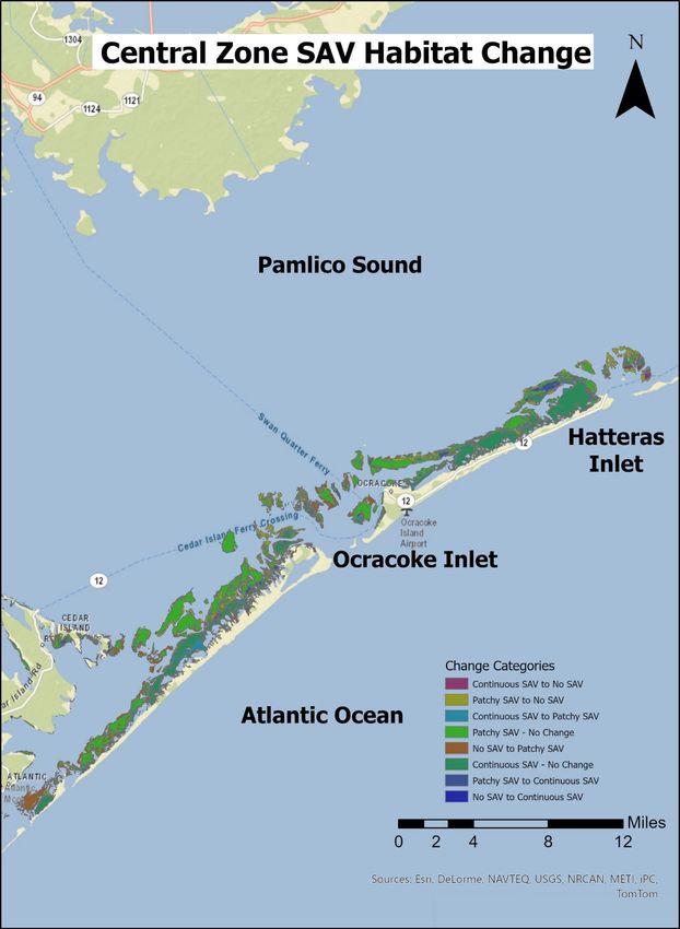
EXTENT OF SUBMERGED AQUATIC VEGETATION                                  METRIC REPORT:
             HIGH-SALINITY ESTUARINE WATERS                                           INTRODUCTION

from small, isolated patches less than a meter in diameter to continuous meadows covering
many acres (hectares or ha).

Because the distribution, abundance, and density of SAV varies seasonally and among years in
response to both environmental variability and human activity, large-scale SAV changes may
occur. The major threats to SAV habitat are channel dredging and water quality degradation
from excessive nutrient and sediment loading, as well as the emerging threat of accelerated sea
level rise, barrier island instability, increasing water temperatures and the expansion of shellfish
mariculture.12 The high value of this resource through its multiple ecosystem services makes it
essential that we have the ability to detect the onset of any dramatic declines or positive
responses from Albemarle-Pamlico National Estuary Partnership (APNEP)-led and other
protection and restoration activities via regular monitoring of this metric.13

What Does This Metric Report?

Within the APNEP region, true seagrass communities occur on the back-barrier shelves of the
Outer Banks between the U.S. Highway 64 Bridge that spans the sound between Roanoke Island
and the Outer Banks, south to Ocracoke Inlet, and on the Outer Banks and mainland shores of
Core, Back and Bogue Sounds. This metric reports the extent and location of those seagrass

                                                                                                2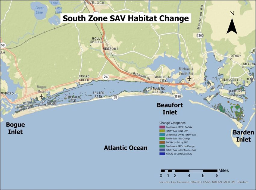
EXTENT OF SUBMERGED AQUATIC VEGETATION                               METRIC REPORT:
             HIGH-SALINITY ESTUARINE WATERS                                        INTRODUCTION

communities by spatial cover class (continuous, patchy, none) detected via aircraft during two
survey periods: 2006-2007 (Survey 1) and 2013 (Survey 2).

   •   Survey 1 (2006-2007)
          o May/June 2006: Aerial surveys of Bogue and Back Sounds between Barden Inlet
              and Bogue Inlet.
          o October 2007: Aerial surveys between Roanoke Island and Barden Inlet.
   •   Survey 2 (2013)
          o May 2013: Aerial surveys between Roanoke Island and Bogue Inlet.

During Survey 2, cloud cover issues rendered the acquired imagery for much of Core Sound
unsuitable for SAV Mapping (between Ophelia Inlet and Barden Inlet at Cape Lookout),
therefore extent and location measures for SAV in much of Core Sound are not included in this
report.

RESULTS
What Do the Data Show?

Spatial Trends
The areal extent of seagrass from Survey 1 was 100,843 acres (40,810 ha) while that from
Survey 2 was 95,157 acres (38,509 ha), a change of -5,686 acres (-2,301 ha) or -5.6% (Table 1).
Comparing continuous and patchy seagrass coverage between the two surveys showed a
15,773-acre (6,383-ha) loss of continuous seagrass, but a 10,087-acre (4,082-ha) gain of patchy
seagrass (Table 1). To investigate these changes in more detail, the data were subdivided in two
different ways: regionally and by categories of spatial cover class change. Regionally the data
were subdivided into three different zones: 1) the “North Zone” from the U.S. Highway 64
Bridge at Roanoke Island to Hatteras Inlet, 2) the “Central Zone” from Hatteras Inlet to Ophelia
Inlet and, 3) the “South Zone” from Barden’s Inlet near Cape Lookout to Bogue Inlet. The data
were also subdivided into eight spatial cover class change categories: continuous to none,
patchy to none, continuous to patchy, patchy both years of analysis, none to patchy,
continuous both years of analysis, patchy to continuous, and none to continuous.

Areal change data for the entire study area and regional zones are based on habitat polygons
that are generated from interpretation of digital multispectral imagery (see “Data
Manipulation” section of the Appendix), whereas the data for the categorial changes could not
be generated by comparing polygonal data from the two surveys and thus had to be rasterized.
Therefore, cross-comparisons between polygon-based (Tables 1, 2, 4 and 6) and raster-based
(Tables 3, 5, 7 and 8) calculations will generate areal inconsistencies.

                                                                                             3
EXTENT OF SUBMERGED AQUATIC VEGETATION METRIC REPORT:
HIGH-SALINITY ESTUARINE WATERS RESULTS
Table 1. Comparison of seagrass extent (acres, hectares in parentheses) in two spatial cover
classes and the total between the two surveys for the entire study area.
Spatial Cover Class Survey 1 Survey 2 Change % Change
Continuous 46,120 (18,664) 30,347 (12,281) -15,773 (-6,383) -34.2
Patchy 54,723 (22,146) 64,810 (26,228) 10,087 (4,082) 18.4
Total 100,843 (40,810) 95,157 (38,509) -5,686 (-2,301) -5.6
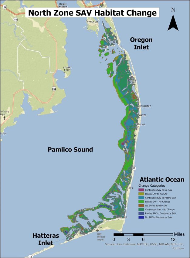
NORTH ZONE
Figure 1. Seagrass location and spatial cover classes (continuous and patchy) in the North Zone
during Survey 1 (2006-2007) and Survey 2 (2013).
The North Zone contained most of the seagrass mapped, with 70.3% of the seagrass in Survey 1
and 69.8% in Survey 2 (Figure 1). This zone also had the greatest overall seagrass habitat
change of the three zones with 4,416 acres (1,787 ha) lost (-6.2%) (Table 2). There was a 40.0%
loss (14,545 acres or 5,886 ha) of the continuous seagrass but a 29.4% gain (10,129 acres or
4,099 ha) of patchy seagrass.
4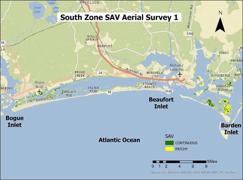
EXTENT OF SUBMERGED AQUATIC VEGETATION                                    METRIC REPORT:
             HIGH-SALINITY ESTUARINE WATERS                                                   RESULTS

Table 2. Comparison of seagrass extent (acres, hectares in parentheses) in two spatial cover
classes and the total extent between the two surveys for the North Zone, from the U.S. Highway
64 Bridge at Roanoke Island to Hatteras Inlet.

  Spatial Cover Class        Survey 1            Survey 2               Change          % Change
     Continuous           36,356 (14,713)     21,811 (8,827)        -14,545 (-5,886)      -40.0
        Patchy            34,505 (13,964)     44,634 (18,063)        10,129 (4,099)        29.4
         Total            70,861 (28,676)     66,445 (26,889)        -4,416 (1,787)        -6.2

The biggest component of the overall change in the North Zone was a conversion of 15,327
acres (6,203 ha) of continuous seagrass in Survey 1 to patchy seagrass in Survey 2 (Table 3,
Figure 2). The biggest habitat loss was 7,009 acres (2,836 ha) of patchy seagrass in Survey 1 that
was unvegetated in Survey 2. Most of that change was located at the outer western edges of
the patchy beds extending along the length of the North Zone.

Table 3. All possible categories of spatial cover class changes between the two mapping periods,
or classes remaining the same for the North Zone.

                    Spatial Cover Class Change Category         Acres (Hectares)
                  Continuous SAV to No SAV                              1,895 (767)
                  Patchy SAV to No SAV                                7,009 (2,836)
                  Continuous SAV to Patchy SAV                       15,327 (6,203)
                  Patchy SAV Both Years of Analysis                  24,310 (9,838)
                  No SAV to Patchy SAV                                4,462 (1,806)
                  Continuous SAV Both Years of Analysis              18,781 (7,600)
                  Patchy SAV to Continuous SAV                        2,646 (1,071)
                  No SAV to Continuous SAV                                 203 (82)

                                                                                                   5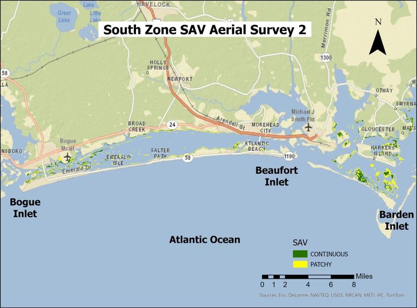
EXTENT OF SUBMERGED AQUATIC VEGETATION                               METRIC REPORT:
             HIGH-SALINITY ESTUARINE WATERS                                              RESULTS

Figure 2. Seagrass spatial cover class change categories in the North Zone from Survey 1 (2006-
2007) to Survey 2 (2013).

                                                                                             6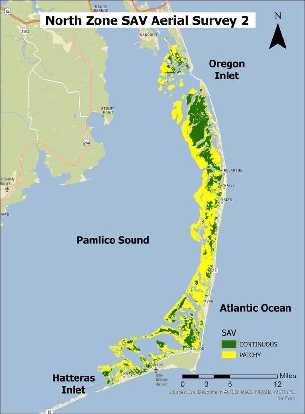
EXTENT OF SUBMERGED AQUATIC VEGETATION                                METRIC REPORT:
             HIGH-SALINITY ESTUARINE WATERS                                               RESULTS

CENTRAL ZONE

Figure 3. Seagrass location and spatial cover classes (continuous and patchy) in the Central Zone
during Survey 1 (2006-2007) and Survey 2 (2013).

The Central Zone contained the second-most seagrass area out of the three zones with 23.9%
of total seagrass area in Survey 1 and 24.7% in Survey 2 (Figure 3). Overall seagrass habitat
change in the Central Zone was a 655-acre (265-ha) loss (-2.7%). Like the Northern Zone, there
was a loss of continuous seagrass (896 acres or 363 ha, -11.7%) with a slight gain of patchy
seagrass (241 acres or 98 ha, 1.5%) (Table 4). While the overall increase in patchy seagrass was
relatively small, there was considerable conversion between patchy and continuous seagrass
and unvegetated sediment (Table 5, Figure 4). While there was a change of patchy seagrass to
unvegetated of 4,782 acres (1,935 ha), there was a change from unvegetated to patchy
seagrass of 4,386 acres (1,775 ha). Most of the conversions between unvegetated and patchy
seagrass occurred at the deep-water edge of beds or on shoals around Hatteras and Ocracoke
Inlets. There was also a conversion of 1,671 acres (676 ha) of continuous seagrass to patchy
seagrass.

                                                                                              7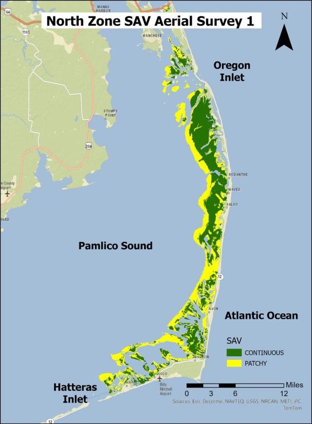
EXTENT OF SUBMERGED AQUATIC VEGETATION                                 METRIC REPORT:
             HIGH-SALINITY ESTUARINE WATERS                                                RESULTS

Table 4. Comparison of seagrass extent (acres, hectares in parentheses) in two spatial cover
classes between the two surveys for the Central Zone, from Hatteras Inlet to Ophelia Inlet.

  Spatial Cover Class       Survey 1             Survey 2              Change       % Change
     Continuous          7,672 (3,105)        6,776 (2,742)          -896 (-363)      -11.7
        Patchy           16,460 (6,661)       16,701 (6,759)          241 (98)          1.5
         Total           24,132 (9,766)       23,477 (9,501)         -655 (-265)       -2.7

Table 5. All possible categories of spatial cover class changes between the two mapping periods,
or classes remaining the same for the Central Zone.

                     Spatial Cover Class Change Category       Acres (Hectares)
                   Continuous SAV to No SAV                             401 (162)
                   Patchy SAV to No SAV                             4,782 (1,935)
                   Continuous SAV to Patchy SAV                       1,671 (676)
                   Patchy SAV Both Years of Analysis               10,186 (4,122)
                   No SAV to Patchy SAV                             4,386 (1,775)
                   Continuous SAV Both Years of Analysis            5,423 (2,195)
                   Patchy SAV to Continuous SAV                       1,112 (450)
                   No SAV to Continuous SAV                              150 (61)

                                                                                               8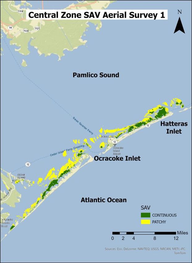
EXTENT OF SUBMERGED AQUATIC VEGETATION                               METRIC REPORT:
             HIGH-SALINITY ESTUARINE WATERS                                              RESULTS

Figure 4. Seagrass spatial cover class change categories in the Central Zone from Survey 1
(2006-2007) to Survey 2 (2013).

                                                                                             9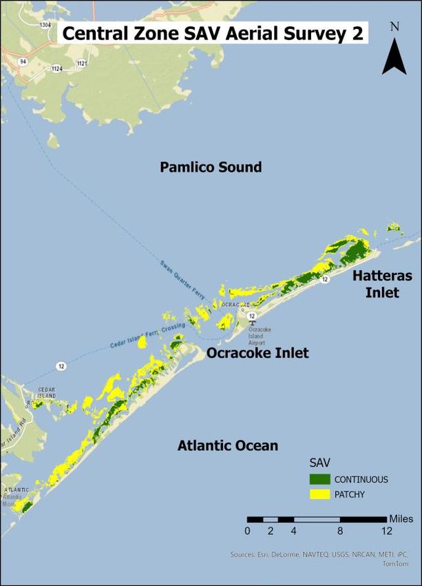
EXTENT OF SUBMERGED AQUATIC VEGETATION                               METRIC REPORT:
             HIGH-SALINITY ESTUARINE WATERS                                              RESULTS

SOUTH ZONE

Figure 5. Seagrass location and spatial cover classes (continuous and patchy) in the South Zone
during Survey 1 (2006-2007) and Survey 2 (2013).

                                                                                             10
EXTENT OF SUBMERGED AQUATIC VEGETATION METRIC REPORT:
HIGH-SALINITY ESTUARINE WATERS RESULTS
The South Zone contained the least seagrass of the three zones with 5.8% of the total seagrass
area in Survey 1 and 5.5% in Survey 2 (Figure 5). Overall seagrass habitat change within this
zone was a 615-acre (249-ha) loss (-10.5%). There was a loss of both continuous (332 acres or
134 ha, -15.9%) and patchy seagrass (283 acres or 115 ha, -7.5%) (Table 6). The largest
conversion was 1,218 acres (493 ha) of patchy seagrass to unvegetated (Table 7, Figure 6),
mostly at the deep-water edge of the beds.
Table 6. Comparison of seagrass extent (acres, hectares in parentheses) in two spatial cover
classes between the two surveys for the South Zone, from Barden Inlet at Cape Lookout to
Bogue Inlet.
Spatial Cover Class Survey 1 Survey 2 Change % Change
Continuous 2,092 (847) 1,760 (712) -332 (-134) -15.9
Patchy 3,758 (1,521) 3,475 (1,406) -283 (-115) -7.5
Total 5,850 (2,367) 5,235 (2,119) -615 (-249) -10.5
Table 7. All possible categories of spatial cover class changes between the two mapping periods,
or classes remaining the same for the South Zone.
Spatial Cover Class Change Category Acres (Hectares)
Continuous SAV to No SAV 88 (36)
Patchy SAV to No SAV 1,218 (493)
Continuous SAV to Patchy SAV 459 (186)
Patchy SAV Both Years of Analysis 1,706 (690)
No SAV to Patchy SAV 638 (258)
Continuous SAV Both Years of Analysis 1,277 (517)
Patchy SAV to Continuous SAV 216 (87)
No SAV to Continuous SAV 60 (24)
11EXTENT OF SUBMERGED AQUATIC VEGETATION METRIC REPORT:
HIGH-SALINITY ESTUARINE WATERS RESULTS
Figure 6. Seagrass spatial cover class change categories in the South Zone from Survey 1 (2006-
2007) to Survey 2 (2013).
12EXTENT OF SUBMERGED AQUATIC VEGETATION METRIC REPORT:
HIGH-SALINITY ESTUARINE WATERS DISCUSSION
DISCUSSION
What Is Not Shown by This Metric?
The data presented here cannot be compared to earlier SAV mapping efforts. While some pre-
2000 efforts to map SAV in the APNEP region have been performed, they are limited in scope
and used different techniques and classification schemes.
There are at least four older sources of mapping data under review for southern Core Sound
that may provide an opportunity to assess change in this important seagrass area, including
1981, 1985, 1988, and Fall 2007. Regarding more recent extent data, the entire geographic
range of high-salinity SAV in North Carolina was flown again in June 2019. Unfortunately, the
imagery from several areas was unsuitable for SAV mapping due to an assortment of wind,
turbidity, and haze issues. In response, APNEP sponsored additional flights for the geographic
range within the APNEP region in May and June 2020 and these data will be analyzed for the
next edition of this report.
Why is This Happening?
In some areas, such as natural inlets without jetties like Ophelia and Ocracoke Inlets, observed
seagrass change is primarily caused by the constant shift in shoal patterns.14 Another common
area of change is at the deep-water edge of patchy beds, particularly for the patchy beds that
run from Oregon Inlet to Cape Hatteras. In general, these are the deepest portions of the beds
and the areas of the meadows which are most exposed to wave energy originating from
northerly wind fetches. These areas would also be the most light-limited areas of the beds and
thus most vulnerable to changes in water clarity.
However, due to the natural variability in seagrass communities, change analysis based on only
two dates of imagery is by definition limited in scope. There are also no regularly scheduled
field monitoring or sentinel site activities for North Carolina’s seagrasses to provide the data
needed to help explain the correspondence between seagrass change and the factors that may
be responsible for the changes.15 Despite this, the mapping data (Tables 1, 2, 4, 6) and the
conversion data (Tables 3, 5, 7, 8) provide a compelling indication of the status and trends of
North Carolina’s seagrasses relative to global conditions, including other neighboring estuaries
on the Atlantic seaboard. However, based on the spatial cover class categorial change analysis
summary data in Table 8, all three zones (North, Central and South) of seagrass showed net
declines. Moreover, the decline in the South Zone (12.2% overall, 1.7% yr-1), where there is
relatively greater residential and commercial development and higher population densities, was
higher than in the other two zones. While it is difficult to determine with only two dates of
imagery, it appears the seagrass meadows in North Carolina may be in better condition than
many others throughout the world.16 The rates of decline in the North and Central Zones are
13EXTENT OF SUBMERGED AQUATIC VEGETATION METRIC REPORT:
HIGH-SALINITY ESTUARINE WATERS DISCUSSION
less than the global average for seagrasses since 1879 (1.5% yr-1), while the South Zone
exceeded the global average. However, all three regions were substantially lower than the
accelerating mean global declines reported since 1980 (5% yr-1).17 The relatively higher rate of
decline in the South Zone compared to the Central and North Zones may be indicative of
differential changes in environmental quality, especially nutrient and sediment loading
associated with shoreline development adjacent to the sounds and in the tributary watersheds.
Given the much larger land-to-water area ratio in Bogue and Back Sounds, as well as the
expansion of shellfish closure areas, seagrass in this region of the coast may be especially
vulnerable to the impairment of water quality and other anthropogenic activities.
Table 8. From-to calculations of the net change in seagrass extent (acres, hectares in
parentheses) in the three Albemarle-Pamlico Estuarine System zones for four spatial cover class
change categories. Annual change estimates for the North and Central Zones are based on 5.5
years and South Zone on 7.0 years between surveys. Spatial cover class conversion data for each
zone are based on Tables 3 (North), 5 (Central) and 7 (South).
CONVERSION ZONE
From To North Central South
None Patchy 4,462 (1,806) 4,386 (1,775) 638 (258)
None Continuous 203 (82) 150 (61) 60 (24)
Gain 4,665 (1,888) 4,536 (1,836) 698 (282)
Continuous None 1,895 (767) 401 (162) 88 (36)
Patchy None 7,009 (2,836) 4,782 (1,935) 1,218 (493)
Loss 8,904 (3,603) 5,183 (2,097) 1,306 (529)
Net Loss (Loss – Gain) 4,239 (1,715) 647 (262) 608 (246)
Total 69,968 (28,315) 23,575 (9,540) 4,964 (2,009)
% Change -6.1 -2.7 -12.2
% Change yr-1 -1.1 -0.5 -1.7
What Are the Implications for Management?
The data indicate that even with their differences in proximity to land development and
potential stressors, none of the three zones displayed increases in the extent of seagrass,
despite the availability of suitable habitat for expansion of the resource. The relatively higher
rate of decline in Back and Bogue Sounds (1.7% yr-1) in particular, should be on the radar of
those responsible for ensuring the sustainability of this resource. Given the global consensus
among scientists and resource managers that seagrasses are reliable indicators of water quality
and environmental health, yet severely threatened by impaired environmental quality, there is
an urgent need to continue to monitor this resource and integrate the status and trends of
14EXTENT OF SUBMERGED AQUATIC VEGETATION METRIC REPORT:
HIGH-SALINITY ESTUARINE WATERS DISCUSSION
seagrass with other collaborative environmental monitoring programs in North Carolina to
identify and manage the stressors responsible for the potential declines of seagrasses.
What are the Proposed Ultimate and Interim Targets for this Indicator?
Stakeholders within estuarine systems such as Tampa Bay, Florida derived ultimate targets with
reference to historical seagrass extent provided by aerial images from decades past. For the
limited APES waterbodies where historical aerial images of adequate quality exist to detect
seagrass extent, ultimate targets could be proposed in a similar manner. However, for the
majority of APES waterbodies where no such historical data archive exists, an ultimate target
may be derived from other ecological criteria, such as potential seagrass habitat. Potential
habitat models estimate spatial extent of SAV based on parameters such as water depth, water
quality, sediment type, and wind exposure.18
Pending the evaluation of other ecological criteria to facilitate the support of an ultimate
target, APNEP proposes a possible interim target based on Survey-1 estimates: attaining extent
for continuous and patchy spatial cover classes in all three zones, thus no loss since Survey 1
(2006-2007).
Acknowledgments
The authors thank Marygrace Rowe for her interpretation of the 2013 imagery and additional
work on the change detection analysis. We also thank APNEP staff members Tim Ellis, Kelsey
Ellis, and Patricia Murphey for their helpful comments on this manuscript. Anne Deaton of the
NC Division of Marine Fisheries has provided insight and support throughout this effort and
several members of her staff bore the brunt of the ground verification data collection.
The scientific results and conclusions, as well as any views or opinions expressed herein, are
those of the author(s) and do not necessarily reflect the views of NOAA or the Department of
Commerce.
Document Citation: Field, D., J. Kenworthy, and D. Carpenter. 2021. Metric Report: Extent of
Submerged Aquatic Vegetation, High-Salinity Estuarine Waters (REVISED). Albemarle-Pamlico
National Estuary Partnership. Raleigh, NC. 19 pp.
15EXTENT OF SUBMERGED AQUATIC VEGETATION METRIC REPORT:
HIGH-SALINITY ESTUARINE WATERS APPENDIX
APPENDIX
Data Description
All imagery was collected with Intergraph’s Z/I Digital Mapping Camera (DMC) (bands = red,
green, blue, near infrared). For the Survey-1 mapping effort, images along the mainland and
Outer Banks of Bogue Sound and Back Sound, and the mainland side of Core Sound north to
Atlantic, North Carolina were collected on May 31 and June 1, 2006. Aircraft height was 10,000
ft (3,048 m) for a final imagery product with 1 ft (0.3 m) pixel size. All other areas in the survey
area were collected on October 12, 14, and 15, 2007 with an aircraft height of 20,000 ft (6,096
m) for a final imagery product with 3.28 ft (1.0 m) pixel size.
For the Survey-2 mapping effort, all data were collected at an aircraft height of 10,000 ft (3,048
m) for a final imagery product with a 1 ft (0.3 m) pixel size. Images along the Outer Banks of
Pamlico Sound from Ocracoke Inlet to Manteo (north to Highway 64) were collected on May 30,
2013. Images along the mainland and Outer Banks of Bogue Sound and Back Sound were
collected on May 27, 2013.
Data Manipulation
The imagery was loaded into ArcGIS (Environmental Systems Research Institute) for manual on-
screen digitizing using procedures described by Rohmann and Monaco.19 Digitizing scale was
typically set to 1:1,500 except when larger homogenous areas required zooming out to a
greater extent that was usually accomplished at approximately 1:6,000. Habitat boundaries
were delineated around benthic habitat features (e.g., areas with visually discernable
differences in color and texture patterns). The scanned images were occasionally manipulated
in terms of brightness, contrast, and color balance to enhance interpretability of subtle features
and boundaries. This was extremely helpful, especially in deeper water where subtle
boundaries or problems caused by turbidity can made features difficult to detect. The
classification scheme consisted of three spatial cover classes: continuous seagrass, patchy
seagrass and unvegetated. Continuous seagrass was defined as areas covering 70% or greater
of the substrate that may contain unvegetated or sparsely vegetated areas that are smaller
than the minimum mapping unit (MMU = 0.2 ha in this study). Patchy seagrass was defined as
discontinuous communities covering more than 10% but less than 70% of the substrate. These
areas were diffuse and irregular consisting of isolated patches that are below the MMU. Areas
with less than 10% seagrass are considered beyond the level of detection of the imagery used
and thus were assigned the unvegetated or “No SAV” category.
Data Quality/Caveats
While the relative clarity and shallowness of high-salinity estuarine waters where seagrass
habitat exists in the APES allow a theoretical census of seagrass habitat via high-altitude aerial
surveys, there are places and conditions when the seagrass is invisible on the digital images
16EXTENT OF SUBMERGED AQUATIC VEGETATION METRIC REPORT:
HIGH-SALINITY ESTUARINE WATERS APPENDIX
regardless of the interpreters’ skills. For example, areas of high boat traffic or localized
thunderstorms can cause turbidity that can temporarily obscure seagrass beds.
There were also seasonal imagery acquisition differences that complicate the analyses. The
2007 imagery (1.0 m pixel resolution) for the North and Central Zones was acquired in
September/October, while all three zones in 2013 were acquired in May/June (0.3 m pixel
resolution). The South Zone was the only zone where imagery was acquired in the same season;
first in May 2006 (0.3 m resolution) and next in May 2013 (0.3 m resolution). The analyses are
confounded by the presence of two dominant seagrass species that have different seasonal
cycles of abundance. The temperate species, Zostera marina, reaches peak abundance in spring
and early summer, while the tropical species, Halodule wrightii, peaks in summer and early fall.
The ideal time period to capture both species in the imagery is in early summer, but due to the
poor atmospheric conditions it is very difficult to acquire imagery during the most ideal
signature period. Therefore, some of the changes observed in the North and Central Zones,
especially the conversions between continuous and patchy classes, could reflect the seasonal
transition in the relative abundance of the two species. To address this problem and minimize
the uncertainty in the change analysis above, a “net change” in seagrass extent was calculated
using only the conversions between no seagrass to each of the two spatial cover classes. Gains
were calculated by summing the conversions from no seagrass to patchy and continuous, while
losses were calculated using the sum of the conversions from the two classes to no seagrass.
The difference being the net change (Table 8).
Approximately 1,000 field points were visited in Survey 1 and 800 in Survey 2. The points were
randomly generated in GIS, based on areas where seagrass was previously mapped or in water
down to two meters in depth. Points were located in small craft with the aid of Differential
Global Positioning Systems (DGPS) or Wide Area Augmentation System (WASS). Areas were
identified visually from the boat (or wading in shallow waters) or with the aid of rakes where
the bottom could not be visualized. Field points from Survey 1 were used as training data in
some parts of the study area. Field points from Survey 2 did not become available in time to
inform the interpretation of that image data set. The field points, from both surveys, while
randomly selected were not used to perform accuracy assessments. It was determined that the
use of rakes, especially near the 2-m maximum depth of seagrass occurrence often missed
seagrass in obviously patchy areas, simply by raking between patches. It was also probable that
rakes sometimes picked up loose seagrass with root material, drifting along the bottom, giving
false positives for seagrass where none existed.
Data Availability
The data, in GIS format, can be downloaded here.
Data Gaps
Core Sound was not mapped. Due to cloud cover, imagery could not be acquired in 2013 or
2014. Therefore, Core Sound is not included in the change detection analysis.
17EXTENT OF SUBMERGED AQUATIC VEGETATION METRIC REPORT:
HIGH-SALINITY ESTUARINE WATERS APPENDIX
REFERENCES
1 Thayer, G.W., W.J. Kenworthy, and M.S. Fonseca. 1984. The Ecology of Eelgrass Meadows of
the Atlantic Coast: A Community Profile. FWS/OBS-84/02. U.S. Fish & Wildlife Service.
147 pp.
2 Bergstrom, P.W., R.F. Murphy, M.D. Naylor, R.C. Davis, and J.T. Reel. 2006. Underwater
grasses in Chesapeake Bay & Mid-Atlantic Coastal Waters: Guide to Identifying
Submerged Aquatic Vegetation. Maryland Sea Grant Publication Number UM-SG-PL-
2006-01. College Park, MD. 76 pp.
3 NCDEQ (North Carolina Department of Environmental Quality) 2016. North Carolina Coastal
Habitat Protection Plan Source Document. NC Division of Marine Fisheries, Morehead
City, NC. 475 pp.
4
Bergstrom et al. 2006.
5
NCDEQ 2016.
6 Biber, P.D., H.W. Paerl, C.L. Gallegos, and W.J. Kenworthy. 2004. Evaluating Indicators of
Seagrass Stress to Light. Pages 193-209 in S.A. Bortone, ed. Estuarine Indicators. CRC
Press, Boca Raton, FL.
7
Bergstrom et al. 2006.
8
NCDEQ 2016.
9
NCDEQ 2016.
10
Thayer et al. 1984.
11 Ferguson R.L., and L.L. Wood. 1994. Rooted Vascular Aquatic Beds in the Albemarle-Pamlico
System. Albemarle-Pamlico Estuarine Study Project 94-02. NOAA, National Marine
Fisheries Service, Beaufort Laboratory, Beaufort, NC. 103 pp.
12
NCDEQ 2016.
13 Carpenter, D.E., and L. Dubbs (Eds.). 2012. 2012 Albemarle-Pamlico Ecosystem Assessment.
Albemarle-Pamlico National Estuary Partnership, Raleigh, NC. 263 pp.
18EXTENT OF SUBMERGED AQUATIC VEGETATION METRIC REPORT:
HIGH-SALINITY ESTUARINE WATERS APPENDIX
14 Cunha, A.H., and R.P. Santos. 2009. The use of fractal geometry to determine the impact of
inlet migration on the dynamics of seagrass landscape. Estuarine, Coastal and Shelf
Science 84: 584-590.
15 Neckles, H.A., B.S. Kopp, B.J. Peterson, P.S. Pooler. 2011. Integrating scales of seagrass
monitoring to meet conservation needs. Estuaries and Coasts 35: 23-46.
16
Waycott, M., C.M. Duarte, T.J.B. Carruthers, R.J. Orth, W.C. Dennison, S. Olyarnik, A.
Calladine, J.W. Fourqurean, K.L. Heck, Jr., A.R. Hughes, G.A. Kendrick, W.J. Kenworthy,
F.T. Short, and S.L. Williams. 2009. Accelerating loss of seagrasses across the globe
threatens coastal ecosystems. Proceedings of the National Academy of Sciences
106(30): 12377-12381.
17
Waycott et al. 2009.
18 Koch, E.W. 2001. Beyond light: Physical, geological, and geochemical parameters as possible
submersed aquatic vegetation habitat requirements. Estuaries 24: 1–17.
19 Rohmann, S.O., and M.E. Monaco. 2005. Mapping Southern Florida’s Shallow-water Coral
Ecosystems: An Implementation Plan. Technical Memorandum NOS NCCOS 19.
NOAA/NOS/NCCOS/CCMA, Silver Spring, MD. 45 pp.
19You can also read