ENSEMBLE OF SIMPLE RESNETS WITH VARIOUS MEL-SPECTRUM TIME-FREQUENCY RESOLUTIONS FOR ACOUSTIC SCENE CLASSIFICATIONS
←
→
Page content transcription
If your browser does not render page correctly, please read the page content below

Detection and Classification of Acoustic Scenes and Events 2021                                                                        Challenge

ENSEMBLE OF SIMPLE RESNETS WITH VARIOUS MEL-SPECTRUM TIME-FREQUENCY
           RESOLUTIONS FOR ACOUSTIC SCENE CLASSIFICATIONS
                                                                 Technical Report

                                         Reiko Sugahara , Masatoshi Osawa , Ryo Sato

                                                      RION CO., LTD.
                                    3-20-41 Higashimotomachi, Kokubunji, Tokyo, Japan
                                        {r-sugahara, m-osawa, sato.ryou}@rion.co.jp

                            ABSTRACT
This technical report describes procedure for Task 1A in DCASE
2021[1][2]. Our method adopts ResNet-based models with a mel
spectrogram as input. The accuracy was improved by the ensemble
of ResNet-based simple models with various mel-spectrum time-
frequency resolution. Data augmentations such as mixup, SpecAug-
ment, time-shifting, and spectrum modulate were applied to pre-
vent overfitting. The size of the model was reduced by quantization
and pruning. Accordingly, the accuracy of our system was achived
70.1% with 95 KB for the development set.
   Index Terms— acoustic scene classification, ResNet, data aug-
mentation, ensemble, pruning

                       1. INTRODUCTION

Task1 SubtaskA (Task 1A) attempts to realize an acoustic scene
classification that is robust to multiple devices and has a limited
                                                                           Figure 1: Log-mel power as input; each sizes are 10 × 1996 (a), 20
model size. The development dataset comprises ten cities recorded
                                                                           × 998 (b), 65 × 250 (c), 120 × 125 (d), and 240 × 72 (e).
by nine devices. In addition, we analyze ten types of scenes. Be-
cause five new devices were added to the test data, it is necessary to
create a system that is robust to the differences between the devices.
The task also targets low complexity solutions for the classification       ensemble of models that specialize in different acoustic features.
problem in terms of model size. The data adopted must be 128 KB            We prepared five types of inputs as shown in Figure 1.
or less. The dataset for this task is TAU Audio-Visual Urban Scenes
2020[3], with a 44.1 kHz sampling rate and 24-bit resolution.              2.2. Network Architecture
     In this report, we first explain the method for the preprocessed
signal. We adopt log-mel power as input. Input sizes are prepared          ResNet[4] is a type of neural network known for its high perfor-
with various resolutions in the time and frequency for ensemble            mance, which has deep layers and inputs to some layers passed di-
learning (Section 2.1). Subsequently, we describe network archi-           rectly or as shortcuts to other layers. However, the base ResNet is a
tecture, which is based on ResNet and has a model size of 67.7             very large model and unsuitable for Task 1A; hence we use a simple
KB before compression. Three models with different inputs are              ResNet with fewer layers as shown in Figure 2.
prepared and ensemble learning is executed (Section 2.2). After in-             An ensemble is a fusion of different independently trained mod-
troducing data augmentations (Section 3) and model size reduction          els, which is known for its significant contribution to the improve-
(Section 4) , we provide some experimental results (Section 5) and         ment of accuracy. Therefore our network is architected by an en-
conclude the report (Section 6).                                           semble of models with different inputs. Using classified outputs of
                                                                           each ResNet-based model as input, we designed a fully connected
                                                                           model, as shown in Figure 3.
                    2. PROPOSED SYSTEMS

2.1. Audio Signal Preprocessing                                                              3. DATA AUGMENTATION
We adopt log-mel power as input for the ResNet-based model. The
                                                                           To prevent overfitting and accommodate device sources in the test
data set is mono and the common sampling rate is 44.1 kHz. We
                                                                           data, we adopt several data augmentation strategies. All strategies
attempted to improve the accuracy via ensemble learning using sev-
                                                                           do not generate extra training data.
eral models with different feature values. Input sizes are prepared
with various resolutions in the time and frequency, which is for an         • mixup[5]: Mixup is the process of mixing two sound sources
Detection and Classification of Acoustic Scenes and Events 2021                                                                  Challenge

                                                                          Figure 3: Example of a diagram with experimental results.

                                                                      4.1. Pruning
                                                                      Pruning is one of the methods for compressing the model size by
                                                                      changing unimportant weights to zero. The pruning method, which
                                                                      we applied was provided by Tensorflow Lite[8]. To maintain the
                                                                      classification accuracy of the original model, as much as possible,
                                                                      we set the final sparsity to 75%.

                                                                      4.2. Quantization

                 Figure 2: simple ResNet structure.                   As an alternative method for compressing the model size, we ap-
                                                                      plied post-trainingquantization provided by Tensorflow lite to our
                                                                      model. The weights of the original model are float32. By quantiz-
                                                                      ing them to int8, the size of the model can be compressed to ap-
   in an arbitrary proportion. Here we set α = 1.3, which is a        proximately 1/4 of its original size.
   parameter of β-distribution.
 • SpecAugment[6]: SpecAugment involves warping the fea-                                        5. RESULTS
   tures, masking blocks of frequency channels, and masking
   blocks of time steps. However, in our system, masking blocks       The dataset of TAU Urban Acoustic Scenes 2020 Mobile Develop-
   of frequency channels is solely applied. The masking rate is       ment dataset, it contains three real devices (A, B, C) and six sim-
   limited from 0% to 50%.                                            ulated devices (S1–S6) . Some devices (S4, S5, S6) are solely in-
                                                                      cluded in the test subset. We report the performance of our system
 • time-shifting: An index is determined randomly from the time
                                                                      compared to the baseline on the development set. The systems will
   axis, and the data is shifted from there.
                                                                      be ranked by macro-average multiclass cross-entropy (Log loss)
 • spectrum modulate: The above three methods are well-known          (average of the class-wise log loss).
   and conventional methods. To further improve robustness for            Table 1 presents the results of our systems and the baseline in
   unknown devices, we took original strategies based on a previ-     each device. The system 1, 2 and 4 are the ensemble of five models
   ous study[7]. Most of the provided datasets are recorded with      and the system 3 is the ensemble of three models. We adopt the
   device A. Therefore, we generated 3747 kinds of characteris-       weighted score average for the system 1 and 3, the score average for
   tics that can simulate devices other than A, which are generated   the system 2 and the weighted score average by the dance layer for
   by data obtained with device (B or C or S1 or S2 or S3) - A in     the system 4 as the decision making method. Compared with the
   log-mel power. By introducing the characteristics randomly for     DCASE 2021 task1A baseline system, our network structures are
   each batch, we aimed to cover the characteristics of the devices   improved by approximately 20%. The models worked each devices
   that were not in the original data set.                            evenly, without being weak in any specific device. From Figure 4,
                                                                      we can observe that the highest accuracy among all the classes is of
                                                                      the park at 96%.

                  4. MODEL COMPRESSION                                                       6. CONCLUSION

                                                                      In this technical report, we described a system for acoustic scene
In the DCASE CHALLENGE 2021 Task1A, the model complex-                classification Task 1A of DCASE challenge 2021. The network
ity limit is set to 128 KB for non-zero parameters. To compress       architecture is an ensemble of ResNet-based simple models with
our model size, we applied pruning and quantization to the model,     various mel-spectrum time-frequency resolutions. During training,
which is trained with float32.                                         data augmentation was applied to prevent overfitting and improve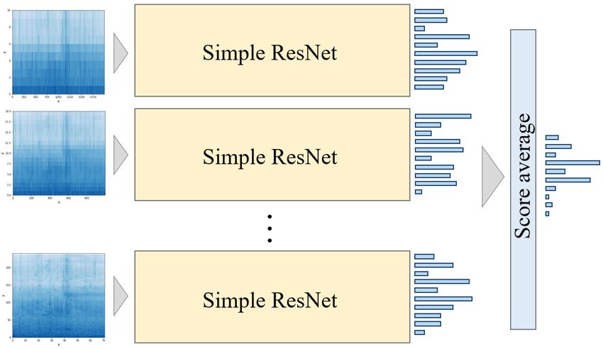
Detection and Classification of Acoustic Scenes and Events 2021                                                                      Challenge

                                         Table 1: Log loss on the development dataset for each systems.

                                                                               tion for multi-device audio: analysis of dcase 2021 challenge
                                                                               systems. 2021. arXiv:2105.13734.
                                                                           [3] Toni Heittola, Annamaria Mesaros, and Tuomas Virtanen.
                                                                               Acoustic scene classification in dcase 2020 challenge: gener-
                                                                               alization across devices and low complexity solutions. In Pro-
                                                                               ceedings of the Detection and Classification of Acoustic Scenes
                                                                               and Events 2020 Workshop (DCASE2020). 2020. Submitted.
                                                                               URL: https://arxiv.org/abs/2005.14623.
                                                                           [4] K. He, X. Zhang, S. Ren, J. Sun, Deep Residual Learning for
                                                                               Image Recognition, arXiv preprint arXiv:1512.03385, 2015.
                                                                           [5] H. Zhang, M. Cisse, Y. N. Dauphin, and D. Lopez-Paz,
                                                                                mixup: Beyond Empirical Risk Minimization, arXiv preprint
                                                                               arXiv:1710.09412, 2017.
                                                                           [6] D. S. Park, W. Chan, Y. Zhang, C. Chiu, B. Zoph, E. D.
                                                                               Cubuk, Q. V. Le SpecAugment: A Simple Data Augmentation
                                                                               Method for Automatic Speech Recognition , arXiv preprint
                                                                               arXiv:1904.08779, 2019.
                                                                           [7] M. Kosmider, Spectrum Correction: Acoustic Scene Classifi-
                                                                               cation with Mismatched Recording Devices, INTERSPEECH,
                                                                               pp. 4641–4645, Jan. 2020.
                                                                           [8] https://www.tensorflow.org/lite/performance/post training quant

 Figure 4: Confusion matrix for the validation data of system 1.

robustness to multiple devices. This allowed our proposal model to
perform better than the baseline.

                         7. REFERENCES

[1] http://dcase.community/challenge2021/index
[2] Irene Martı́n-Morató, Toni Heittola, Annamaria Mesaros, and
    Tuomas Virtanen. Low-complexity acoustic scene classifica-
You can also read