Dynamical study of Lyapunov exponents for Hide's coupled dynamo model
←
→
Page content transcription
If your browser does not render page correctly, please read the page content below
Demonstratio Mathematica 2021; 54: 189–195
Research Article
Teflah Alresheedi and Ali Allahem*
Dynamical study of Lyapunov exponents for
Hide's coupled dynamo model
https://doi.org/10.1515/dema-2021-0023
received March 11, 2021; accepted May 29, 2021
Abstract: In this paper, we introduced the Lyapunov exponents (LEs) as a significant tool that is used to
study the numerical solution behavior of the dynamical systems. Moreover, Hide’s coupled dynamo model
presents a valuable dynamical study. We simulate the convergence of the LEs of the model in three cases
by means of periodic flow, regular flow, and chaos flow. In addition, we compared these cases in logic
connections and proved them in a mathematical way.
Keywords: Lyapunov exponents, dynamical system, dynamo model, periodic flow, chaotic flow, regular flow
MSC 2020: 00A05, 11S82, 15A06, 15A60, 30C30
1 Introduction
The convergence or divergence average of exponential rates of nearby trajectories in the dynamical system
phase space is given by the Lyapunov exponents (LEs) [1]. It is named after Aleksandr Lyapunov who has
developed many major methods in 1899, which can be used to state the set of stability of the ordinary
differential equations (ODEs). There are two types of LEs. First, when the LEs are positive, the average
exponential of two nearby trajectories is diverge. Second, when the LEs are negative, the average exponential
of two close trajectories is converge [2]. Recently, the Lyapunov characteristic exponent (LCE) becomes a hot
research topic, which can be used to characterize the dynamical systems quantitatively and their stochasticity
properties including the nearby orbits, exponential divergence [3]. The estimation of LEs is considered as one
of the most important tasks in the dynamical system studies, which can be shown in theoretical studies
conducted by Oseledets et al. [4] and numerical algorithms conducted by Benettin et al. [5].
Furthermore, there are many methods that are used to measure the LE numerical values. Wolf’s algo-
rithm is one of the simplest methods among other methods [6]. Nowadays, the idea of the algorithm is to
affect the initial sphere evolution that has perturbation to a nominal orbit. Moreover, the orthogonalization
numerically plays a significant role in measuring the LEs. If we do not use the orthogonalization in the
major solution, vectors turn to the largest growth direction. For the continuous dynamical system, we used
the continuous orthogonalization methods that are more applicable than Wolf’s algorithm [7,8].
The study of dynamics and dynamical systems has a great role in our life, which can be applied it in
several fields such as mathematics, biology, history, economics, and physics [9–16]. For example, we can
describe the dynamical system as an ensemble of particles or a particle whose change depends on time
and thus particle obeys time derivative equations [17]. Moreover, the dynamical systems are the main part
of different theories such as bifurcation theory, dynamics of the logistic map, the theory of chaos, self-
* Corresponding author: Ali Allahem, Department of Mathematics, College of Sciences, Qassim University, Kingdom of
Saudi Arabia, e-mail: aallahem@qu.edu.sa
Teflah Alresheedi: Department of Mathematics, College of Sciences and Arts in Unaizah, Qassim University, Kingdom of
Saudi Arabia, e-mail: teefooo@hotmail.com
Open Access. © 2021 Teflah Alresheedi and Ali Allahem, published by De Gruyter. This work is licensed under the Creative
Commons Attribution 4.0 International License.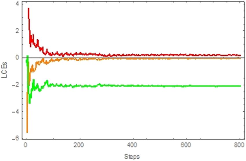
190 Teflah Alresheedi and Ali Allahem
assembly processes, and self-organization [10]. In this paper, we use LEs as a significant dynamical to study
the behavior of three different cases in Hide’s coupled dynamo model. These cases represent the most
common flows that demonstrate how the flow acts when the parameters are changed.
2 Methodology and preliminary results
In this study, we used the LEs as a significant dynamical tool for studying the stability of non-stationary
solutions of ODEs. Moreover, we introduced a novel set of some nonlinear ODEs that have been investigated
by Hide et al. [18], who explained the system by using many differential equations:
x˙ = x( y − 1) − βz ,
y˙ = α(1 − x 2) − κy , (1)
z˙ = x − λz ,
where ẋ , ẏ , and ż are dependent variables on time. ẋ is the electric current of the dynamical system, ẏ is the
disk angular rotation rate, and ż is the motor angular speed. Also, as shown in (1), there are four parameters
denoted as β , α, κ , and λ , which are used to make control for a dynamical system. β is used to measure the
armature inverse moment, α is used to measure the applied couple, and λ and κ are used to measure the
mechanical friction occurring in the motor and disk [19].
Moroz [20] and Hide et al. [18] studied the equilibrium point stability by determining the system steady
dx dy dz
equilibrium. Suppose that , , = 0, then (1) becomes
dt dt dt
x( y − 1) − βz = 0, (2)
α(1 − x 2) − κy = 0, (3)
x − λz = 0. (4)
From (4), we get x = λz . By substituting x = λz into (2), we obtain
λz( y − 1) − βz = 0,
z[λ( y − 1) − β] = 0.
Thus, we get either z = 0 or λ( y − 1) = β . Consequently, we get y = 1 + β / λ .
From these equations, we can see that the first steady state that satisfies all parameters values of λβ , α ,
and κ has the form:
(x , y , z ) = 0, , 0.
α
(5)
κ
In system (1), the current cannot flow as x = 0; the result shows that the motor is stationary z = 0 while
the disk spins. The slow torque is given by the mechanical friction to make a balance between the applied
β
couples [18]. To get the second steady state, we substitute y = 1 + λ into (3). Hence, we get
β
α(1 − x 2) − κ 1 + = 0,
λ
κβ
(α − αx 2) − κ − = 0,
λ
β
(αx 2) = α − κ 1 + = 0,
λ
β
(x 2) = 1 − κ/α 1 + = 0,
λ
β
x = ± 1 − κ/α 1 + .
λ 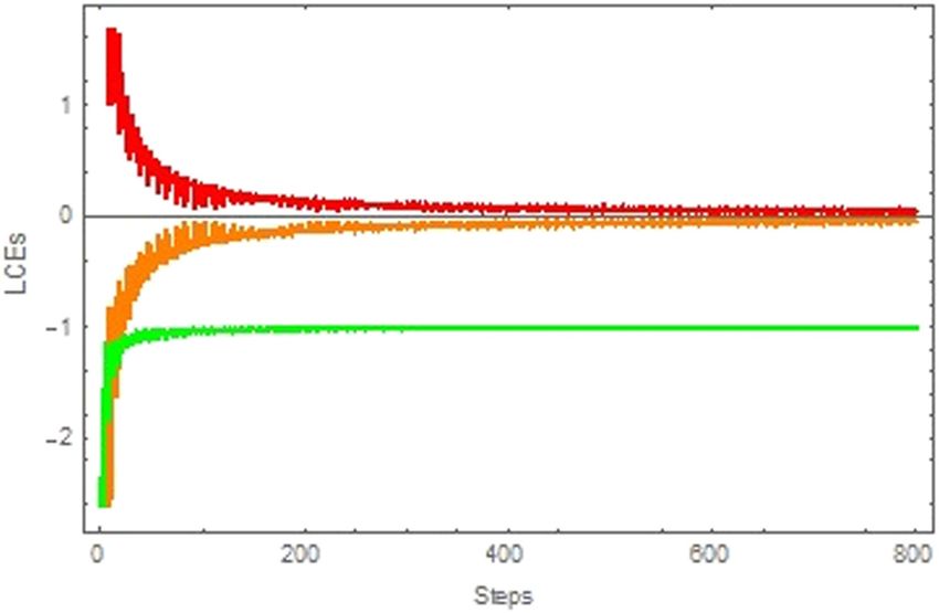
Dynamical study of LEs for Hide’s coupled dynamo model 191
β
Also, we substitute y = 1 + λ
into (2). Hence, we get
β β x = z .
x 1 + − 1 − βz = 0, x = βz ,
λ λ λ
Thus, the second steady-state is in the form:
κ β β x
(x , y , z ) = x = ± 1 − 1 + , 1 + , = E±. (6)
α λ λ λ
2.1 Linear stability of the first steady state
As we have seen that the first steady state is in the form:
(x , y , z ) = 0, , 0.
α
(7)
κ
To study the stability of the first steady state from (5) and (6), the linearization method is applied. Then,
the Jacobi matrix that ends with eigenvalue is as follows:
1 α α − 1 − λ − (4β) .
2
σ1 = −κ , σ2.3 = −1−λ± (8)
2 κ κ
The study of the first steady-state stability analysis of (5) stated two cases. First, the solution becomes stable
when all the three eigenvalues have a real part with negative signs. Second, the change occurs in the
stability when at least one of the real parts of the eigenvalue changes its sign.
2.2 Linear stability of the second steady state
The second steady state can be written as follows:
κ β β x
(x , y , z ) = x = ± 1 − 1 + , 1 + , = E±. (9)
α λ λ λ
The linear stability of (1) applied in the second equilibrium point (5) shows that the Jacobian matrix ends
with cubic eigenvalues equation:
σ3 + aσ 2 + bσ + c = 0,
where a , b, c are equal to
β βk
a=κ+λ− , b = 2(α − κ ) + kλ − 3 , c = 2(αλ − κλ + κβ).
λ λ
The Hopf bifurcation in (5) occurs, when ab = c , and b > 0.
3 Numerical results and discussion
In this study, we introduced the LE as a dynamical tool to demonstrate the behavior of the dynamical
systems. We used the change in the choice of parameters to study the change in the behavior of systems,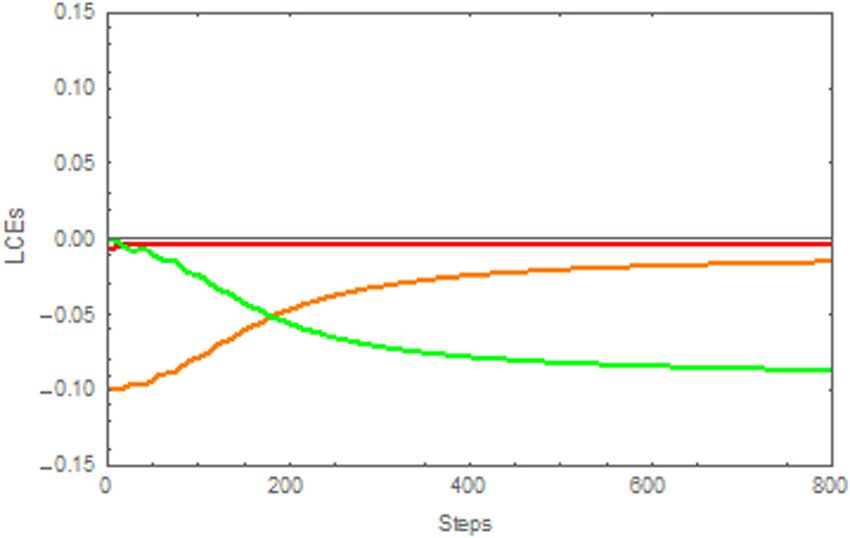
192 Teflah Alresheedi and Ali Allahem
α
β− κ
space. Our numerical results represent the convergence of the LEs for Hide’s model of periodic flow,
regular flow, and chaotic flow. Also, we can see that the LEs give the convergence of trajectories in each
dimension of the attractor depending on changing some selected parameters. In order to integrate the
equation of system (1), we applied the most popular numerical method, i.e., the fourth-order Runge-Kutta
method with an effective time step. Next, the results for a certain choice of parameter values are shown.
3.1 Convergence plot of LEs for Hide’s model of periodic flow
The Hide flow is shown in equation (1). In all calculations that have been shown in this section, we used
Hide’s parameters λ = 0, κ = 0.1, β = 1, and α = 0.10. Our provided numerical results all the time
approaches to the solution given by (1) for all the values of parameters λ , β , α , and κ . We introduced all
output simulated results based on the Mathematica software. In this section, we start with the case λ = 0,
which is physically unrealistic; we analyzed the convergence plot of the LEs for Hide’s model as shown in
Figure 1. There are two isolated periodic orbit examples that are given for the parameter values as repre-
sented in Figure 1, the parameter values are λ = 0, κ = 0.1, β = 1, α = 0.10 and initial conditions are
x(0) = 0, y(0) = 1, z(0) = 0.81. In Figure 1, when parameters κ = 0.1 and α has a value more than 0.1, the
periodic solution occurs. Also, we can see that the convergence of LEs as a periodic flow in the following
coordinates x , y , and z (red, orange, green). Moreover, when α increases, the periodic solution also
increases [18]. In addition, from our results, we can see that the flow wraps around the x -axis, and the
initial conditions have a significant effect on the convergence of the LEs in the dynamical systems [22].
3.2 Convergence of the LEs for Hide’s model of regular flow
In this section, we examined Hide’s parameter values β = 1, α = 50, λ = 0, κ = 0.1, and the initial conditions
are x(0) = 0, y(0) = 4.9, and z(0) = 5.64. The convergence for the above initial condition warps around the
y -axis as shown in Figure 2. As we know that with an increases of α to 50, the periodic flow expands in the
size. Hence, the several solution states are possible, and these solutions depend on the initial conditions.
The LE convergence and the periodic solution number raised as the value of α is increased [22] as shown
in Figure 2. The flow is regular and expands in the size until bends out of y = 2 , as the α increased and
the values of convergence tend to be positive as observed in Figure 2. Moreover, as shown in Figure 2,
the convergence at this initial condition seems to be mostly regular flow.
Figure 1: The convergence plot of the LEs for Hide’s model where initial conditions and parameter values x0 = {0, 1, 0.81}, β = 1 ,
α = 0.10, λ = 0, κ = 0.1 .Dynamical study of LEs for Hide’s coupled dynamo model 193
Figure 2: The convergence plot of the LEs for Hide’s model where initial conditions and parameter values x0 = {0, 4.9, 5.641},
β = 1 , α = 50, λ = 0, κ = 0.1 .
Also, we can show that Figure 2 exhibited more and more periodic solutions while there is an increase
in the value of α .
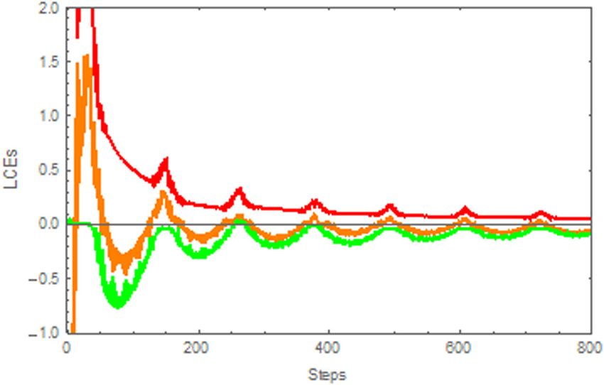
3.3 Convergence of the LEs for Hide’s model of chaos flow
Now, in this section, we introduced two isolated cases of Hide’s parameter values. The first case has parameters
given as β = 2 , α = 20, λ = 1.2 , κ = 1, with initial conditions x(0) = −0.1, y(0) = 5.1, z(0) = −0.34715835.
Also, the second case has parameters given as β = 1.01, α = 100, λ = 1, κ = 1, with initial conditions
x(0) = 0.2 , y(0) = 0.1, z(0) = 0.59. It is clear that the flow in both cases bends around the y -axis as shown
in Figures 3 and 4, which in turn indicate the behavior of chaotic. The chaotic behavior has appeared if λ ≠ 0 for
all of these numerical results. Also, the system of the LEs converges to negative, positive, and zero values, which
is a clear indication of chaotic behavior [23]. In addition, the chaos presence depends on the negative value of
the LEs [24]. Furthermore, the common characteristic of driven systems is the long time needed for the con-
vergence of the LEs [25]. Moreover, from the figures, we can see that when the value of α increased from 20 to
100, the convergence of the LEs becomes more and more regular and periodic [22]. The two cases are considered
as two examples of chaotic behavior as shown in Figures 3 and 4. Furthermore, the chaotic solutions are shown
Figure 3: The convergence plot of the LEs for Hide’s model with initial conditions and parameter values x0 = {−0.1, 5.1,
−0.34715835}, β = 2, α = 20, λ = 1.2, κ = 1 .194 Teflah Alresheedi and Ali Allahem
Figure 4: The convergence plot of the LEs for Hide’s model with initial conditions and parameter values x0 = {0.2, 0.1, 0.59},
β = 1.01 , α = 100, λ = 1 , κ = 1 .
by increasing α to 100 and λ = 1; these solutions go and back between the two unstable periodic cycles which
introduce chaotic attractor similar to the well-known Lorenz attractor [22].
4 Conclusion
A novel set of nonlinear ODEs developed by Hide et al. has been studied by using a significant dynamical
tool that so-called LEs. Due to the significance of these equations and its rich behavior of these equations,
numerous studies that have an interest in this method have been published. One of the key objectives of this
study is to return to Hide et al. and to put their result in perspective as well as to provide an interpretation
and numerical description of these findings. In this study, we introduced the use of the LEs, which is a great
tool to measure the nearby trajectories in the dynamical system. Also, from the theoretical results that have
been found and with the aid of computational methods, we used Hide’s coupled dynamo model and code
up the LEs in three cases of periodic flow, regular flow, and chaos flow. In addition, we have compared
between these systems in logic connections and proved it in this study. An analysis and description of
the dynamics of the system in the figure including the periodic, regular, and chaos flows are obtained.
Moreover, in this study, we showed the convergence of the LEs for the Hide dynamo model depends on the
change in the initial conditions and some parameter values. In addition, we showed that the system
behavior is based on its sensitivity to the four parameters (β , α , κ , λ) and the initial conditions. Three cases
such as the periodic flow, regular flow, and chaotic flow are presented here. Further research in the future
should include the determination of various forms of periodic orbit bifurcation that can be found numeri-
cally. Another idea is to detect the chaotic behavior by adding the alien attractors and the LE. In addition,
further experiments with various parameter values and initial conditions can be investigated.
Acknowledgments: The authors would like to thank the anonymous referees and the handling editor for
their careful reading and for relevant remarks/suggestions which helped them to improve the paper.
The authors gratefully acknowledges Qassim University.
Author contributions: All authors contributed equally.
Conflicts of interest: The authors declare no conflict of interest.
Data availability statement: No data were used to support this study.Dynamical study of LEs for Hide’s coupled dynamo model 195
References
[1] M. Balcerzak, D. Pikunov, and A. Dabrowski, The fastest, simplified method of Lyapunov exponents spectrum estimation for
continuous-time dynamical systems, Nonlinear Dyn. 94 (2018), 3053–3065, DOI: https://doi.org/10.1007/s11071-018-
4544-z.
[2] T. M. Janaki and G. Rangarajan, Lyapunov exponents for continuous-time dynamical systems, J. Indian Inst. Sci. 78 (1998),
267–274.
[3] P. C. Muller, Calculation of Lyapunov exponents for dynamic systems with discontinuities, Chaos Solitons Fractals 5 (1995),
1671–1681, DOI: https://doi.org/10.1016/0960-0779(94)00170-U.
[4] V. Oseledets, Oseledets theorem, Scholarpedia 3 (2008), 1846, DOI: http://dx.doi.org/10.4249/scholarpedia.1846.
[5] G. Benettin, L. Galgani, A. Giorgilli, and J. M. Strelcyn, Lyapunov characteristic exponents for smooth dynamical systems
and for hamiltonian systems; A method for computing all of them. Part 2: Numerical application, Meccanica 15 (1980),
21–30, DOI: https://doi.org/10.1007/BF02128237.
[6] R. Brown, P. Bryant, and H. D. I. Abarbanel, Computing the Lyapunov spectrum of a dynamical system from an observed
time series, Phys. Rev. A 43 (1991), 2787–2806, DOI: https://doi.org/10.1103/PhysRevA.43.2787.
[7] I. Goldhirsch, P. L. Sulem, and S. A. Orszag, Stability and Lyapunov stability of dynamical systems: A differential approach
and a numerical method, Phys. D Nonlinear Phenom. 27 (1987), no. 3, 311–337, DOI: https://doi.org/10.1016/0167-
2789(87)90034-0.
[8] L. Dieci, R. D. Russell, and E. S. Van Vleck, On the computation of Lyapunov exponents for continuous dynamical systems,
SIAM J. Numer. Anal. 34 (1997), 402–403, DOI: https://doi.org/10.1137/S0036142993247311.
[9] P. Melby, N. Weber, and A. Hilbler, Dynamics of self-adjusting systems with noise, Chaos 15 (2005), 033902,
DOI: https://doi.org/10.1063/1.1953147.
[10] V. Gintautas, G. Foster, and A. W. Hilbler, Resonant forcing of chaotic dynamics, J. Stat. Phys. 130 (2008), 617–629,
DOI: https://doi.org/10.1007/s10955-007-9444-4.
[11] A. Choucha, S. M. Boulaaras, D. Ouchenane, and A. Allahem, Global existence for two singular one-dimensional nonlinear
viscoelastic equations with respect to distributed delay term, J. Funct. Spaces 2021 (2021), 6683465, DOI: https://doi.org/
10.1155/2021/6683465.
[12] A. Allahem, Analytical solution to normal forms of Hamiltonian systems, Math. Comput. Appl. 22 (2017), no. 3, 37,
DOI: https://doi.org/10.3390/mca22030037.
[13] S. Otmani, S. Boulaaras, and A. Allahem, The maximum norm analysis of a nonmatching grids method for a class of
parabolic p(x)-Laplacian equation, Boletim Sociedade Paranaense de Matematica (2019), (in press).
[14] A. Allahem, New derived systems of Hide’s coupled dynamo model, Eur. J. Pure Appl. Math. 10 (2017), no. 4, 858–870.
[15] A. Allahem, Synchronized chaos of a three-dimensional system with quadratic terms, Math. Probl. Eng. 2020 (2020),
8813736, DOI: https://doi.org/10.1155/2020/8813736.
[16] S. Boulaaras and A. Allahem, Two-dimensional mathematical model of the transport equations of some pollutants and
their diffusion in a particular fluid, J. Intell. Fuzzy Syst. 38 (2020), no. 3, 2457–2467.
[17] Dynamical systems – Latest research and reviews, Nature, https://www.nature.com/subjects/dynamical-systems
[Accessed July 7, 2020].
[18] R. Hide, A. C. Skeldon, and D. J. Acheson, A study of two novel self-exciting single-disk homopolar dynamos: theory,
Proc. R. Soc. A Math. Phys. Eng. Sci. 452 (1996), no. 1949, 1369–1395, DOI: https://doi.org/10.1098/rspa.1996.0070.
[19] R. Hide, The nonlinear differential equations governing a hierarchy of self-exciting coupled Faraday-disk homopolar
dynamos, Phys. Earth Planet. Inter. 103 (1997), no. 3–4, 281–291, DOI: https://doi.org/10.1016/S0031-9201(97)00038-1.
[20] I. M. Moroz, Synchronised behavior in three coupled Faraday disk homopolar dynamos, in: J. L Lumley (ed.), Fluid
Mechanics and the Environment: Dynamical Approaches, Lecture Notes in Physics, vol. 566, Springer, Berlin, Heidelberg,
pp. 225–238, DOI: https://doi.org/10.1007/3-540-44512-9_12.
[21] E. Almohaimeed and A. Allahem, Poincare section for Hide coupled dynamo model, J. Inf. Sci. Eng. 36 (2020), no. 6,
1211–1221.
[22] N. Mezouar, S. M. Boulaaras, and A. Allahem, Global existence of solutions for the viscoelastic Kirchhoff equation with
logarithmic source terms, Complexity 2020 (2020), 105387, DOI: https://doi.org/10.1155/2020/7105387.
[23] M. P. John and V. M. Nandakumaran, Studies on the effect of randomness on the synchronization of coupled systems and
on the dynamics of intermittently driven systems, PhD Dissertation, Cochin University of Science and Technology, 2009.
[24] B. Muthuswamy and P. Kokate, Memristor-based chaotic circuits, IETE Tech. Rev. (Institution Electron. Telecommun. Eng.
India) 26 (2009), no. 6, 417–429.
[25] B. Muthuswamy, Implementing memristor based chaotic circuits, Int. J. Bifurc. Chaos 20 (2010), no. 5, 1335–1350,
DOI: https://doi.org/10.1142/S0218127410026514.You can also read