Diffusing wave spectroscopy: A unified treatment on temporal sampling and speckle ensemble methods
←
→
Page content transcription
If your browser does not render page correctly, please read the page content below
Diffusing wave spectroscopy: A unified
treatment on temporal sampling and
speckle ensemble methods
Cite as: APL Photonics 6, 016105 (2021); https://doi.org/10.1063/5.0034576
Submitted: 22 October 2020 . Accepted: 23 December 2020 . Published Online: 19 January 2021

  Jian Xu,    Ali K Jahromi, and Changhuei Yang

ARTICLES YOU MAY BE INTERESTED IN

Interferometric speckle visibility spectroscopy (ISVS) for human cerebral blood flow
monitoring
APL Photonics 5, 126102 (2020); https://doi.org/10.1063/5.0021988

Beating temporal phase sensitivity limit in off-axis interferometry based quantitative phase
microscopy
APL Photonics 6, 011302 (2021); https://doi.org/10.1063/5.0034515

Integrated nanophotonics for the development of fully functional quantum circuits based
on on-demand single-photon emitters
APL Photonics 6, 010901 (2021); https://doi.org/10.1063/5.0031628

APL Photonics 6, 016105 (2021); https://doi.org/10.1063/5.0034576                         6, 016105

© 2021 Author(s).
APL Photonics                                                                                   ARTICLE            scitation.org/journal/app

    Diffusing wave spectroscopy: A unified treatment
    on temporal sampling and speckle ensemble
    methods
    Cite as: APL Photon. 6, 016105 (2021); doi: 10.1063/5.0034576
    Submitted: 22 October 2020 • Accepted: 23 December 2020 •
    Published Online: 19 January 2021

    Jian Xu,a)         Ali K Jahromi,            and Changhuei Yang

    AFFILIATIONS
    Department of Electrical Engineering, California Institute of Technology, Pasadena, California 91125, USA

    a)
         Author to whom correspondence should be addressed: jxxu@caltech.edu

    ABSTRACT
    Diffusing wave spectroscopy (DWS) is a well-known set of methods to measure the temporal dynamics of dynamic samples. In DWS,
    dynamic samples scatter the incident coherent light, and the information of the temporal dynamics is encoded in the scattered light. To
    record and analyze the light signal, there exist two types of methods—temporal sampling methods and speckle ensemble methods. Tem-
    poral sampling methods, including diffuse correlation spectroscopy, use one or multiple large bandwidth detectors to sample well and
    analyze the temporal light signal to infer the sample temporal dynamics. Speckle ensemble methods, including speckle visibility spec-
    troscopy, use a high-pixel-count camera sensor to capture a speckle pattern and use the speckle contrast to infer sample temporal dynamics.
    In this paper, we theoretically and experimentally demonstrate that the decorrelation time (τ) measurement accuracy or signal-to-noise
    ratio (SNR) of the two types of methods has a unified and similar fundamental expression based on the number of independent observ-
    ables (NIO) and the photon flux. Given a time measurement duration, the NIO in temporal sampling methods is constrained by the
    measurement duration, while speckle ensemble methods can outperform by using simultaneous sampling channels to scale up the NIO
    significantly. In the case of optical brain monitoring, the interplay of these factors favors speckle ensemble methods. We illustrate that
    this important engineering consideration is consistent with the previous research on blood pulsatile flow measurements, where a speckle
    ensemble method operating at 100-fold lower photon flux than a conventional temporal sampling system can achieve a comparable
    SNR.
    © 2021 Author(s). All article content, except where otherwise noted, is licensed under a Creative Commons Attribution (CC BY) license
    (http://creativecommons.org/licenses/by/4.0/). https://doi.org/10.1063/5.0034576

    I. INTRODUCTION                                                           and analyze the recorded light signal to infer the information of
                                                                              CBF.
          Diffusing wave spectroscopy (DWS)1,2 is a well-established                Since the dynamic of the light signal is tied to the temporal
    approach that is used to measure the temporal dynamical proper-           dynamic of the dynamic sample, there exist two sets of methods to
    ties of dynamic samples, such as in vivo blood flow monitoring,3          measure the light signal to attain the information of the temporal
    air turbulence quantification,4 and particle diffusion in liquid solu-    dynamic—one is to use temporal sampling methods and the other
    tion.5 A common experimental setting of DWS is to use a coher-            one is to use speckle ensemble methods. Both methods share similar
    ent laser source to illuminate the dynamic sample and measure the         light illumination systems [Fig. 1(a)], and the difference is that they
    scattered light. The scattered light forms a dynamic speckle pattern      collect and analyze the light signal differently.
    in which the information of the sample dynamics is encoded, and                 Temporal sampling methods, including diffuse correlation
    therefore, the sample temporal dynamics can be inferred by analyz-        spectroscopy (DCS),1,3–5,7 utilize one or multiple large bandwidth
    ing the intensity of scattered light. Recently, DWS has been applied      detectors to record the intensity fluctuation of one or a few speckle
    in biomedical and clinical areas, especially in monitoring cerebral       grains and analyze the temporal signal to reconstruct the infor-
    blood flow (CBF).3,6–11 In such applications, researchers typically       mation of the temporal dynamics. The recorded intensity fluc-
    utilize red or near-infrared light to illuminate the brain through        tuation trace I(t), where t denotes time, is autocorrelated and
    skin, probe the dynamic scattering light that interacts with the brain,   normalized to approximate the intensity correlation function

APL Photon. 6, 016105 (2021); doi: 10.1063/5.0034576                                                                                        6, 016105-1
© Author(s) 2021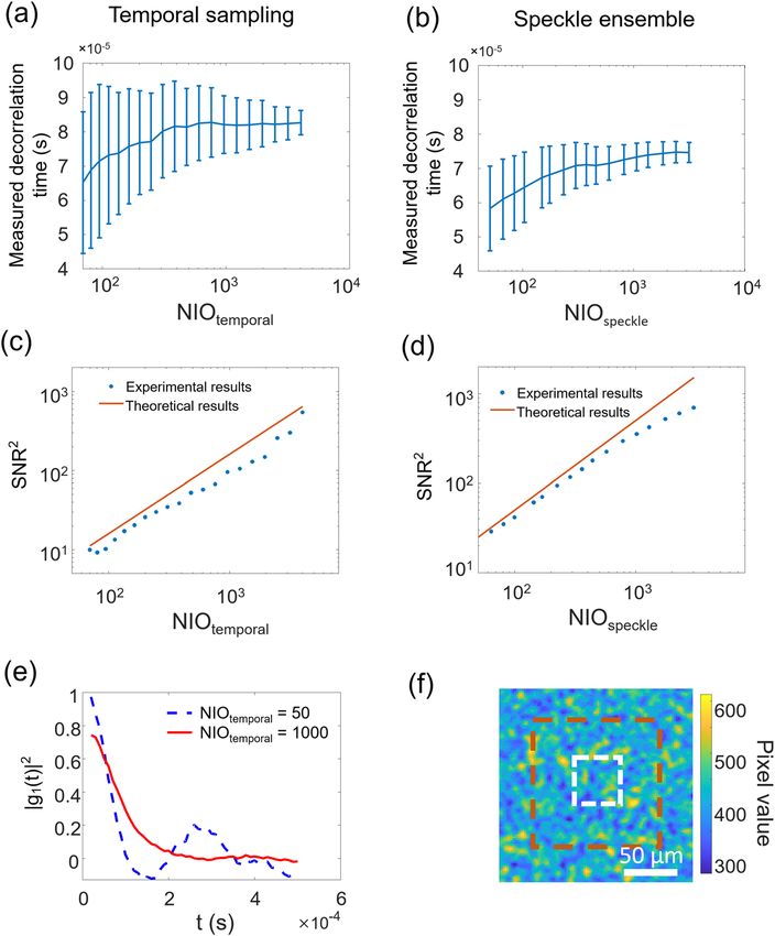
APL Photonics                                                                                                    ARTICLE            scitation.org/journal/app

                                                                                                     Typical speckle ensemble methods, including speckle visibil-
                                                                                              ity spectroscopy (SVS,14,15 also known as speckle contrast spec-
                                                                                              troscopy9 ) and laser speckle contrast imaging (LSCI),11,16 use a cam-
                                                                                              era sensor as a detector to record a frame of the speckle pattern. The
                                                                                              camera exposure time is longer than the speckle decorrelation time
                                                                                              (in experiments, this is generally set at least one order of magnitude
                                                                                              longer than the decorrelation time), and therefore, multiple different
                                                                                              speckle patterns sum up within the exposure time, yielding a blurred
                                                                                              speckle pattern. The decorrelation time is then calculated from the
                                                                                              degree of blurring—more specifically, from the speckle contrast over
                                                                                              the speckles in the whole frame. The speckle contrast γ relates with
                                                                                                                              T
                                                                                              g 1 (t) in the form of γ2 = ∫0 2(1 − Tt )∣g1 (t)∣2 dt (see Ref. 14 and
                                                                                              the Appendix). From the measured speckle pattern, we can calcu-
                                                                                              late γ to obtain g 1 (t) and, consequently, obtain information on the
                                                                                              sample dynamics [Fig. 1(b)]. Generally, a shorter decorrelation time
                                                                                              will cause a lower contrast speckle frame. Figure 1(d) gives exam-
                                                                                              ples of speckle frames with a short decorrelation time and a long
                                                                                              decorrelation time.
                                                                                                     Since the aforementioned two sets of methods share simi-
                                                                                              lar optical illumination but use different detection principles, it is
                                                                                              worthwhile to jointly analyze the fundamental limitations and the
      FIG. 1. An overview of the scattered light dynamics measurement. (a) After the          performance of the two methods. Some previous research studies
      illumination light interacts with the dynamic scatterers, the scattered light forms a   have investigated the performance of the two individual methods
      set of dynamic speckle patterns. Temporal sampling methods usually use a high           for several aspects. For instance, Ref. 17 discusses the effect of finite
      speed detector to record the intensity temporal fluctuation, while speckle ensemble     sampling time in temporal sampling methods, Refs. 18 and 19 build
      methods usually use a camera sensor to record the speckle patterns. (b) Temporal        up comprehensive noise models for temporal sampling methods,
      sampling methods calculate the autocorrelation function of the recorded intensity
                                                                                              and Ref. 15 discusses the effect of shot noise on speckle ensemble
      fluctuation to obtain the speckle decorrelation time. Speckle ensemble methods
      calculate the speckle contrast and use mathematical models to obtain the speckle        methods. Here, we jointly realize a unified analysis on the perfor-
      decorrelation time. In both methods, the calculated speckle decorrelation time is       mance of the two sets of methods and show the equivalence of
      used to infer the scattering dynamics. (c) Examples of field decorrelation func-        the measurement accuracy of the two methods. Interestingly, we
      tions with short and long decorrelation times in temporal sampling methods. (d)         were able to find a unified expression for the two methods with
      Examples of speckle frames with a short and a long decorrelation times in speckle       respect to the measurement accuracy. The accuracy of decorrela-
      ensemble methods.
                                                                                              tion time measurements from both sets of methods is determined
                                                                                              by the number of independent observables (NIO) and the amount
                                                                                              of photon flux. In temporal sampling methods, the NIO is the num-
                                                                                              ber of decorrelation events recorded by the detector, while in speckle
    g 2 (t), i.e., g2 (t) = ⟨I(t⟨I(t
                                 1 )I(t1 −t)⟩
                                              where ⟨⋅⟩ denotes the average over              ensemble methods, it is the number of collected speckle grains. The
                                       2
                                     1) ⟩
                                                                                              NIO equivalence of the two methods is fundamentally attributable
    time variable t 1 . According to the Siegert relation,12 the inten-
                                                                                              to the equivalence of the spatial speckle ensemble and temporal
    sity correlation function g 2 (t) is g 2 (t) = 1 + ∣g 1 (t)∣2 , where g1 (t)
                                                                                              ensemble.
    = ⟨E(t⟨E(t
           1 )E(t1 −t)⟩
                 2
               1) ⟩
                        is the electric field [E(t)] correlation function. The                       Under typical experimental conditions where photon shot
    speckle decorrelation time is introduced to describe the time scale                       noise is the dominant noise source in the measurement, the two
    during which decorrelation happens. Generally, speckle decorrela-                         sets of methods should provide decorrelation measurements with
    tion time τ is defined as the time point when the temporal autocor-                       similar accuracy, given the same NIO and photon flux. In the exper-
    relation function g 1 (t) drops below a certain threshold. A common                       iment, we observed that speckle ensemble methods generally have a
    model is g 1 (t) = exp(−∣t∣/τ),13 where the scatterers are assumed to                     higher signal-to-noise ratio (SNR) in CBF measurements when the
    undergo homogeneous random motion (Brownian motion), and the                              sampling rate is fixed. A speckle ensemble method operating at a
    time instant that g 1 (t) drops to 1/e is defined as the decorrelation                    100-fold lower photon flux than a conventional temporal sampling
    time (also known as temporal coherence time). There are also other                        method can still achieve a comparable SNR, which is consistent with
    models such as the one where g 1 (t) follows the Gaussian function as                     the results in our previous work.20 This is because camera sensors
    g 1 (t) = exp(−t 2 /τ 2 )13 where the scatterers are assumed to undergo                   used in speckle ensemble methods typically have very large pixel
    inhomogeneous random motion, but in general, they should not                              counts and thereby allow us to achieve a large NIO within the lim-
    affect the decorrelation quantification much. The autocorrelation                         ited measurement time. In contrast, temporal sampling methods,
    function of the intensity fluctuation signal can be used to approxi-                      which typically use a single-photon-counting module (SPCM) or
    mate g 2 (t), and it can then be calculated to obtain the speckle decor-                  other high speed single detectors, tend to lead to a relatively small
    relation time and scattering dynamics [Fig. 1(b)]. Figure 1(c) gives                      NIO within the limited measurement time. There have been previ-
    examples of field decorrelation functions with a short decorrelation                      ous21 and recent22 efforts in using multiple detectors to boost the
    time and a long decorrelation time.                                                       effective NIO for temporal sampling methods. However, to date,

APL Photon. 6, 016105 (2021); doi: 10.1063/5.0034576                                                                                                          6, 016105-2
© Author(s) 2021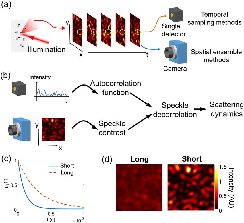
APL Photonics                                                                                            ARTICLE            scitation.org/journal/app

    the number of parallel high-speed detectors deployed in such                      ΔT needs to be on the order of microseconds or smaller (one order
    a fashion is still orders of magnitude lower than the number                      of magnitude smaller than the decorrelation time). In turn, this
    of pixels available in the standard commercial cameras used in                    implies that temporal sampling methods require substantially fast
    speckle ensemble methods. As we shall explain in Sec. II, tem-                    detectors.
    poral sampling methods require much more and much faster                                Spatially, the two types of DWS methods have a similar opti-
    raw data measurements to generate the same NIO as speckle                         mization criterion. In both cases, one should match the detector
    ensemble methods.                                                                 active pixel area to the typical speckle grain size at the detector
                                                                                      plane. In speckle ensemble methods, this may not always be prac-
    II. THEORY                                                                        tical. In the event that the speckle grain size is larger than the cam-
                                                                                      era pixel size, we can use the mutual coherence function23 to esti-
          For the following analysis, we will use optical brain monitoring
                                                                                      mate the speckle grain size. A common parameter of interest for
    as the specific reference example. We choose to do this so that we can
                                                                                      both systems is N τ , a dimensionless number, which is the aver-
    map some of the parameters involved in interpretable experimen-
                                                                                      age number of collected signal photons in one speckle grain per
    tal parameters and promote a better understanding of the factors at
                                                                                      time τ.
    play. The analysis itself is general and can be applied to most, if not
                                                                                            For temporal sampling methods that use a single detector, the
    all, DWS applications.
                                                                                      SNR of the measured decorrelation time τ, which is defined as the
          To start the quantitative analysis on the two sets of DWS meth-
                                                                                      expected decorrelation time τ divided by error(τ) (error of τ in the
    ods, let us first define the various time scales involved in the mea-
                                                                                      measurement), has the form of [see Eq. (A36) in the Appendix]
    surement process (Fig. 2). T̃ denotes the total duration for the mea-
    surement process. For a brain monitoring experiment, T̃ represents                                       √
                                                                                                                 2          1           √
    the entire duration of the experiment when measurements are made.                          SNRtemporal =       √                       NIOtemporal .   (1)
                                                                                                               e          2     2 τ
    While it is not used in our subsequent analysis of SNR, we formally                                              1+       + 2
    define it here so that we are cognizant of this overarching time scale                                               Nτ Nτ ΔT
    in the entire measurement process. τ equals the speckle field decor-
    relation time and it is the quantity that both sets of methods seek to            Here, NIOtemporal is defined as 2T/τ, where the constant 2 in 2T/τ
    measure. τ can change over the entire duration of T̃, and we segment              is introduced to match the conversion between g 1 (t) and g 2 (t).
    T̃ into increments of T in order to generate a time trace of τ measure-           Intuitively, NIOtemporal is the ratio between the measurement dura-
    ments (see the top plot of Fig. 2 for illustration). T should be chosen           tion T and the decorrelation time τ, which denotes the number
    so that it is substantially larger than τ and substantially smaller than          of decorrelation events. The detailed derivation is shown in the
    the time scale at which τ is changing. For temporal sampling meth-                Appendix.
    ods, there is an additional factor ΔT involved—1/ΔT is the rate at                     In speckle ensemble methods, the NIO is equal to the number of
    which raw intensity measurements are acquired. ΔT is substantially                independent speckle grains captured by the camera sensor. The SNR
    smaller than τ, as temporal sampling methods require multiple mea-                of the measured decorrelation time τ has the form of [see Eq. (A25)
    surements to determine τ. 1/T is referred to as the sampling rate, or             of the Appendix]
    more specifically, it is the rate at which an estimate of τ is generated.                                  1    1 √
    The terminology can be confusing and 1/T should not be confused                              SNRspeckle = √           NIOspeckle
                                                                                                                2 1+ 1
    with 1/ΔT, which is the raw data sampling rate in temporal sampling                                              Nτ
    methods. ΔT is particularly important during system design, as tem-                                        1        1       √
    poral sampling methods require ΔT to be substantially smaller than                                      =√ √                    NIOspeckle .           (2)
                                                                                                                2       2    1
    τ so that the intensity fluctuation can be adequately sampled. As τ in                                          1+     + 2
    brain monitoring is typically on the order of tens of microseconds,                                                 Nτ Nτ

                                                                                      NIOspeckle is the NIO in speckle ensemble methods. The detailed
                                                                                      derivation is shown in the Appendix.
                                                                                            To better interpret this expression, we will briefly describe the
                                                                                      measurement system for which this expression would directly apply
                                                                                      to. Such a measurement system will have a camera with NIOspeckle
                                                                                      pixel counts. Each pixel will collect light from a single speckle grain.
                                                                                      Each pixel will integrate the collected photons over a time duration
                                                                                      of time T and output the result. It is interesting to note that T, the
                                                                                      camera exposure time in speckle ensemble methods, is not explic-
                                                                                      itly expressed in Eq. (2). This is because as long as T is substantially
                                                                                      longer than τ, a single camera frame capture of the independent
                                                                                      speckle grains does not provide any more or less information if T is
                                                                                      further lengthened. In brain monitoring experiments, a typical T can
                                                                                      be set at ∼ 10τ or longer to ensure the following conditions: (i) the
                                                                                      approximation in Eq. (A8) holds, (ii) shot noise dominant detection
                                                                                      condition holds, and (iii) camera pixels are not saturated. Hence, T
            FIG. 2. An illustration of various time scales defined in the analysis.
                                                                                      in speckle ensemble methods is typically more than 100 times larger

APL Photon. 6, 016105 (2021); doi: 10.1063/5.0034576                                                                                                 6, 016105-3
© Author(s) 2021
APL Photonics ARTICLE scitation.org/journal/app
than ΔT in temporal sampling methods since typically ΔT is less We can see that temporal sampling methods require substantially
than 0.1τ. In turn, this implies that speckle ensemble methods can more measurements to achieve the similar SNR as speckle ensemble
employ relatively slow commercially available cameras. methods since 2ΔT τ
is substantially less than unity.
Equations (1) and (2) reveal that the two sets of methods have Yet, another way through which we can interpret the two equa-
similar dependencies on signal photon counts per speckle per decor- tions [Eqs. (1) and (2)] is to recast them in terms of the total number
relation time N τ and NIO. From a mathematically perspective, we of photons collected (N photons ). For speckle ensemble methods, since
estimate a statistical parameter (decorrelation time τ) from the data, Nphotons = NIOspeckle × Nτ × Tτ , the SNR expression is given by
and the accuracy (SNR of τ) of the estimation increases with the
number of independent sampling points (NIO in this case) accord- √
1 1 Nphotons τ
ing to the central limit theorem. In the regime where the photon flux SNRspeckle = √ √ . (5)
is high enough that N τ ≫ 1, the center term in both Eqs. (1) and (2) 2 2 1 Nτ T
1+ +
reduces to unity, and both SNR expressions are directly proportional Nτ Nτ2
to the square root of NIO. In this regime, the shot noise is negli-
gible compared to the light fluctuations induced by the scatterers’ For temporal sampling methods, since N photons = NIOtemporal
dynamics. On the other hand, in the regime where N τ is compara- × N τ , the SNR expression is given by
ble to or smaller than unity, the center term in both expressions can √
√
negatively impact the SNR—the impact of photon shot noise is now 2 1 Nphotons
more strongly felt. As ΔT is much smaller than τ, SNRtemporal gener- SNRtemporal = √ . (6)
e 2 2 τ Nτ
ally is far worse than SNRspeckle in this regime. In the grand scheme 1+ + 2
Nτ Nτ ΔT
of things, this factor is relatively minor. Practically, we simply have
to make sure that the measurements do not operate in this regime.
In the regime where N τ is ≫ 1, we can see that speckle ensemble
Since the SNR “saturates” with respect to N τ when N τ ≫ 1, the
methods require substantially more photons to achieve the same
practical way to perform high accuracy decorrelation time measure-
SNR as temporal sampling methods. In the context of optical brain
ments is to increase the NIO under the photon sufficient condition
monitoring, this situation can occur if (1) the light intensity level is
(N τ ≫ 1).
very high so that the condition for N τ ≫ 1 is met and (2) both spa-
These pairs of equations reveal a number of interesting proper-
tial and temporal methods are constrained to only collect the same
ties for both types of methods.
number of photons. The second condition is highly artificial and
In optical brain monitoring, T is constrained as one cannot
can be dismissed, as a well-designed speckle ensemble system would
increase T beyond the time scale of the physiological changes that
try to collect light from an area as broad as possible and, thus, can
one is trying to measure. As such, NIOtemporal = 2T/τ has an upper
easily exceed the amount of photons that is collected by a temporal
bound. NIOspeckle has no such limitation, as NIO is directly depen-
sampling system.
dent on the number of camera pixels that one can use. Ultimately,
These two types of equational recasting are helpful because they
NIOspeckle is constrained by the total area from which we can collect
highlight the impact of the various factors on the SNR expressions
photons, but this limit is seldom reached in optical brain monitoring
for spatial and temporal ensemble methods.
experiments. For this reason, the SNR for speckle ensemble methods
In the Appendix, we will further examine the SNR expressions
can substantially improve over single detector temporal sampling
for measurement systems that deviate from these designs above. The
methods by simply increasing camera pixel counts.
expression for temporal sampling methods that use multiple parallel
We can also recast the two equations in terms of the amount
detectors is particularly relevant as there have been previous21 and
of measurements made. The total amount of measurements made in
recent22 efforts focused on such a strategy to improve DWS perfor-
T for speckle ensemble methods is M speckle if there are M speckle pixels
mance. In brief, such methods can indeed improve the SNR. How-
used to take the speckle frame and each pixel records one speckle
ever, they still require raw data measurements at high speed (∼ tens
grain. From Eq. (2), this leads to an SNR expression
to hundreds of kHz or more). Moreover, such methods still require
orders of magnitude more measurements to provide a similar SNR
1 1 √ that speckle ensemble methods provide.
SNRspeckle = √ √ Mspeckle . (3)
2 2 1
1+ + 2 III. EXPERIMENT
Nτ Nτ
We performed experiments to verify the SNR equations
[Eqs. (1) and (2)] of decorrelation time measurements in both tem-
The total amount of measurements made in time T for tem-
poral sampling and speckle ensemble methods. The experimental
poral sampling methods is equal to Mtemporal = ΔT T
= 2T
τ
× 2ΔT
τ
setup is shown in Fig. 3. A laser beam (laser model number: Crys-
= NIOtemporal × 2ΔT
τ
. Substituting it in Eq. (1), this leads to an SNR
taLaser, CL671-150, wavelength 671 nm) is coupled to a multimode
expression
fiber FB1, and the output beam from the fiber illuminates the sam-
ple (in the gray dashed line box). The scattered light is collected
√ √
2 1 2ΔT by a 4-f system (L1 and L2) and is split onto a camera (Phantom
SNRtemporal = √ Mtemporal . (4) S640) and an SPCM (PerkinElmer, SPCM-AQRH-14), respectively.
e 2 2 τ τ
1+ + 2 In the diffuser experiment where we verified the models for the
Nτ Nτ ΔT two sets of methods, the light passes a rotating diffuser and a static
APL Photon. 6, 016105 (2021); doi: 10.1063/5.0034576 6, 016105-4
© Author(s) 2021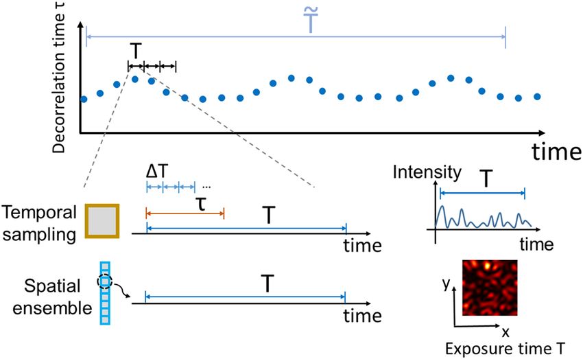
APL Photonics ARTICLE scitation.org/journal/app
diffused light at a source–detector (S–D) separation of 1.5 cm is col-
lected by a large core multimode fiber FB2 (Thorlabs M107L02,
core diameter 1.5 mm, containing 6 × 10⁶ modes) and directed
to the 4-f system. For the biological experiment, a near infrared
(NIR) laser with a long coherence length and stable spectrum will
be preferred over the current laser or a low cost He–Ne laser, as
a typical biological tissue has lower absorption coefficients at NIR
wavelengths.
In the human experiment, the 56 mW laser beam with a
6-mm spot size results in a < 2 mW/mm2 irradiance for skin
exposure—within the limit stipulated by American National Stan-
dard Institute (ANSI). The output of this fiber was channeled to
FIG. 3. Experimental setup. AP—aperture, BS—beam splitter, CAM—camera, the camera. A human protocol comprising all detailed experimental
FB—fiber, FC—fiber coupler, L—lens, ND—neutral density filter, P—polarizer, procedures was reviewed and approved by the Caltech Institutional
R—rotating diffuser, and SPCM—single photon counting module. Review Board (IRB) under IRB protocol 19-0941, informed consent
was obtained in all cases, and safety precautions were implemented
to avoid accidental eye exposure.
diffuser, and the scattered light is directly collected by the 4-f sys- The experimental results confirm our theoretical analysis. We
tem. In the human experiment where we demonstrated the NIO first verified the relation between SNR and NIO, given a fixed pho-
advantage of speckle ensemble methods over temporal sampling ton flux N τ . Figure 4 shows the relation between the SNR and the
methods, the light illuminates the skin of the human subject, and NIO under the photon sufficient case for both temporal sampling
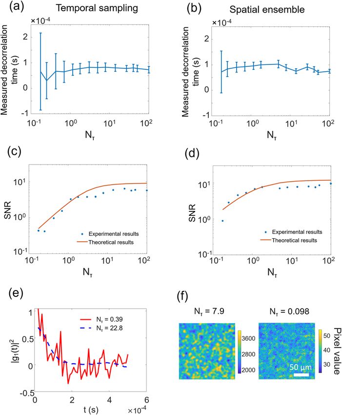
FIG. 4. The performance of temporal
sampling and speckle ensemble meth-
ods with respect to different NIOs.
(a) Temporal sampling measured the
speckle decorrelation time with respect
to varying NIO. The error bar is calcu-
lated from 30 data points. (b) Speckle
ensemble measured the speckle decor-
relation time with respect to varying NIO.
The error bar is calculated from 30 data
points. (c) The square of SNR with
respect to varying NIO in the tempo-
ral sampling methods. (d) The square of
SNR with respect to varying NIO in the
speckle ensemble methods. (e) Exam-
ples of the autocorrelation functions from
intensity temporal fluctuation traces with
different NIOs. (f) An example of a
speckle frame used to calculate speckle
contrast. The box outlined by the red
dashed line indicates a large NIOspeckle ,
and the box outlined by the white dashed
line indicates a small NIOspeckle .
APL Photon. 6, 016105 (2021); doi: 10.1063/5.0034576 6, 016105-5
© Author(s) 2021APL Photonics ARTICLE scitation.org/journal/app
and speckle ensemble methods. In the experiment, N τ is set to be speckle contrast value is 0.124, while the big and small enclosed
∼ 10. The experimentally measured decorrelation times at different boxes provide contrast values of 0.123 and 0.132, respectively. The
NIOs are demonstrated in Figs. 4(a) and 4(b). Both methods can speckle contrast calculated from a small enclosed box gives a rela-
consistently measure the decorrelation time, with less errors as NIO tively large error from the expected contrast. Similar to the temporal
increases. In both methods, the square of the SNR scales up linearly sampling method, here in the speckle ensemble method, a small
with the NIO, as predicted by the theoretical analysis. Due to the enclosed box does not contain the statistically sufficient number of
approximation in the theoretical analysis (see the Appendix) and speckle grains to be representative for all the speckle grains in the
experimental imperfections such as detector noise and non-perfect frame.
control of the diffuser rotating speed, the experimental SNR2 scales We then verified the relation between the SNR and photon
up slower compared to the theoretical line. This results in a gap flux N τ , given a fixed NIO. Figure 5 shows the relation between the
between the experimental dots and the theoretical line in the log–log SNR and N τ when the NIO is set to be 300 for both temporal sam-
plot [Figs. 4(c) and 4(d)]. Figure 4(e) shows examples of the auto- pling and speckle ensemble methods. The experimentally measured
correlation functions from intensity temporal fluctuation traces with decorrelation times at different N τ are demonstrated in Figs. 5(a)
different NIOs. Under such a photon sufficient condition, less NIO and 5(b). In both methods, the SNR does not change much under
will cause the “shape deviation” from the expected autocorrelation the photon sufficient case (N τ > 10), while it starts to decrease when
function. Intuitively speaking, the number of sampled decorrelation N τ is comparable to 1, as shown in Figs. 5(c) and 5(d). Figure 5(e)
events is not statistically sufficient to be representative for the whole shows examples of the autocorrelation functions from intensity tem-
decorrelation process. Figure 4(f) shows a speckle frame from the poral fluctuation traces with different N τ . In this case, a small N τ
speckle ensemble method, with the enclosed red and white boxes will cause more fluctuation in the calculated autocorrelation func-
containing different numbers of speckle grains. The whole frame tion. Different from the case of small NIO where the autocorrelation
FIG. 5. The performance of temporal
sampling and speckle ensemble meth-
ods with respect to different Nτ . (a) Tem-
poral sampling measured speckle decor-
relation time with respect to varying Nτ .
The error bar is calculated from 30 data
points. (b) Speckle ensemble measured
speckle decorrelation time with respect
to varying Nτ . (c) SNR with respect
to varying Nτ in the temporal sampling
methods. The error bar is calculated from
30 data points. (d) SNR with respect
to varying Nτ in the speckle ensemble
methods. (e) Examples of the autocor-
relation functions from intensity tempo-
ral fluctuation traces with different Nτ .
(f) Examples of the speckle frames with
different Nτ .
APL Photon. 6, 016105 (2021); doi: 10.1063/5.0034576 6, 016105-6
© Author(s) 2021APL Photonics ARTICLE scitation.org/journal/app
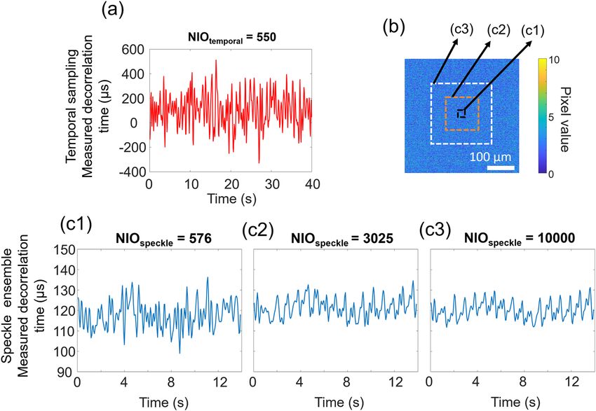
FIG. 6. Human CBF induced speckle
decorrelation time measurement results
from temporal sampling and speckle
ensemble methods. (a) Results from
the temporal sampling method. (b)
A speckle frame from the speckle
ensemble method. The white, orange,
and black boxes enclose 10 000, 3025,
and 576 speckle grains, respectively.
(c1)–(c3) Results from the speckle
ensemble method with different
NIOspeckle .
function remains smooth but has a “shape deviation” from the The reason to the above performance difference between the
expected autocorrelation function, a small N τ here contributes two sets of methods is tied to the achievable NIO. Under the exper-
more “noise” on the calculated autocorrelation function. From imental condition, the photon flux is limited by safety limit. There-
Eqs. (A29) and (A30) in the Appendix, the fluctuation of the fore, a high SNR measurement can only be achieved by a large NIO.
autocorrelation function fundamentally comes from the autocor- In temporal sampling methods, a larger NIO is achieved by mea-
relation operation of the noise in the intensity measurement. suring more decorrelation events (2T/τ), while in speckle ensemble
Figure 5(f) shows speckle frames from the speckle ensemble methods, a larger NIO is achieved by measuring more speckles. Since
method with different N τ . The low N τ speckle frame looks nois- the sampling rate is fixed to 18 Hz (56 ms sampling time) and the
ier than the high N τ frame due to the relatively greater impact speckle decorrelation time is mostly determined by CBF (a decor-
of shot noise when N τ is low. The shot noise would also con- relation time of 0.1 ms), the NIO in temporal sampling is fixed to
tribute to the contrast calculation and subsequently introduces more 550. In speckle ensemble methods, increasing the NIO (measuring
errors. more speckles) does not affect the sampling rate. In the experi-
We then implemented both methods to measure human CBF. ment, the NIO in the speckle ensemble method can achieve more
To well sample the pulsatile effect due to heartbeats, the sampling than 104 . The difference of achievable NIO between the temporal
rate for both methods is set at 18 Hz. The experimental results sampling method and the speckle ensemble method determines the
demonstrate that the speckle ensemble method can reveal the pul- performance difference of the two sets of methods in the speckle
satile effect of the blood flow, while the single channel temporal decorrelation time measurement.
sampling method cannot. In previous temporal sampling methods, to achieve the sim-
Under the experimental condition, the photon flux is ∼ N τ ilar CBF sampling rate with a reasonable measurement SNR, the
= 0.1, and the total photon rate is ∼1000/(pixel s), which is in required photon flux is ∼100 k/(speckle s).24 In the meantime, costly
the photon starved situation. This photon flux rate is ∼ 100-fold SPCMs are required to measure the temporal intensity fluctuation.
lower than the operating photon flux in typical diffuse correla- In our demonstrated speckle ensemble method, the photon flux is
tion spectroscopy (DCS) experiments. Figure 6(a) shows the mea- ∼1 k/(speckle s), and a common camera sensor is used to measure
sured decorrelation time of the blood flow by the temporal sam- the diffusing photons. The successful CBF measurement in such a
pling method (DCS). No obvious pulsatile effect is shown in the plot low photon flux condition is also consistent with the results in our
because of the low measurement SNR. Figures 6(c1)–6(c3), corre- previous work.20 Therefore, the use of a camera sensor relaxes the
sponding to different enclosed boxes in Fig. 6(b), show the mea- requirement of the photon budget by two orders of magnitude and
sured speckle decorrelation time of the blood flow by the speckle has the potential to allow us to do a deeper tissue measurement.
ensemble method (SVS) over different numbers of pixels used in
the measurement. In the speckle ensemble method, the measure-
ment SNR increases with the increase in the number of pixels IV. DISCUSSION
used on the camera. When the number of pixels is larger than Our results summarize the performance of the two sets of DWS
3025, the pulsatile effect is clearly shown by the speckle ensemble decorrelation time measurements—temporal sampling and speckle
method. ensemble methods. We demonstrate that they depend on the NIO
APL Photon. 6, 016105 (2021); doi: 10.1063/5.0034576 6, 016105-7
© Author(s) 2021APL Photonics ARTICLE scitation.org/journal/app
and photon flux. When N τ ≫ 1, i.e., the photon flux is sufficient, practice, the combination of the two sets of methods should be
the bottleneck of the measurement accuracy is limited by the NIO. able to comprehensively measure the scattering dynamics with high
Since the SNR of the measurement scales up with the NIO by a sim- “data efficiency.” Temporal sampling methods can be applied first
ilar constant in the two sets of methods, we can conclude that they to quantify the shape of the decorrelation function, while speckle
have a similar “NIO efficiency,” i.e., each independent observable ensemble methods can be applied later to efficiently monitor the
represents “similar amount” of information. However, for one inde- relative change in the dynamic scattering.
pendent observable, temporal sampling methods require ten data
points or more to construct the decorrelation function, while speckle V. SUMMARY
ensemble methods only require one pixel if we match the speckle size In summary, we performed a systematic analysis on temporal
and pixel size. Therefore, speckle ensemble methods can be expected sampling methods and speckle ensemble methods for DWS dynamic
to have higher “data efficiency.” scattering measurements. Our theoretical and experimental results
Based on the current technology, common camera sensors demonstrate that the accuracy of two sets of methods is dependent
usually support larger data throughputs than common high band- on the number of independent observables and the photon flux. The
width single detectors. Combining with the higher “data efficiency,” two sets of methods have similar dependency on the NIO and pho-
speckle ensemble methods should yield more NIO per unit time than ton flux. Under the condition where the photon flux is sufficient,
temporal sampling methods. Therefore, at the current stage, speckle the two sets of methods have similar measurement accuracy. We
ensemble methods tend to provide better performance compared to implemented the two sets of methods simultaneously to measure
temporal domain methods given the same light illumination and the human CBF and observed that speckle ensemble methods were
collection architecture. As an example shown in the experimental able to quantify the CBF with better accuracy than temporal sam-
results, the CBF measurement experiment demonstrates the advan- pling methods due to a higher achievable NIO. We hope our findings
tage of speckle ensemble methods over temporal sampling methods. can provide researchers in the field with a guideline of choosing
Since commercial camera sensors can have millions of pixels, while appropriate approaches for dynamic scattering quantification.
in Fig. 6(c), we show that ∼3 k pixels are sufficient to monitor the
blood flow, there is potential for speckle ensemble methods to do
parallel measurements in multiple regions of human brains by using ACKNOWLEDGMENTS
a single camera sensor. We thank Professor Yanbei Chen for helpful discussions. This
There is an apparent paradox here in that if the camera expo- work was supported by the Rosen Bioengineering Center Endow-
sure time is much longer than the speckle decorrelation time, speckle ment Fund (Grant No. 9900050).
ensemble methods will have a low contrast, which may be difficult
to be measured accurately. However, this paradox, in fact, does not APPENDIX: SNR OF DECORRELATION TIME
hold because the SNR expression in Eq. (2) is independent of the MEASUREMENTS-MATHEMATICAL DERIVATIONS
camera exposure time. In fact, the accuracy of the contrast mea-
surement is mainly determined by the accuracy of the intensity 1. SNR of decorrelation time measurements
variance measurement [from Eq. (A17) of the Appendix], while the in speckle ensemble methods
mean intensity only scales the intensity variance. Equation (A17) of When the light is reflected from the dynamic sample, the light
the Appendix shows that the intensity variance measurement only intensity at position r and time t, I r (t), can be decoupled into two
depends on the NIO in the measurement if the camera exposure parts,
time is much longer than the speckle decorrelation time. Therefore, Ir (t) = Ir,S (t) + n(t), (A1)
the accuracy of the contrast measurement also only depends on the where I r,S (t) is the intensity of one speckle of the signal light that
NIO, with no dependency on the contrast value itself. Fundamen- is perturbed by the scattering media and n(t) is the intensity fluc-
tally, one can also think that speckle ensemble methods use speckle tuation from noise, such as shot noise and detector noise. By the
spatial variance to determine the decorrelation time. Since speckle definition of noise, n(t) has zero mean. I r,S (t) follows exponential
spatial variance increases with the increase in camera exposure time, distribution due to speckle statistics.23 For convenience, we define
a longer exposure time, in fact, allows camera pixels to better deter- the AC part of I r,S (t) and I r (t) as Ĩ r,S (t) and Ĩ r (t), respectively, and
mine the speckle spatial variance. On the other hand, the camera therefore, we have
exposure time should not exceed the upper limit that causes pixel Ĩ r (t) = Ĩ r,S (t) + n(t). (A2)
saturation. Here, both Ĩ r,S (t) and Ĩ r (t) are zero mean, and
In general, the analysis of temporal sampling and speckle √
ensemble methods can be extended to interferometric measure- ⟨Ĩ r,S (t)⟩ = ⟨Ĩ r,S (t)⟩ = I0 (A3)
ments. In this case, the counterparts of DCS and SVS are inter-
ferometric diffuse correlation spectroscopy (IDCS)25 and interfer- due to speckle statistics.23 Here, ⟨⋅⟩ denotes the expected value and
ometric speckle visibility spectroscopy (ISVS),20 respectively. We I 0 is the expected value of I r,S (t).
expect that the similar results should also hold in the interferomet- Define the signal Sr recorded on the camera pixel located at
ric schemes, as the mathematical derivations are similar for direct position r as
T
detection discussed in this paper and interferometric detection. Sr = ∫ αIr (t)dt, (A4)
The drawback of speckle ensemble methods is that they can 0
only provide a measure of the decorrelation time scale but can- where α is the factor that relates the photon numbers to photon elec-
not quantify the exact shape of the decorrelation function. In trons on camera pixels, including the detector quantum efficiency,
APL Photon. 6, 016105 (2021); doi: 10.1063/5.0034576 6, 016105-8
© Author(s) 2021APL Photonics ARTICLE scitation.org/journal/app
light collection efficiency, and other experimental imperfections, Hence, the contrast has the expression of
and T is the camera exposure time.
The speckle contrast γ among the whole camera frame is γ2up
defined as γ2 =
γ2down
¿
Á ⟨(Sr − ⟨Sr ⟩)2 ⟩ ⟨(Sr − ⟨Sr ⟩)2 ⟩ α2 I02 Tτ + αI0 T
γ=Á À or γ2 = . (A5) =
⟨Sr ⟩2 ⟨Sr ⟩2 (αI0 T)2
τ 1
The numerator of the γ2 is = +
T αI0 T
τ 1
γ2up = ⟨(Sr − ⟨Sr ⟩)2 ⟩ = + , (A12)
T NT
T 2
= ⟨(∫ αĨ r (t)dt) ⟩ where N T is the number of the photon electrons in one speckle
0
T T
within the camera exposure time. Conventional speckle statistics
= ⟨∫ ∫ α2 Ĩ r (t1 )Ĩ r (t2 )dt1 dt2 ⟩. (A6) without considering shot√noise predicts that the speckle contrast
0 0 scales with respect to 1/ Npattern , where N pattern is the number of
Substituting Eq. (A2) to Eq. (A6), we have independent decorrelation patterns recorded by the camera sen-
sor within the exposure time. Intuitively, N pattern is ∼ T/τ since the
T T ratio provides the number of decorrelation events within the cam-
γ2up = ⟨∫ ∫ α2 Ĩ r,S (t1 )Ĩ r,S (t2 )dt1 dt2 ⟩ era exposure time. Here, the extra term 1/{NT in Eq. (A12) is due
0 0
T T to shot noise, i.e., depending on the photon budget. If the num-
+ ⟨∫ ∫ α2 n(t1 )n(t2 )dt1 dt2 ⟩ ber of photon electrons is sufficient, i.e., 1/{NT ≪ τ/T, we can dis-
0 0
T T
card this term and the expression degenerates to the conventional
= α2 ⟨Ĩ 2r ⟩∫ ∫ gS (t1 − t2 )dt1 dt2 form.
0 0 In experiment, we can only collect finite number of speck-
T T
+ α2 ⟨n2 ⟩∫ gn (t1 − t2 )dt1 dt2 les and use the ensemble average to approximate the contrast.
∫ Hence, the contrast square calculated from one camera frame γ̂2 is a
0 0
t T statistical estimation,
= α2 ⟨Ĩ 2r ⟩T ∫ )gS (t)dt 2(1 −
T 0
T t ⟨(Sr − ⟨Sr ⟩)2 ⟩finite
+ α2 ⟨n2 ⟩T ∫ 2(1 − )gn (t)dt. (A7) γ̂2 = . (A13)
0 T ⟨Sr ⟩finite
Here, g S (t) is the correlation function of the mean-removed signal Here, ⟨⋅⟩ finite denotes the ensemble average over the finite speckles
light intensity and g n (t) is the correlation function of noise. If we in one camera frame. Therefore, both the numerator and denomina-
assume g S (t) = e−2t/τ and gn (t) = e−t/τn , where τ is the decorrelation tor of the contrast square γ̂2 are estimated from the finite speckles.
time of the speckle decorrelation time and τ n (related to the detec- To evaluate the accuracy of the estimation, we need to estimate the
tor bandwidth BW, ∼1/BW) is the noise decorrelation time, in the errors of both nthe umerator and denominator in Eq. (A13).
meantime, T ≫ τ and T ≫ τ n so that in the integral 1 − Tt ≈ 1 before Given a random variable X, if we use a sample average
g S (t) and g n (t) drop to 0, and the above equation can be simplified N
1/Nindependent ∑i=1independent Xi with N independent independent observables
as to estimate its expected value ⟨X⟩, the √error between the sample aver-
γ2up ≈ α2 ⟨Ĩ 2r ⟩Tτ + 2α2 ⟨n2 ⟩Tτn . (A8) age and the expected value is about V(X)/Nindependent , where V(⋅)
If the detector is working under the shot noise dominant scheme, denotes the variance of the random variable X. In our calculation,
where the mean of the number of photon electrons is equal to the N independent , the number of independent observables (NIO) in speckle
standard deviation of the number of photon electrons, we have ensemble method, is the number of speckle grains in the camera
frame, which is termed NIOspeckle .
T 2
αI0 T = ⟨(∫ αn(t)dt) ⟩ Let us first calculate the variance of the numerator (γ2up ) of the
0 γ . The variance of γ2up is
2
= 2α2 ⟨n2 ⟩Tτn . (A9)
V(γ2up ) = ⟨(Sr − ⟨Sr ⟩)4 ⟩ − ⟨(Sr − ⟨Sr ⟩)2 ⟩2
Substitute the above equation and Eq. (A3) to Eq. (A8), the numera- T T T T
tor of the contrast square can be further simplified as = α4 ∫ ∫ ∫ ∫ ⟨Ĩ r (t1 )Ĩ r (t2 )Ĩ r (t3 )Ĩ r (t4 )⟩dt1 dt2 dt3 dt4
0 0 0 0
γ2up ≈ α2 I02 Tτ + αI0 T. (A10) − α2 ⟨∫
T T
Ĩ r (t1 )Ĩ r (t2 )dt1 dt2 ⟩.
∫ (A14)
0 0
The denominator of γ is
The first term in Eq. (A14) takes the expected value of four random
γdown = ⟨Sr ⟩ = αI0 T. (A11) variables multiplied together. If Î r is a Gaussian random variable, the
APL Photon. 6, 016105 (2021); doi: 10.1063/5.0034576 6, 016105-9
© Author(s) 2021APL Photonics ARTICLE scitation.org/journal/app
bracket can be expanded as collected by one camera pixel N T is also much greater than 1, e.g.,
N T ≫ 1. In this case, in the above equation, the second term in
⟨Ĩ r (t1 )Ĩ r (t2 )Ĩ r (t3 )Ĩ r (t4 )⟩ = ⟨Ĩ r (t1 )Ĩ r (t2 )⟩⟨Ĩ r (t3 )Ĩ r (t4 )⟩ the second square root in the error part can be dropped and the
+ ⟨Ĩ r (t1 )Ĩ r (t3 )⟩⟨Ĩ r (t2 )Ĩ r (t4 )⟩ + ⟨Ĩ r (t1 )Ĩ r (t4 )⟩⟨Ĩ r (t2 )Ĩ r (t3 )⟩. estimation of the contrast square γ̂ can be approximated as
(A15) √ ¿
Here, even Ĩ r is not a Gaussian random variable, we still take τ 1 ⎛ Á 1 ⎞
γ̂ = + 1±Á
À . (A22)
the formula as an approximation, and this approximation actu- T NT ⎝ 2NIOspeckle ⎠
ally holds with tolerable errors based on our experimental results.
Equation (A14) then becomes Rewriting Eq. (A22), we have
T T T T ¿
V(γ2up ) ≈ α4 ∫ ∫ ∫ ∫ (⟨Ĩ r (t1 )Ĩ r (t2 )⟩⟨Ĩ r (t3 )Ĩ r (t4 )⟩ 2⎛ Á 1 ⎞ T
0 0 0 0 τ = Tγ̂ 1±Á
À − . (A23)
⎝ 2NIOspeckle ⎠ NT
+ ⟨Ĩ r (t1 )Ĩ r (t3 )⟩⟨Ĩ r (t2 )Ĩ r (t4 )⟩
+ ⟨Ĩ r (t1 )Ĩ r (t4 )⟩⟨Ĩ r (t2 )Ĩ r (t3 )⟩)dt1 dt2 dt3 dt4 The SNR of the decorrelation time in speckle ensemble methods is
T T 2
− α4 ⟨∫ Ĩ r (t1 )Ĩ r (t2 )dt1 dt2 ⟩ τ τ
∫ SNRspeckle = = √
0 0 err(τ) 1
T T 2 Tγ̂2
= 2α ⟨∫ 4
Ĩ r (t1 )Ĩ r (t2 )dt1 dt2 ⟩ = 2(γ2up )2 . 2NIOspeckle
∫ (A16) √
0 0
1 NIOspeckle
Therefore, if there are NIOspeckle independent speckles in speckle = . (A24)
T 2
1+
ensemble methods, the numerator of γ̂2up has a form of τNT
√ 2 ¿
2γup ⎛ Á 2 ⎞ √ err(τ) is the standard error of τ, which is equal to
Here,
γ̂2up = γ2up ± √ = γ2up 1 ± Á
À . (A17) Tγ̂2 2NIO1speckle . Defining N τ as the number of photon electrons on
NIOspeckle ⎝ NIOspeckle ⎠
each camera pixel per time interval τ, we find Nτ = NT
T
τ. Equa-
Here, the term after the ± denotes the standard error of the statistical tion (A24) can be simplified as
estimation.
Next, let us calculate the error of the denominator (γdown ) of γ. 1 1 √
SNRspeckle = √ NIOspeckle . (A25)
It is simply 2 1+ 1
¿ ¿ ¿ Nτ
Á V(Sr ) Á ⟨(Sr − ⟨Sr ⟩)2 ⟩ Á 2
Á
À =ÁÀ =ÁÀ γup . (A18) 2. SNR of decorrelation time measurements
NIOspeckle NIOspeckle NIOspeckle in temporal sampling methods
Therefore, the denominator γ̂2down has a form of In temporal sampling methods, a fast photodetector with
a sufficient bandwidth, such as a single-photon-counting-module
¿ 2 (SPCM), is used to well sample the temporal trace I r (t), and the
⎛ Á γ2up ⎞ 2γup γdown
γ̂2down = ⎜γdown ± Á
À ⎟ ≈ γ2down ± √ . (A19) decorrelation time τ is computed from the intensity correlation
⎝ NIO speckle ⎠ NIOspeckle function G2 (t),
1 2 T
Finally, by combining Eqs. (A13), (A17), and (A19), the expression G2 (t) = Ir (t1 )Ir (t1 − t)dt1 .
T ∫0
α (A26)
of the estimation of γ̂2 is
¿ ¿ In practice, the correlation is performed between the mean-removed
γ̂2up γ2up ⎛ Á Á 4γ2up ⎞
1 Á intensity fluctuations,
2
γ̂ = 2 ≈ 2 ⎜1 ± Á
À Á
À2 + ⎟
γ̂down γdown ⎝ NIOspeckle γ2down ⎠
1 2 T
¿ √ G̃2 (t) = Ĩ r (t1 )Ĩ r (t1 − t)dt1 ,
T ∫0
α (A27)
τ 1 ⎛ Á 1 τ 1 ⎞
=( + ) 1± Á
À 2 + 4( + ) . (A20)
T NT ⎝ NIOspeckle T NT ⎠ where G̃2 (t) denotes the intensity correlation function of the two
mean-removed intensity traces, Ĩ r (t) is the AC part of the intensity
Hence, the estimation of the contrast is fluctuation, t 1 is the time variable for integral, and t is the time offset
√ ¿ √ between the two intensity traces.
τ 1 ⎛ 1Á 1 τ 1 ⎞
γ̂ = + 1± Á À 2 + 4( + ) . (A21) By substituting Eq. (A2) into Eq. (A27), we have
T NT ⎝ 2 NIOspeckle T NT ⎠
1 2 T
G̃2 (t) = [Ĩ r,S (t1 ) + n(t1 )][Ĩ r,S (t1 − t) + n(t1 − t)]dt1 .
T ∫0
α
In SVS, we usually set the camera exposure T much greater than
the decorrelation time τ, e.g., T ≫ τ, and the number of photons (A28)
APL Photon. 6, 016105 (2021); doi: 10.1063/5.0034576 6, 016105-10
© Author(s) 2021APL Photonics ARTICLE scitation.org/journal/app
The expected value of G̃2 (t) is the error of the estimated decorrelation time err(τ) is
¿
⟨G̃2 (t)⟩ = α2 I02 gS (t) + α2 ⟨n2 ⟩gn (t). 1 Á
(A29)
err(τ) = À2( τ + 1 +
Á 1
)
dgS 2T αI0 T α2 I02 TΔT
∣ ∣g (t)=1/e ∣
Same as the definition before, g S (t) is the correlation function of dt S
¿
the mean-removed signal light intensity, and g n (t) is the correlation
e ÁÀ2( τ + 1 + 1
function of noise. = τÁ ). (A33)
When we use the finite time average to estimate the expected 2 2T αI0 T α2 I02 TΔT
value of G̃2 (t), we need to calculate the variance of G̃2 (t),
Hence, the decorrelation time τ can be estimated from the calculated
decorrelation time τ is
1
V[G̃2 (t)] = (⟨G̃2 (t)2 ⟩ − ⟨G̃2 (t)⟩2 ) ¿
T ⎛ e Á ⎞
1 T T τ = τ̂ 1 ± √ Á À τ + 1 + 1
. (A34)
= ⟨∫ ∫ α4 Ĩ r (t1)Ĩ r (t1 − t)Ĩ r (t2)Ĩ r (t2 − t)dt1 dt2⟩ ⎝ 2 2T αI0 T α2 I02 TΔT ⎠
T 0 0
1
− 2 ⟨G̃2 (t)2 ⟩2 The SNR of the decorrelation time in temporal sampling methods is
T
√
2α4 T T τ 2 1
≈ 2 ∫ ∫ ⟨Ĩ r (t1 )Ĩ r (t2 )⟩2 dt1 dt2 SNRtemporal = = √ . (A35)
T 0 0 err(τ) e τ 1 1
+ +
2α4 T T 2T αI0 T α2 I02 TΔT
= 2 ∫ ∫ [I02 gS (t) + ⟨n2 ⟩gn (t)]2 dt1 dt2
T 0 0
4 4 τ 1 1 As defined in the main text, the NIO in temporal domain methods
≈ 2(α I0 + α3 I03 + α2 I02 ). (A30) NIOtemporal = 2T , and taking the fact that αI0 T = 12 NIOtemporal Nτ , the
2T T Tτn τ
SNR equation [Eq. (A35)] can be rewritten as
Hence, if we calculate the correlation function G̃2 (t) by using a finite √
2 1 √
long measurement trace and use it to estimate ⟨G̃2 (t)⟩, we have the SNRtemporal = ¿ NIOtemporal . (A36)
following estimation form: e Á 2 2 τ
Á
À1 + + 2
NT NT ΔT
√
G̃2 (t) = ⟨G̃2 (t)⟩ ± V[G̃2 (t)]
3. SNR of decorrelation time measurements with
= [α2 I02 gS (t) + α2 ⟨n2 ⟩gn (t)] other designs
√
τ 1 1 In this section, we will discuss some experimental designs that
± 2(α4 I04 + α3 I03 + α2 I02 ). (A31)
2T T Tτn deviate from the designs discussed in the main text. For the sake of
conciseness, we will give the results with very brief derivation.
Since g n (t) usually has a much shorter decorrelation time compared
to g S (t), to estimate the speckle decorrelation time τ, we can use the a. Temporal sampling: X detectors sampling X
part of the correlation curve where g n (t)4 drops close to 0, while independent speckles
g S (t) is still close to unity. In this case, the part of the correlation First, let us consider a temporal sampling system where we are
curve Ĝ2 (t) is able to have X separate detectors and are able to measure X indepen-
dent speckle grains. It is straightforward
√ that the SNR of this system
⎡ √ ⎤
⎢2 2 τ 1 1 ⎥ will scale up from Eq. (1) by X times. The SNR of decorrelation
⎢
Ĝ2 (t) = ⎢α I0 gS (t) ± 2(α4 I04 + α3 I03 + α2 I02 )⎥
Tτn ⎥
time measurements would then become
⎢ 2T T ⎥
⎣ ⎦ √
⎡ ¿ ⎤ 2 1 √ √
⎢ Á ⎥ SNR = √ NIOtemporal X. (A37)
= α2 I02 ⎢ À2( τ + 1 +
Á 1
)⎥.
⎢gS (t) ± 2T αI0 T α2 I02 Tτn ⎥
(A32) e
1+
2 2 τ
+ 2
⎢ ⎥
⎣ ⎦ Nτ Nτ ΔT
In the experiment, τ n can be approximated as the inverse of the b. Temporal sampling: One detector sampling X
detector bandwidth or equivalently the time interval ΔT between independent speckles
two data points. In the following calculation, we will substitute τ n
by ΔT. Second, let us consider a temporal sampling system where we
When we use the decorrelation curve to estimate a parameter have a single detector, but it is made to collect light from X indepen-
associated with the curve, such as the decorrelation time, there exist dent speckle grains. In this case, the AC part light intensity Ĩ X (t) on
different fitting models to retrieve the parameter. Here, for simplic- this detector is
X
ity, the estimated decorrelation time τ̂ can be chosen by taking the Ĩ X (t) = ∑ Ĩ k (t) + nk (t), (A38)
time point where the decorrelation curve drops to 1/e. In this case, k=0
APL Photon. 6, 016105 (2021); doi: 10.1063/5.0034576 6, 016105-11
© Author(s) 2021APL Photonics ARTICLE scitation.org/journal/app
where Ĩ k (t) and nk (t) are the kth single speckle intensity and noise, c. Speckle ensemble: One camera sensor sampling
respectively. Following the steps from Eq. (A27) to Eq. (A29), the X frames for one decorrelation measurement
intensity correlation function G̃2,X (t) is Third, let us consider a speckle ensemble system where instead
of putting out a single frame after an exposure time T (T ≫ τ), it
1 2 T outputs X frames with the same exposure time T for each frame. It is
G̃2,X (t) = Ĩ X (t1 )Ĩ X (t1 − t)dt1 ,
T ∫0
α (A39)
straightforward
√ that the SNR of this system will scale up from Eq. (2)
by X times. The SNR equation for this system is given by
and the expected value of G̃2,X (t), ⟨G̃2,X (t)⟩, is
1 1 √ √
⟨G̃2,X (t)⟩ = Xα2 I02 gS (t) + Xα2 ⟨n2 ⟩gn (t). (A40) SNR = √ √ NIOspeckle X. (A43)
2 2 1
1+ +
Following Eq. (A30), the variance of G̃2,X (t), V[G̃2,X (t)], is Nτ Nτ2
2α4 T T In fact, as long as the exposure time T is significantly larger than
V[G̃2,X (t)] ≈ ∫ ∫ ⟨Ĩ r (t1 )Ĩ r (t2 )⟩2 dt1 dt2
2
T 0 0 the decorrelation time τ so that (1) the measurement is shot noise
2α4 T T dominant and (2) the approximation in Eq. (A8) holds, increas-
= 2 ∫ ∫ [XI02 gS (t) + X⟨n2 ⟩gn (t)]2 dt1 dt2 ing T does not improve the decorrelation time measurement accu-
T 0 0
racy of speckle ensemble methods. Therefore, once a minimal T
τ 1 1
≈ 2X 2 (α4 I04 + α3 I03 + α2 I02 ). (A41) (empirically ten times of the decorrelation time τ) satisfies the
2T T TΔT two conditions, setting the camera exposure time at this T opti-
mizes the overall performance of speckle ensemble methods—the
The SNR of decorrelation time measurements would then become
highest decorrelation time sampling rate with the optimal
⟨G̃2,X (t)⟩ SNR.
SNR = √
V[G̃2,X (t)]
√
2 1 √ (A42) DATA AVAILABILITY
= √ NIOtemporal ,
e 2 2 τ The data that support the findings of this study are available
1+ + 2 from the corresponding author upon reasonable request.
Nτ Nτ ΔT
which is the same as Eq. (1). REFERENCES
Paradoxically, a larger detector that collects signal photons 1
D. J. Pine, D. A. Weitz, P. M. Chaikin, and E. Herbolzheimer, “Diffusing wave
from multiple speckles, at first glance, may be expected to yield spectroscopy,” Phys. Rev. Lett. 60, 1134 (1988).
2
a decorrelation time measurement with a higher SNR. However, J. Stetefeld, S. A. McKenna, and T. R. Patel, “Dynamic light scattering: A
Eq. (A42) implies that a single detector that collects multiple speckles practical guide and applications in biomedical sciences,” Biophys. Rev. 8, 409
ultimately yields the same SNR as a detector that collects one speckle, (2016).
3
if the measurements are shot noise dominant for both cases. T. Durduran and A. G. Yodh, “Diffuse correlation spectroscopy for non-
invasive, micro-vascular cerebral blood flow measurement,” NeuroImage 85, 51
A mathematically intuitive explanation to this paradox is as fol-
(2014).
lowed. When a detector is collecting multiple speckles, the recorded 4
G. M. Ancellet and R. T. Menzies, “Atmospheric correlation-time measure-
intensity trace is the summation of individual intensity traces of the ments and effects on coherent Doppler lidar,” J. Opt. Soc. Am. A 4, 367
X collected speckles, as shown in Eq. (A38). Therefore, the expected (1987).
5
value of the intensity correlation function scales up with a factor of D. A. Boas, L. E. Campbell, and A. G. Yodh, “Scattering and imaging with
X, as shown in Eq. (A40). However, during the correlation oper- diffusing temporal field correlations,” Phys. Rev. Lett. 75, 1855 (1995).
6
ation, there are X 2 terms, X of which contribute to correlation, M. M. Qureshi, J. Brake, H.-J. Jeon, H. Ruan, Y. Liu, A. M. Safi, T. J. Eom,
while the rest X(X − 1) of which contribute to noise. The addi- C. Yang, and E. Chung, “In vivo study of optical speckle decorrelation time across
depths in the mouse brain,” Biomed. Opt. Express 8, 4855 (2017).
tion of X(X − 1) individual zero-mean random terms scales up the 7
T. Durduran, R. Choe, W. B. Baker, and A. G. Yodh, “Diffuse optics for tissue
variance term by a factor of X(X − 1) ∼ X 2 [shown in Eq. (A41)]. monitoring and tomography,” Rep. Prog. Phys. 73, 076701 (2010).
This intuitive explanation holds when X is large (X ≫ 1) and thus 8
S. Yuan, A. Devor, D. A. Boas, and A. K. Dunn, “Determination of optimal expo-
X(X − 1) ∼ X 2 . From the mathematical derivation shown here, it sure time for imaging of blood flow changes with laser speckle contrast imaging,”
also holds when X is small. Therefore, the error of the calculated Appl. Opt. 44, 1823 (2005).
9
correlation function, which is the square root of the variance, also M. Zhao, C. Huang, D. Irwin, S. Mazdeyasna, A. Bahrani, N. Agochukwu,
scales up by a factor of X. The simultaneous X-fold increase in both L. Wong, and G. Yu, “EMCCD-based speckle contrast diffuse correlation tomog-
the numerator and denominator then cancels each other, and the raphy of tissue blood flow distribution,” in Biophotonics Congress: Biomedical
Optics Congress 2018 (Microscopy/Translational/Brain/OTS) (OSA, 2018).
SNR of decorrelation time measurements does not depend on the 10
A. K. Dunn, H. Bolay, M. A. Moskowitz, and D. A. Boas, “Dynamic imaging
number of speckles on the single detector. of cerebral blood flow using laser speckle,” J. Cereb. Blood Flow Metab. 21, 195
Another way to put this is that simply collecting more signal (2001).
light does not necessarily increase the amount of information or the 11
D. A. Boas and A. K. Dunn, “Laser speckle contrast imaging in biomedical
overall SNR of the system. optics,” J. Biomed. Opt. 15, 011109 (2010).
APL Photon. 6, 016105 (2021); doi: 10.1063/5.0034576 6, 016105-12
© Author(s) 2021You can also read