Zipf's laws of meaning in Catalan
←
→
Page content transcription
If your browser does not render page correctly, please read the page content below
Zipf’s laws of meaning in Catalan
                                                   Neus Català 1 , Jaume Baixeries 2 , Ramon Ferrer-Cancho 2 , Lluı́s Padró 1 , Antoni
                                                   Hernández-Fernández 2,3 *
                                                   1 TALP Research Center, Computer Science Departament, Universitat Politècnica de
                                                   Catalunya, Barcelona, Catalonia
                                                   2 LARCA Research Group, Complexity and Quantitative Linguistics Laboratory,
                                                   Computer Science Departament, Universitat Politècnica de Catalunya, Barcelona,
                                                   Catalonia
arXiv:2107.00042v1 [cs.CL] 30 Jun 2021

                                                   3 Societat Catalana de Tecnologia, Secció de Ciències i Tecnologia, Institut d’Estudis
                                                   Catalans - Catalan Studies Institute, Barcelona, Catalonia

                                                   * Corresponding author e-mail: antonio.hernandez@upc.edu

                                                   Abstract
                                                   In his pioneering research, G. K. Zipf formulated a couple of statistical laws on the
                                                   relationship between the frequency of a word with its number of meanings: the law of
                                                   meaning distribution, relating the frequency of a word and its frequency rank, and the
                                                   meaning-frequency law, relating the frequency of a word with its number of meanings.
                                                   Although these laws were formulated more than half a century ago, they have been only
                                                   investigated in a few languages. Here we present the first study of these laws in Catalan.
                                                       We verify these laws in Catalan via the relationship among their exponents and that
                                                   of the rank-frequency law. We present a new protocol for the analysis of these Zipfian
                                                   laws that can be extended to other languages. We report the first evidence of two
                                                   marked regimes for these laws in written language and speech, paralleling the two
                                                   regimes in Zipf’s rank-frequency law in large multi-author corpora discovered in early
                                                   2000s. Finally, the implications of these two regimes will be discussed.
                                                       Keywords: Law of meaning distribution, meaning-frequency law, Zipf’s
                                                   rank-frequency law, Catalan, DIEC2, CTILC corpus, Glissando Corpus.

                                                   Introduction
                                                   During the 1st half of the last century, G. K. Zipf carried out a vast investigation of
                                                   statistical regularities of languages [1–3], that lead to the formulation of linguistic
                                                   laws [4]. Among them, a subset has received very little attention: laws that relate the
                                                   frequency of a word with its number of meanings in two ways. On the one hand, the law
                                                   of meaning distribution, that relates the frequency rank of a word with its number of
                                                   meanings (the most frequent word has rank 1, the 2nd most frequent word has rank
                                                   2,...). On the other hand, the meaning-frequency law, that relates the frequency of
                                                   words to their number of meanings.
                                                       Both Zipfian laws of meaning indicate the more frequent words tend to have more
                                                   meanings and their mathematical definition takes the form of a power law [3, 5]. The
                                                   relationship between the number of meanings of a word, µ, and word frequency, f ,
                                                   Zipf’s meaning-frequency law, follows approximately

                                                                                           µ ∝ f δ,                                      (1)

                                    July 2, 2021                                                                                       1/21
where δ ≈ 1/2 [5–7]. The law of meaning distribution that relates the meanings µ of a
word with its frequency rank i as
µ ∝ i−γ , (2)
where γ ≈ 1/2 [6, 8].
Interestingly, G. K. Zipf never investigated the meaning-frequency law empirically
but deduced it from the law of meaning distribution [5, 9] and the popular
rank-frequency law, relating f (the frequency of a word) with i (its frequency rank)
approximately as [1, 10]
f ∝ i−α . (3)
Zipf deduced Eq. 1 with δ = 1/2 from α = 1 (for Zipf’s rank-frequency law), and
γ = 1/2 (for the law of meaning distribution) [3, 5]. Recently, it has been shown that
the three exponents of the power laws are related by [6, 8]
γ
δ= . (4)
α
It should be noted that a weak version of Zipf’s meaning-frequency law simply
indicates that there is a positive correlation between word frequency (f ) and the
number of meanings (µ) what has been connected with a family of Zipfian optimization
models of communication [11]. To date, experimental evidence has been accumulating
for Zipf’s law of meaning distribution, either fitting a power law function or computing
the correlation between word frequency and meaning [7, 12–15].
Thus, there is new empirical evidence for the weak version of Zipf’s law of meaning
distribution on eight languages from different language families (Indo-European,
Japonic, Sino-Tibetan and Austronesian), also retrieving exponents of Zipf’s law of
meaning distribution (γ) between 0.21 and 0.51 depending on the language (see [12] for
details). The results of Bond et al (2019) [12] are consistent with previous works that
they review and that have verified the correlation between the frequency of words and
their meanings [7, 15] even in child language and language-directed speech [13, 14]. In
fact, Bond et al (2019) already noted the influence of both binning size and Zipf’s law
deviations on the predictive power of the Zipfian laws for the meaning although without
considering Eq. 4. Eq. 4 actually involves assuming the validity of Zipf’s rank-frequency
law, which has previously been seen not always happen, either due to the appearance of
more than one regime in the distribution of words [16–18] or because the data fits better
with other mathematical functions [17, 19, 20].
This work is the first empirical study of Zipf’s laws of meaning in Catalan and also
the first one that considers two sources of different modality for word frequency: an
speech corpus and a written one. Our study consists of investigating the exponents of
Zipf’s meaning-frequency law (Eq. 1) and meaning distribution (Eq. 2) and then to test
the validity of the relationship between the exponents (Eq. 4) previously proposed [6, 8].
As far as we know this is the first time that the three Zipfian laws have been analyzed
together empirically in one language: Catalan.
On Catalan
Catalan is a Romance language spoken in the Western Mediterranean by more than ten
million people. Catalan is considered a language between the Ibero-Romance (Spanish,
Portuguese, Galician) and Gallo-Romance (French, Occitan, Franco-Provençal)
languages [21].
Catalan can be considered a language of intermediate complexity from the
quantitative perspective of information theory [22]: Catalan has an intermediate level of
entropy rate of 5.84, with languages mean around 5.97 ± 0.91 [23] and morphological
July 2, 2021 2/21complexity (in terms of word complexity, with Catalan ranked in 202 position over 520
languages [24]). As it happens with other Romance languages Catalan does have a great
inflectional variability [21], especially in verbs but also in nouns and adjectives [25] with
some lexical peculiarities [26]. Besides, derivation is a very productive procedure in the
formation of new words in Catalan, suffixation being the most important (above the
prefixation and infixation) [27], as it is also usual in other Romance languages [21].
Despite the limited geographical extension of Catalan, there are local variations in
suffixation processes that have been reviewed in detail (see [27] and references therein).
Catalan is also a language that has recently been studied in depth under the
paradigm of quantitative linguistics [28], recovering the best-known linguistic laws in
which meaning does not intervene (as is the case of Zipf’s rank-frequency law,
Herdan-Heaps’ law, the brevity law or the Menzerath-Altmann law) in this speech
corpus (Glissando) and in its transcripts [29]. In addition, although the issue is still
debated [30], it has also been found the lognormal distribution of words, lately proposed
as a new linguistic law [4, 29] but, nevertheless, the statistical patterns of meaning in
Catalan has not been addressed until the present study.
Since Zipf’s pioneering research, one of the most remarkable discoveries on the
rank-frequency law in large multi-author textual corpus is that the power law put
forward by Zipf (Eq. 3) has to be generalized, on a first approximation, as a double
power law of the form [16–18, 31–33],
−α
i 1 for i ≤ i∗
f∼ (5)
i−α2 for i ≥ i∗ ,
where α1 is the exponent for the low rank (high frequency) power-law regime
corresponding to Eq. 3, α2 is that of the high rank (low frequency) regime, and i∗ is the
breakpoint rank. In the British National Corpus it was found that α1 = 1 and
α2 = 2 [16]. Precisely, these two scaling regimes in Zipf’s rank-frequency law were
referred to as the kernel lexicon, for the most frequent words usually shared by the
majority of speakers of the language, while the rarer words would be part of the
so-called unlimited lexicon, formed by less common, more specialized or technical words
or, in the case of more extensive diachronic corpus, that have fallen into disuse [16, 31].
Here we will provide evidence, in a novel way, that such a double power-law regime
also applies to Zipf’s laws of meaning. First, the law of meaning distribution becomes
−γ
i 1 for i ≤ i∗
µ∼ (6)
i−γ2 for i ≥ i∗ ,
where γ1 is the exponent for high frequency regime, corresponding to δ in Eq 1, and
γ2 is the exponent for the low frequency regime. Second, the meaning-frequency law
becomes
f 2 for f ≤ f (i∗ )
δ
µ∼ (7)
f δ1 for f ≥ f (i∗ ),
where f (i∗ ) is the frequency of the word of rank i∗ , δ2 is the exponent for the low
frequency regime and δ1 is the exponent for the high frequency regime (Eq. 1). Notice
that, according to our convention, the subindex 1 (in α1 , γ1 and δ1 ) is used to refer to
high frequencies (low ranks) while the subindex 2 (in α2 , γ2 and δ2 ) is used to refer to
low frequencies (high ranks).
The remainder of the article is organized as follows. In Section , we introduce the
materials used, i.e. two Catalan corpora, one based on written texts (CTILC) and the
other based on transcribed speech (Glissando), as well as the DIEC2 normative
dictionary [34], from which the number of meanings (or polysemy of words) were
obtained. We also present the lemmatization process with FreeLing [35] and the binning
July 2, 2021 3/21method used, following Zipf [5]. In Section , we first present an empirical exploration of
the three Zipfian laws outlined above assuming a single regime followed by and analysis
assuming two regimes. We will show that Eq. 4 offers a poor prediction of δ when a
single power-law regime as in Zipf’s classic work for the multi-author corpora described
above. In contrast, the assumption of two regimes, namely
γ1
δ1 = (8)
α1
γ2
δ2 = , (9)
α2
improves the quality of predictions. Finally, in Section , we discuss these results for
Catalan in the context of previous studies [12–15] and revisit the hypothesis of the
existence of a core vocabulary and a peripheral vocabulary [16, 18, 31].
Materials and methods
Materials
One of the most important institutional contributions to Catalan corpus linguistics is
the Corpus Textual Informatitzat de la Llengua Catalana (CTILC), a corpus that covers
Catalan written language in texts from 1833 to 1988 (available at
https://ctilc.iec.cat/). Based on this corpus, of which an expanded and updated
version is in progress, the eminent linguist Joaquim Rafel i Fontanals was able to create
a frequency dictionary of Catalan words [36]. By way of example, this implies that a
trendy word at present (unfortunately) such as coronavirus does not appear in CTILC
corpus and, however, there are words that have fallen into disuse from the 19th century
such as coquessa (a cooker who is hired to make meals on holidays).
This frequency dictionary contains more than 160,000 distinct lemmas, with about
52 million word tokens in total: about 29 million tokens from non-literary texts (56%)
and 23 million tokens from literary texts (the remaining 44%) [36]. A more recent
corpus is the Glissando corpus recorded in 2010, that contains more than 12 hours of
read speech — news — and 12 more hours of studio recordings of dialogues which have
been transcribed and aligned to the voice signal [37]. In fact, Glissando is an annotated
speech corpus, that is bilingual (Spanish and Catalan) and consisting of the recordings
of twenty eight speakers per language, with about 93,000 word tokens and more than
5,000 types in Catalan [29, 37].
Methods
Preprocessing
The empirical study of meaning, from the experimental perspective of quantitative and
corpus linguistics, has several methodological challenges that were already pointed out
by Zipf in his seminal study [5]. In fact, Zipf devoted the first pages of [5] to the
reflection and justification of the corpus he chose in his analysis. Zipf’s pioneering work
assumed the concept of corpus lemmatization, although without explicitly citing it [3, 5].
Zipf refers to a ”dictionary forms” and concludes, interestingly, that ”...we have no
reason to suppose that any ”law of meanings” would be seriously distorted if we
concentrated our attention upon lexical units and simply ignored variations in number,
case, or tense.” (see in [3, p. 29]).
In general, this type of approach usually starts from a study corpus (either written
or transcribed from orality) that is not lemmatized. Lemmatization is the process of
July 2, 2021 4/21grouping together the different forms of a word (inflectional forms or derivationally
related) in a single linguistic element, identified by the word’s lemma or dictionary form,
since it is the form that is usually found in dictionaries [38].
This process of lemmatization is necessary to compare the study corpus with the
dictionary corpus in order to establish which subset of words from the study corpus are
present in the dictionary. In general, not all the words from a study corpus will be in
the dictionary although the dictionary will be responsible for indicating the number of
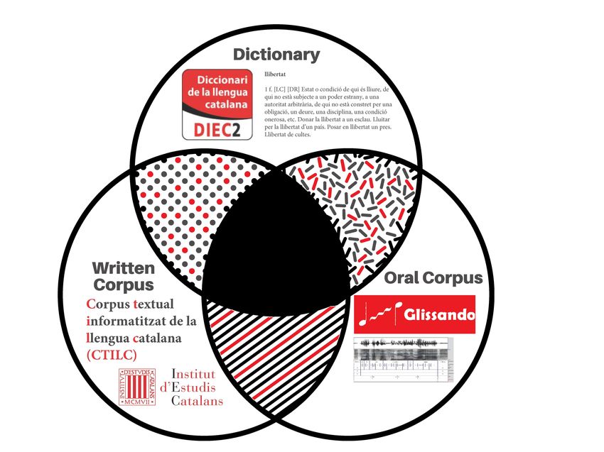
meanings of each word. The situation is depicted in Figure 1, where the corpora (the
spoken corpus and written corpus) and the dictionary used in this work are displayed as
a Venn diagram.
Fig 1. Graphical representation of the different sources used. Venn diagram
where the sources used in the present study are displayed as a sets: the normative
dictionary of the Catalan language (DIEC2), providing the number of meanings of each
word; the written corpus CTILC, providing the basis for the descriptive dictionary and
the dictionary of word frequencies of Catalan; and the speech corpus Glissando, that is
not initially lemmatized, but that has been lemmatized here with FreeLing [35].
Our analysis of the relationship between the number of meanings of a lemma and its
frequency consists in combining information about the number of meanings from the
official dictionary of the Catalan language (Diccionari de la llengua catalana,
DIEC2 [34]) with two sources for the frequency: written language (Corpus Textual
Informatitzat de la Llengua Catalana, CTILC) and speech (Glissando Corpus). As
shown in Figure 1, we work with a subset of each corpus, that is defined by the
intersection of the study corpus (spoken or written) with the dictionary, which implies
necessarily a decrease in the number of lemmas with respect to the initial corpus.
Finally, the total number of different lemmas of each corpus is specified in Table 1. The
intersection of the CTILC corpus with DIEC2 yields 52, 578 lemmas, while the
intersection of the Glissando corpus with DIEC2 yields 3, 083 lemmas.
CTILC is manually lemmatized and annotated with Parts-of-Speech (PoS) tags and
July 2, 2021 5/21Corpus Tokens Lemmas Available (website link)
CTILC 52 million 167,079 https://ctilc.iec.cat/
Glissando 93,069 4,510 Glissando at ELRA catalog
DIEC2 — 70,170 https://dlc.iec.cat/
CTILC ∩ DIEC2 — 52,578 CTILC and DIEC2
Glissando ∩ DIEC2 — 3,083 Glissando and DIEC2
Table 1. Summary of the data. Number of tokens, different lemmas and
availability details of the different sources used in the present study. The lemmas of the
Glissando corpus were obtained after lemmatization with Freeling [35]. For the DIEC2
dictionary, and its intersection with the respective corpora, the number of tokens is not
applicable because the dictionary only includes lemmas.
Glissando contains the direct transcriptions of spoken dialogues. In order to be able to
perform the same analysis in both corpora, we resorted to FreeLing1 to lemmatize the
Glissando corpus [35]. FreeLing is an open-source library offering a variety of linguistic
analysis functionalities for more than 12 languages, including Catalan. More specifically,
the natural language processing layers used in this work were:
Tokenization & sentence splitting: Given a text, split the basic lexical terms
(words, punctuation signs, numbers, etc.), and group these tokens into sentences.
Morphological analysis: Find out all possible Parts-of-Speech (PoS) for each token.
PoS-Tagging and Lemmatization: Determine the right PoS for each word in its
context. Determining the right PoS allows inferring the right lemma in almost all
cases.
Named Entity Recognition: Detect proper nouns in the text, which may be formed
by one or more tokens. We used only pattern-matching based detection relying
mainly on capitalization.
We used FreeLing [35] to perform PoS-tagging, lemmatization, and proper noun
detection on Glissando corpus. We then filtered out all tokens marked as punctuation,
number, or proper noun, before proceeding to count occurrences of each lemma and
cross them with DIEC2.
Of the 93, 069 tokens remaining after the filtering, 82, 838 (89%) were lemmatized by
FreeLing, producing 4, 510 different lemmas. The remaining 11% tokens correspond to
interjections, hesitations, half-words, foreign words (Spanish or English), colloquial
expressions, non-capitalized proper nouns, or transcription errors (where the
transcription was made phonetically, and not with the right form of the intended word)
and were left out of the study.
Fitting method
After intersecting each corpus with DIEC2 (Figure 1), we analized the resulting data
sets and fitted the power law functions of the three Zipfian laws, using linear Least
Squares (LS) on a logarithmic transoformation of both axes: the rank-frequency law,
the law of meaning distribution and the meaning-frequency law, as defined in Eq. 3,
Eq. 2 and Eq. 1, respectively.
Following Baayen’s method [39], we calculated the most likely breakpoint, i∗ (the
data point where the two regimes cross) in both corpora. The method consists of
scanning all possible breakpoints and compute, for each, the deviation (sum of squared
errors) or deviance, as Baayen’s refers to it, between the real points and Eq. 5. This
1 http://nlp.cs.upc.edu/freeling
July 2, 2021 6/21breakpoint is the rank that minimizes the deviance. Some care is required in this
method because there might be more than one local optimum, as we will see.
Since we are studying three interrelated Zipfian laws (rank-frequency law, law of
meaning distribution and meaning-frequency law), we decided, for simplicity, to transfer
the breakpoint obtained for the rank-frequency law to the other double regime laws.
The translation of the breakpoint to the double regime law of meaning distribution (Eq.
6) is immediate: the breakpoint, i∗ , is the same as in the rank-frequency law. The
translation of the i∗ to the breakpoint of the double regime meaning-frequency law (Eq.
7) requires computing f (i∗ ). The value of f (i∗ ) is calculated from the mean of the
frequencies of the data in the bin where i∗ is located. i∗ and f (i∗ ) are used to complete
the fitting and retrieve the exponents of the double regime laws. Accordingly, for the law
of meaning distribution, we fit Eq. 6, where the relevant parameters are γ1 and γ2 . For
the meaning frequency law, we fit Eq. 7 where the relevant parameters are δ1 and δ2 .
Curve smoothing
The fitting method described above is applied to two kinds of data: the raw data and
the smoothed data. In the raw data approach, every point of the curve corresponds to a
“word”. No bucketing or binning was applied. The smoothed data approach follows from
Zipf, who applied a linear binning technique to reduce noise in his analysis of the law of
meaning distribution [3, 5]. In previous work [13], Zipf’s analysis of the law in
English [3] was revisited and values for exponents very close to those already obtained
by Zipf were retrieved but, surprisingly, with sources of data differing from Zipf’s work:
in the case of the law of meaning distribution, γ achieving a value of 0.5 as in Zipf’s
pioneering research [5].
Given the robustness of this method, the data smoothing approach consisted of
estimating the exponents of the three Zipfian laws after applying a linear binning on the
data sets. In particular, we applied equal-size binning (K bins, each with n/K data
points), in the sense of having the same number of data points in each bin, considering n
the total number of lemmas of each subcorpus studied (Table 1). In equal-size binning,
resulting bins have an equal number of observations in each group. Bin sizes have been
chosen from divisors of the number of data points (lemmas) in each corpus to warrant
that every bin has the same number of points and that no data point is lost. CTILC ∩
DIEC2 contains 53, 578 lemmas and Glissando ∩ DIEC2 contains 3, 083 lemmas.
Results
One regime analysis
Fig. 2 and 3 show Zipf’s rank-frequency law for the CTILC corpus and the Glissando
corpus, respectively. Similarly, Fig. 4 and 5 show the meaning distribution law for
CTILC and Glissando, respectively, and Fig. 6 and 7 show the meaning-frequency law
for CTILC and Glissando, respectively. The values of the exponents of each law are
summarized in Table 2, both in the case of equal-size binning and also when no
smoothing is performed. Interestingly, γ approaches 0.5 in CTILC as the bin size
increases and the difference between δ and δ 0 (the predicted value of δ from α and γ in
Eq. 4), is slightly reduced when binning is used in both corpora.
Two regime analysis
After visual inspection of the rank-frequency law (Fig. 2 and 3), the appearance of at
least two regimes, i.e. straight lines in log-log scale with different slopes, is suggested in
the CTILC written corpus (Fig. 2). That is a well-known feature arising in large
July 2, 2021 7/21Fig 2. Zipf’s rank-frequency law in CTILC Corpus. Average frequency (f ) as a
function of rank (i) after applying equal-size binning (blue). The best fit of a power law
is also shown (red). Left: bin size of 127 words. Center: bins size of 414 words. Right:
bin size of 762 words.
Fig 3. Zipf’s rank-frequency law in Glissando Corpus. Average frequency (f )
as a function of rank (i) after applying equal-size binning (blue). The best fit of a power
law is also shown (red). Left: bin size of 23 words. Center: bins size of 46 words. Right:
bin size of 67 words.
Fig 4. Zipf’s law of meaning distribution in CTILC corpus. Average number
of meanings (µ) as a function of frequency rank (i) after applying equal-size binning
(blue). The best fit of a power law is also shown (red). Left: bin size of 127 words.
Center: bin size of 414 words. Right: bin size of 762 words. Sources: Catalan words in
CTILC, using DIEC2 meanings and CTILC frequencies.
multi-author corpora [16–18, 31–33]. However, interestingly, these two regimes are
apparently not visually observed in the Glissando speech corpus (Fig. 3) but they might
July 2, 2021 8/21Fig 5. Zipf’s law of meaning distribution in Glissando corpus. Average
number of meanings (µ) as a function of frequency rank (i) after applying equal-size
binning (blue). The best fit of a power law is also shown (red). Left: bin size of 23
words. Center: bin-size of 46 words. Right: bin-size of 67 words. Sources: Catalan
words in Glissando, using DIEC2 meanings and Glissando frequencies.
Fig 6. Zipf’s meaning-frequency law in CTILC corpus. Average number of
meanings (µ) as a function of frequency (f ) after applying equal-size binning (blue).
The best fit of a power law is also shown (red). Left: bin size of 127 words. Center: bin
size of 414 words. Right: bin size of 762 words. Sources: Catalan words in CTILC,
using DIEC2 meanings and CTILC frequencies.
Fig 7. Zipf’s meaning-frequency law in Glissando corpus. Average number of
meanings (µ) as a function of frequency (f ) after applying equal-size binning (blue).
The best fit of a power law is also shown (red). Left: bin size of 23 words. Center:
bin-size of 46 words. Right: bin-size of 67 words. Sources: Catalan words in Glissando,
using DIEC2 meanings and Glissando frequencies.
be hidden in the greater dispersion of the points in meaning distribution, despite the
linear binning, that can be seen in the speech corpus (Fig. 5) with respect to CTILC
July 2, 2021 9/21Binning Corpus bin size α γ δ δ0
No binning CTILC ∩ DIEC2 - 2.199 0.388 0.154 0.176
Glissando ∩ DIEC2 - 1.459 0.261 0.184 0.178
Equal-size CTILC ∩ DIEC2 127 2.228 0.471 0.187 0.211
414 2.286 0.478 0.187 0.209
762 2.347 0.484 0.187 0.206
Glissando ∩ DIEC2 23 1.483 0.304 0.210 0.205
46 1.513 0.306 0.206 0.202
67 1.542 0.312 0.205 0.202
Table 2. One regime analysis (CTILC and Glissando corpora). The exponents
of the Zipfian laws: the rank-frequency law (α, Eq. 3), the law of meaning distribution
(γ, Eq. 2) and meaning-frequency law (δ, Eq. 1). δ 0 is the exponent δ predicted by Eq. 4,
obtained from α and γ. For estimating the values of the parameters, we have used Least
Squares (LS) on a logarithmic transformation of both axes. Concerning equal-size
binning, see the Methods section for the rationale behind the choice of the bin sizes.
(Fig. 4).
To confirm the presence of two regimes in the CTILC corpus and shed light on the
possible presence of two regimes in the Glissando corpus, we perform a careful analysis
using Baayen’s method of breakpoint detection [39]. As can be seen in Fig. 8, the
deviance has only a single minimum in the case of CTILC corpus, which allows to
determine a breakpoint easily. Besides, a global minimum and a and and additional
local minimum are found in the Glissando corpus (Fig. 9): in the first binning (23 words
per bin), the global minimum does correspond to a meaningful two-regime breakpoint
but, in the other two binnings (46 and 67 words per bin), the global mininum
corresponds to a spurious result due to the abundance of hapax legomena in the tail of
the rank distribution, a phenomenon that can also be observed in the first binning
(Fig. 9). This spurious minimum in deviance can be explained by an artifact of the
deviance minimization procedure for breakpoint detection, that becomes too sensitive to
the concentration of points in the tail and the scarcity of points in other parts of the
curve when bin size increases [39]. As a result it is observed that when bin size
increases, the local minima in deviance decreases (see right panels in Fig. 9).
July 2, 2021 10/21104.314
104.314
105 40
104
30
frequency
deviance
103
A
20
102
101 10
100
102 103 104 102 103 104
rank rank
105 12
104.345
104.345
10
104
8
frequency
103
deviance
B 6
102
4
101
2
100
103 104 103 104
rank rank
105
104.366
104.366
5
104
4
103
frequency
deviance
C 3
102
2
101
1
100
103 104 103 104
rank rank
Fig 8. Breakpoint analysis for Zipf’s rank-frequency law in CTILC corpus.
Breakpoints (i∗ ) are depicted as blue dashed lines. Left: frequency (f ) as a function of
rank (i). The best fit of a two-regime power law is also shown (red). Right: Baayen’s
deviance as a function of rank (i). The choice of the bin sizes is the same as in Table 3
and influences the breakpoint. Row A) 127 words per bin and breakpoint 20, 606, row
B) 414 words per bin and breakpoint 22, 149, and row C) 762 words per bin and
breakpoint 23, 241.
July 2, 2021 11/210.80
102.523
103.397
102.523
103.397
103
0.75
102
frequency
deviance
A 0.70
101
0.65
100
101 102 103 101 102 103
rank rank
0.32
102.640
103.391
103
102.640
103.391
0.30
102
frequency
deviance
B 0.28
101
0.26
100 0.24
102 103 102 103
rank rank
103 0.22
102.701
103.388
102.701
103.388
0.20
102
frequency
deviance
C 0.18
101
0.16
100
102 103 102 103
rank rank
Fig 9. Breakpoint analysis for Zipf’s rank-frequency law in Glissando
corpus. Blue dashed lines and gray dashed lines are used to indicate, respectively, the
first and the second local minimum of deviance. The 1st local minimum is taken as the
meaningful breakpoint (i∗ ). Left: frequency (f ) as a function of rank (i). The best fit of
a two-regime power law is also shown (red). Right: Baayen’s deviance as a function of
rank (i). The choice of the bin sizes is the same as in Table 3 and influences the first
non-spurious breakpoint. Row A) 23 words per bin and breakpoint 333.5, row B) 46
words per bin and breakpoint 437.0, and row C) 67 words per bin and breakpoint 502.5.
The value of the breakpoint increases with the size of the bin. This value is
approximately 20, 606 (127 words per bin), 22, 149 (414 words per bin) and 23, 241 (762
words per bin) in the CTILC corpus (Fig. 8). In the Glissando corpus (Fig. 9), the
July 2, 2021 12/21non-spurious breakpoint is found at 333, 5 (23 words per bin), 437, 0 (46 words per bin)
and 502, 5 (67 words per bin). Evidently, the size of the corpus influences the the values
of these breakpoints.
Figure 10 shows the meaning-frequency law with this two regime analysis in CTILC
and Glissando corpora, and Figure 11 shows the two-regime in law of meaning
distribution. In both cases, by varying the bin size, the fitting curve for the CTILC
corpus has a clear breakpoint that divides the two regimes, while for the Glissando
corpus this breakpoint is not so clear visually, as there is greater dispersion of data in
the speech corpus and, consequently, a weaker correlation.
A
B
Fig 10. The meaning-frequency law in the CTILC and Glissando corpora.
Row A) CTILC corpus and row B) Glissando corpus. The choice of the bin sizes is the
same as in Table 3. Breakpoints (i∗ ) are depicted as dashed blue lines.
Table 3 summarizes the exponents of the Zipfian laws obtained in each of the two
regimes for the CTILC and Glissando corpora. The difference between δ1 and its
predicted value δ10 from Eq. 8, and the difference between δ2 and its predicted value δ20
from Eq. 9, are, in general, smaller than when a single regime was assumed in Table 2,
providing support for the reality of two-regime structure.
Discussion
Zipf’s laws of meaning and robustness of the equation between
exponents
Zipf’s laws of meaning have been verified in Catalan. Assuming a single regime and
applying equal-size binning to the CTILC corpus, the γ exponent of the law of meaning
distribution that Zipf found for the word meaning distribution law in English [3, 5] was
recovered approximately, γ ≈ 1/2, (Table 2), consistently with previous work [6, 8]. This
is not the case of the Glissando speech corpus where γ ≈ 0.304 − 0.312. Nonetheless,
considering the results for the fitting of a single slope (γ) for the law of meaning
distribution, the γ values obtained here are consistent with previous works [13, 15] that
extended the fitting of this law to non-Indo-European languages [12]. As shown in
previous research, verified here again for Catalan, there is a certain variability in the
July 2, 2021 13/21A
B
Fig 11. The law of meaning distribution in the CTILC and Glissando
corpora. Row A) CTILC corpus and row B) Glissando corpus. The choice of the bin
sizes is the same as in Table 3. Breakpoints (i∗ ) are depicted as dashed blue lines.
CTILC
Binning bin α1 α2 γ1 γ2 δ1 δ10 δ2 δ20
size
No binning – 1.414 4.483 0.419 0.298 0.275 0.296 0.052 0.066
Equal-size 127 1.480 4.560 0.494 0.402 0.312 0.334 0.073 0.088
414 1.600 4.707 0.503 0.388 0.297 0.314 0.068 0.082
762 1.707 4.800 0.512 0.375 0.286 0.300 0.065 0.078
Glissando
No binning – 0.853 1.537 0.065 0.287 0.059 0.076 0.194 0.187
Equal-size 23 1.281 1.583 0.098 0.405 0.071 0.076 0.262 0.256
46 1.404 1.583 0.102 0.436 0.069 0.073 0.275 0.275
67 1.495 1.577 0.110 0.459 0.072 0.074 0.291 0.291
Table 3. Two regime analysis (CTILC and Glissando corpora). The
exponents of each regime of the Zipfian laws: the rank-frequency law (α1 and α2 ), the
law of meaning distribution (γ1 and γ2 ) and meaning-frequency law (δ1 and δ2 ). δ10 is
the exponent δ1 predicted by Eq. 9 while δ20 is the exponent δ2 predicted by Eq. 8. To
obtain the exponents, we used LS following Baayen’s method [39]. Concerning
equal-size binning, see the Methods section for the rationale behind the choice of the bin
sizes. Subindexes of the exponents correspond to the regimes according to Eq. 5, Eq. 6
and Eq. 7.
exponents of the Zipfian laws according to the size of the binning [12, 13, 15].
However, there were clear deviations in Zipf’s rank-frequency law exponent, i.e. α,
with respect to Catalan (α = 1.42 in [29] using different methods) and other languages
in normal conditions [40, 41]. Consequently, this fact affected the exponent δ 0 obtained
indirectly with Eq. 4 (see Table 2). These considerations notwithstanding, δ 0 gives
approximately a similar value as the δ obtained directly from the meaning-frequency
law (δ 0 = 0.187 − 0.21 (CTILC corpus) and δ 0 = 0.20 − 0.21 (Glissando corpus)) but
deviates in both cases from the previously estimated for English [5, 6]. The well-known
deviations in Zipf’s rank-frequency law (Eq. 3) imply that it cannot be assumed that
July 2, 2021 14/21α = 1 in general [40, 41], therefore, according to Eq. 4, it cannot be expected that γ = δ
as in Zipf’s early work [5, 12].
Nevertheless, the Equation 4 to obtain δ 0 indirectly is even robust in the case of the
analysis of one regime without binning in both corpus (Table 2). This is especially
interesting given that, in this case, both in the CTILC corpus (α ≈ 2.20, γ ≈ 0.39) and
in Glissando (α ≈ 1.46, γ ≈ 0.26) the Zipfian exponents are far from the usual ones but
δ ≈ δ 0 . On the other hand, the minimal differences found in α with respect to the
previous study of the Glissando corpus [29] (where α ≈ 1.42) may be due to the fact
that here we have worked with a subcorpus of Glissando (Glissando ∩ DIEC2) and with
different methods.
On the other hand, after verifying the existence of two regimes in Zipf’s
rank-frequency law in CTILC corpus (Fig. 2 and 8) and in Glissando corpus (Fig. 3 and
9), as previous works pointed out in big corpora [16, 18, 31], we have seen that this
affects the meaning-frequency law (Fig. 10). Then, the analysis of the two regimes in
the CTILC corpus allowed us to obtain in the first regime γ1 ≈ 1/2 and δ1 ≈ 0.30 (with
δ1 ≈ δ10 ), and in the second regime γ2 = 0.37 − 0.40 and δ2 ≈ 0.06 − 0.07 (and again
δ20 ≈ 0.08). In the case of the Glissando corpus in the first regime (binning size 23)
γ1 ≈ 0.1 and δ1 ≈ 0.07 (with δ1 ≈ δ10 ), and in the second regime γ2 = 0.405 and
δ2 ≈ 0.26, and again δ2 ≈ δ20 . Results are similar for other bin sizes, as can be seen in
Table 3.
Finally, our experimental results show that the relationship (Eq. 4) between the
three Zipfian exponents [6, 8] is specially robust when we two regimes are assumed as
expected from the higher precision in the estimation of the exponents. Again, δ and δ 0
deviate from previously reported for English, δ ≈ 0.5 [5, 6, 8]. δ 0 may deviate from the
expected value because of the value of α retrieved here for Catalan. Besides, δ may
deviate from the expected value because of the two regime structure of the data.
Therefore, as a hypothesis to corroborate in future research employing more languages,
the variations in γ or δ could be explained by deviations in Zipf’s rank-frequency law or
the underlying two regime structure reported here.
Two regimes in Zipfian laws: core vocabulary?
In sum, although we have verified Zipf’s meaning-frequency law (Eq. 1) between the
number of meanings and the frequency of words in Catalan employing Zipf’s binning
technique [5], data is better-described when two regimes are assumed. These two scaling
regimes could be explained simply as the outcome of aggregating texts: previous work
indicate that scaling breaks in rank-frequency distributions are a consequence of the
mixing and composition of texts and corpora [18].
Previous works showed that some variability was found in the breakpoints in the
case of corpus of English, Spanish and Portuguese, depending on the size of the
corpus [18]. Here, for both corpora, we have seen that the breakpoint tends to increase
with the size of the corpus and also with the size of the bin, and in the case of CTILC
corpus (167, 079 lemmas) the breakpoint varies from 20, 606 to 23, 241, and in Glissando
corpus (4510 lemmas) from 333.5 to 502.5. Therefore, in the case of Catalan we have
also seen this dependence with the size of the corpus.
In our opinion, as seen, the effects of corpus size, composition and heterogeneity
previously suggested [17, 18, 40, 42] are not incompatible with the existence of a core and
a peripheral vocabulary or ”unlimited lexicon” [16, 33], but this dichotomy is not
necessarily be an observable property of Zipfian distributions by means of the
breakpoint as [18] pointed out. Besides, if we understand the core vocabulary as the
real basic vocabulary of a linguistic community at a given time, then Glissando turns
out to be a better source than CTILC to capture that subset of the vocabulary, because
CTILC corpus mixed sources from different time periods.
July 2, 2021 15/21One the one hand, the CTILC written corpus includes from literary and journalistic
texts to scientific ones, in a time interval of more than a century, with the diachronic
variations that this implies. The sum of the size effect and the greater linguistic
variability of combining heterogeneous texts in the CTILC corpus could explain the
appearance of two regimes in Zipf’s rank-frequency law [17, 18, 32] and, as we have seen,
consequently, of two regimes in the Zipf’s meaning-frequency law. On the other hand,
Glissando is a synchronous speech corpus in which the interlocutors cooperate and
circumscribe themselves to a single communicative context, as is often promoted in the
systematic design of speech corpora [37]. That is, to the usual reduction in the use of
rare words that occurs in oral communication, in a pragmatic context with broad
Gricean implications (see [43] and [44] for a review), it must be added that in the
construction of speech corpus like Glissando, literally communicative scenarios are
’designed’ [37]. This fact causes that we are not really facing a spontaneous speech
corpus, causing a tendency to unify the vocabulary used by the different informants
involved in or, at least, reducing the use of infrequent words. Infrequent words are
typical of the peripheral vocabulary of multi-author corpus that deal with diverse topics.
However, in the speech corpus a greater dispersion of the points in the
meaning-frequency distribution is appreciated, but the two regimes are still found.
Lexical diversity is defined as the variety of vocabulary deployed in a text or
transcript by either a speaker or a writer [45]. In speech one expects to find a smaller
lexical diversity and core vocabulary given the stronger cognitive constraints of
spontaneous oral language (Glissando) with respect to written language (CTILC), to
which the effects of the lemmatization are added here (see next subsection). Size effects
have been shown to influence lexical diversity, even in small corpus [46].
Therefore, other speech corpora of different size and spontaneous speech should be
analysed in the future to corroborate these two regimes observed, exploring the size
limits that had previously been considered for the appearance of a kernel
vocabulary [16]. It also remains as future work to verify if these effects are present in
the comparison of spoken and written corpora of other languages and, in addition, if
these two regimes appear in other languages, analogously to Catalan, in multi-author
texts or whether they appear just as a consequence of text mixing [18, 31], given the
influence of semantics on Zipfian distributions [11, 47].
Lemmatization and binning effects
Glissando is a corpus smaller in size than CTILC and with less thematic variability.
However, the effect of binning seems to be added to the effect of corpus size. As Table 1
shows, only the lemmas for which we had their meanings have been analyzed
(intersection of each corpus with the DIEC2 dictionary). Thus, there is eventually an
order of magnitude difference between the number of lemmas in both corpora (the
intersection of CTILC corpus with DIEC2 has 52, 578 lemmas and the intersection of
Glissando corpus with DIEC2 only 3, 083 lemmas). The quantitative effects of corpus
size have been related to variations of Zipf’s law and other linguistic laws in such a way
that a larger size in a corpus implies increasing the probability of rare words, so that
word frequency distributions are Large Number of Rare Events (LNRE) as [42] explain
clearly. Thus, in the case of the speech corpus such as Glissando, smaller in size, also
there is a smaller number of rare words, since fewer technical words and jargon are used
in orality than in written corpus [48], but the two regimes are nevertheless observed.
The lemmatization process implies a decrease in the LNRE by including under the same
lemma inflected words, of special importance in Catalan [36], as in other Romance
languages [21, 26].
Regarding the deviations observed in the exponents of Zipf’s rank-frequency law
(Eq. 3) also found in other languages [49], notice that by lemmatizing the corpus the
July 2, 2021 16/21morphological complexity and, by extension, the diversity of the vocabulary, is reduced.
As explained in the introduction, Catalan is a Romance language with a rich inflection
and derivation [21, 25, 27], that, however, it does not stand out typologically compared
to other languages in terms of indicators of entropy rate or phonological and
morphological richness [22–24].
The robustness of Zipf’s law under lemmatization for single-author written texts was
already checked in previous work studying Spanish, French and English with different
methods [50]. The exponent of lemmas and word forms may vary but both are
correlated in texts [50] and the same could happen in speech corpora. However, one
could consider an opposite hypotheses that should be confirmed in future works,
including more languages: that the lemmatization, as a source of reduction of
morphological richness, should vary the exponent of Zipf’s rank-frequency law [50], and
this variation would depend on the inflectional and derivational complexity of the
language (in the sense of Bentz’s works [22–24]), that is, it will affect the languages with
more morphological variability to a greater extent.
Following [51] the α exponent of Zipf’s rank-frequency law ”reflects changes in
morphological marking” [51], so that more inflection is correlated to a higher α and
longer tail of hapax legomena [22, 51]. Comparing modalities, in our case orality shows a
lower α than writing, contrary to [51] but consider that here we follow different
methods. Besides, it has been shown that there is variability in α related to both the
text genre and the linguistic typology for languages of different linguistic families [49].
Future research should control for both effects (modality and morphological complexity)
with corpora that are closer and employing uniform methods.
Future work should clarify how factors such as corpus size, binning and linguistic
variability, influence Zipf’s meaning-frequency law. The relationship between the
exponents of the laws confirmed here for Catalan should be investigated for other
languages. Our findings call for a revision of previous research of these laws assuming
one regime.
Acknowledgements
We are grateful to C. Bentz, J. M. Garrido, C. Santamaria, J. Rafel and the technicians
of Oficines Lexicogràfiques de l’Institut d’Estudis Catalans (Institute of Catalan
Studies) for providing us with the data and helpful comments. This work has been
funded by the projects PRO2020-S03 (RCO03080 Lingüı́stica Quantitativa) and
PRO2021-S03 HERNANDEZ from Institut d’Estudis Catalans. JB, RFC and AHF are
also funded by the grant TIN2017-89244-R from Ministerio de Economia, Industria y
Competitividad (Gobierno de España) and supported by the recognition 2017SGR-856
(MACDA) from AGAUR (Generalitat de Catalunya).
References
1. G. K. Zipf, Selected studies of the principle of relative frequency in language,
Harvard University Press, 1932.
2. G. K. Zipf, The Psychobiology of Language, an Introduction to Dynamic
Philology, Houghton–Mifflin, Boston, 1935.
3. G. K. Zipf, Human Behavior and the Principle of Least Effort, Addison–Wesley,
Cambridge, MA, 1949.
July 2, 2021 17/214. I. G. Torre, B. Luque, L. Lacasa, C. T. Kello, A. Hernández-Fernández, On the
physical origin of linguistic laws and lognormality in speech, Royal Society Open
Science 6 (2019) 191023. doi:10.1098/rsos.191023.
5. G. K. Zipf, The meaning-frequency relationship of words, Journal of General
Psychology 33 (1945) 251–256. doi:10.1080/00221309.1945.10544509.
6. R. Ferrer-i-Cancho, M. Vitevitch, The origins of Zipf’s meaning-frequency law,
Journal of the American Association for Information Science and Technology 69
(2018) 1369–1379. doi:/10.1002/asi.24057.
7. R. H. Baayen, F. M. del Prado Martı́n, Semantic density and past-tense
formation in three Germanic languages, Language 81 (2005) 666–698. URL:
http://www.jstor.org/stable/4489969.
8. R. Ferrer-i-Cancho, The optimality of attaching unlinked labels to unlinked
meanings, Glottometrics 36 (2016) 1–16. URL:
http://hdl.handle.net/2117/102539.
9. A. Hernandez Fernandez, R. Ferrer-i-Cancho, Lingüı́stica cuantitativa: la
estadı́stica de las palabras, EMSE EDAPP / Prisanoticias, 2019. URL:
https://colecciones.elpais.com/literatura/
118-grandes-ideas-de-las-matematicas.html.
10. E. U. Condon, Statistics of vocabulary, Science 67 (1928) 300.
11. D. Carrera-Casado, R. F. i Cancho, The advent and fall of a vocabulary learning
bias from communicative efficiency, https://arxiv.org/abs/2105.11519 (2021).
12. F. Bond, A. Janz, M. Maziarz, E. Rudnicka, Testing Zipf’s meaning-frequency
law with wordnets as sense inventories, in: Wordnet Conference, 2019, p. 342.
13. B. Casas, A. Hernández-Fernández, N. Català, R. Ferrer-i-Cancho, J. Baixeries,
Polysemy and brevity versus frequency in language, Computer Speech and
Language 58 (2019) 19 – 50. doi:10.1016/j.csl.2019.03.007.
14. A. Hernández-Fernández, B. Casas, R. Ferrer-i-Cancho, J. Baixeries, Testing the
robustness of laws of polysemy and brevity versus frequency, in: P. Král,
C. Martı́n-Vide (Eds.), Statistical Language and Speech Processing, Springer
International Publishing, Cham, 2016, pp. 19–29.
15. B. Ilgen, B. Karaoglan, Investigation of Zipf’s ‘law-of-meaning’ on Turkish
corpora, in: 22nd International Symposium on Computer and Information
Sciences, 2007, pp. 1–6. URL:
https://ieeexplore.ieee.org/document/4456846.
16. R. Ferrer-i-Cancho, R. Solé, Two regimes in the frequency of words and the
origins of complex lexicons: Zipf’s law revisited, Journal of Quantitative
Linguistics 8 (2001) 165–173.
17. M. A. Montemurro, Beyond the Zipf–Mandelbrot law in quantitative linguistics,
Physica A: Statistical Mechanics and its Applications 300 (2001) 567 – 578.
doi:https://doi.org/10.1016/S0378-4371(01)00355-7.
18. J. R. Williams, J. P. Bagrow, C. M. Danforth, P. S. Dodds, Text mixing shapes
the anatomy of rank-frequency distributions, Phys. Rev. E 91 (2015) 052811.
doi:10.1103/PhysRevE.91.052811.
July 2, 2021 18/2119. B. Mandelbrot, Information theory and psycholinguistics: A theory of word
frequencies, in: P. F. Lazarsfield, N. Henry (Eds.), Readings in mathematical
social sciences, Cambridge: MIT Press, 1966, pp. 550–562.
20. W. Li, P. Miramontes, G. Cocho, Fitting ranked linguistic data with
two-parameter functions, Entropy 12 (2010) 1743–1764.
21. J. Kabatek, C. D. Pusch, The Romance languages, in: B. Kortmann, J. Van der
Auwera (Eds.), The languages and linguistics of Europe: A comprehensive guide,
volume 1, Walter de Gruyter, Berlin, 2011, pp. 69–96.
22. C. Bentz, Adaptive languages: An information-theoretic account of linguistic
diversity, volume 316, Walter de Gruyter GmbH & Co KG, 2018.
23. C. Bentz, D. Alikaniotis, M. Cysouw, R. Ferrer-i-Cancho, The entropy of
words—learnability and expressivity across more than 1000 languages, Entropy
19 (2017). URL: https://www.mdpi.com/1099-4300/19/6/275.
doi:10.3390/e19060275.
24. C. Bentz, T. Ruzsics, A. Koplenig, T. Samardžić, A comparison between
morphological complexity measures: Typological data vs. language corpora, in:
Proceedings of the Workshop on Computational Linguistics for Linguistic
Complexity (CL4LC), The COLING 2016 Organizing Committee, Osaka, Japan,
2016, pp. 142–153. URL: https://www.aclweb.org/anthology/W16-4117.
25. E. Clua Julve, Gènere i nombre en els noms i en els adjectius, in: J. Solà, M. R.
Lloret, J. Mascaró, M. P. Saldanya (Eds.), Gramàtica del català contemporani
(1), Editorial Empúries, Barcelona, 2002, pp. 485–534.
26. F. Montermini, The lexical representation of nouns and adjectives in Romance
languages, Recherches linguistiques de Vincennes 39 (2010) 135–162. URL:
http://journals.openedition.org/rlv/1869. doi:10.4000/rlv.1869.
27. O. Domènech, R. Estopà, La neologia per sufixació: anàlisi contrastiva entre
varietats diatòpiques de la llengua catalana, Caplletra. Revista Internacional de
Filologia 51 (2011) 9–33.
28. R. Köhler, G. Altmann, R. G. Piotrowski, Quantitative Linguistik/Quantitative
Linguistics: ein internationales Handbuch/an international handbook, volume 27,
Walter de Gruyter, 2008.
29. A. Hernández-Fernández, I. González-Torre, J. Garrido, L. Lacasa, Linguistic
laws in speech: the case of Catalan and Spanish, Entropy 21 (2019)
e21121153:1–e21121153:16. doi:10.3390/e21121153.
30. A. Corral, I. Serra, The brevity law as a scaling law, and a possible origin of
Zipf’s law for word frequencies, Entropy 22 (2020). doi:10.3390/e22020224.
31. A. M. Petersen, J. N. Tenenbaum, S. Havlin, H. E. Stanley, M. Perc, Languages
cool as they expand: Allometric scaling and the decreasing need for new words,
Scientific reports 2 (2012) 943.
32. M. A. Montemurro, D. H. Zanette, New perspectives on Zipf’s law in linguistics:
from single texts to large corpora, Glottometrics 4 (2002) 87–99.
33. M. Gerlach, E. G. Altmann, Stochastic model for the vocabulary growth in
natural languages, Phys. Rev. X 3 (2013) 021006.
doi:10.1103/PhysRevX.3.021006.
July 2, 2021 19/2134. I. Institut d’Estudis Catalans, Diccionari de la llengua catalana, Edicions 62:
Enciclopèdia Catalana [1st ed. 1995], on line version in: http://dcc.iec.cat, 2020.
35. L. Padró, E. Stanilovsky, Freeling 3.0: Towards wider multilinguality, in:
Proceedings of the Eight International Conference on Language Resources and
Evaluation (LREC), 2012, pp. 2473–2479. URL:
http://www.lrec-conf.org/proceedings/lrec2012/summaries/430.html.
36. J. Rafel i Fontanals, Diccionari de freqüències, volume 3, Institut d’Estudis
Catalans, Barcelona, 1998.
37. J. M. Garrido, D. Escudero, L. Aguila, V. Cardeñoso, E. Rodero, C. de-la Mota,
C. González, S. Rustullet, O. Larrea, Y. Laplaza, F. Vizcaı́no, M. Cabrera,
A. Bonafonte, Glissando: a corpus for multidisciplinary prosodic studies in
Spanish and Catalan, Language Resources and Evaluation 47 (2013) 945–971.
38. C. D. Manning, P. Raghavan, H. Schütze, Introduction to information retrieval,
volume 20, Cambridge University Press, 2008.
39. H. Baayen, Analyzing linguistic data: A practical introduction to statistics using
R, Cambridge University Press, 2008.
40. R. Ferrer-i-Cancho, The variation of Zipf’s law in human language, The European
Physical Journal B-Condensed Matter and Complex Systems 44 (2005) 249–257.
41. J. Baixeries, B. Elvevåg, R. Ferrer-i-Cancho, The evolution of the exponent of
Zipf’s law in language ontogeny, PLOS ONE 8 (2013) 1–14.
doi:10.1371/journal.pone.0053227.
42. R. Baayen, Word Frequency Distributions, Text, Speech and Language
Technology, Springer Netherlands, 2001. URL:
https://books.google.es/books?id=FWicxYWJP9sC.
43. H. P. Grice, Logic and conversation, in: Speech acts, Brill, 1975, pp. 41–58.
44. B. L. Davies, Grice’s cooperative principle: Meaning and rationality, Journal of
Pragmatics 39 (2007) 2308 – 2331.
doi:https://doi.org/10.1016/j.pragma.2007.09.002.
45. P. M. McCarthy, S. Jarvis, Mtld, vocd-d, and hd-d: A validation study of
sophisticated approaches to lexical diversity assessment, Behavior research
methods 42 (2010) 381–392.
46. R. Koizumi, Y. In’nami, Effects of text length on lexical diversity measures:
Using short texts with less than 200 tokens, System 40 (2012) 554–564.
47. S. T. Piantadosi, Zipf’s word frequency law in natural language: A critical review
and future directions, Psychonomic Bulletin & Review 21 (2014) 1112–1130.
48. V. Johansson, Lexical diversity and lexical density in speech and writing, Lund
University, Department of Linguistics and Phonetics (2008).
49. S. Yu, C. Xu, H. Liu, Zipf’s law in 50 languages: its structural pattern, linguistic
interpretation, and cognitive motivation, 2018. arXiv:1807.01855.
50. A. Corral, G. Boleda, R. Ferrer-i-Cancho, Zipf’s law for word frequencies: Word
forms versus lemmas in long texts, PLOS ONE 10 (2015) 1–23.
doi:10.1371/journal.pone.0129031.
July 2, 2021 20/2151. V. Chand, D. Kapper, S. Mondal, S. Sur, R. D. Parshad, Indian English
evolution and focusing visible through power laws, Languages 2 (2017). URL:
https://www.mdpi.com/2226-471X/2/4/26. doi:10.3390/languages2040026.
July 2, 2021 21/21You can also read