DEVISE: A DEEP VISUAL-SEMANTIC EMBEDDING MODEL
←
→
Page content transcription
If your browser does not render page correctly, please read the page content below

DeViSE: A Deep Visual-Semantic Embedding Model

                   Andrea Frome*, Greg S. Corrado*, Jonathon Shlens*, Samy Bengio
                         Jeffrey Dean, Marc’Aurelio Ranzato, Tomas Mikolov
                                    * These authors contributed equally.

    {afrome, gcorrado, shlens, bengio, jeff, ranzato†, tmikolov}@google.com
                                                   Google, Inc.
                                              Mountain View, CA, USA

                                                    Abstract
             Modern visual recognition systems are often limited in their ability to scale to
             large numbers of object categories. This limitation is in part due to the increasing
             difficulty of acquiring sufficient training data in the form of labeled images as the
             number of object categories grows. One remedy is to leverage data from other
             sources – such as text data – both to train visual models and to constrain their pre-
             dictions. In this paper we present a new deep visual-semantic embedding model
             trained to identify visual objects using both labeled image data as well as seman-
             tic information gleaned from unannotated text. We demonstrate that this model
             matches state-of-the-art performance on the 1000-class ImageNet object recogni-
             tion challenge while making more semantically reasonable errors, and also show
             that the semantic information can be exploited to make predictions about tens
             of thousands of image labels not observed during training. Semantic knowledge
             improves such zero-shot predictions achieving hit rates of up to 18% across thou-
             sands of novel labels never seen by the visual model.

1       Introduction
The visual world is populated with a vast number of objects, the most appropriate labeling of which
is often ambiguous, task specific, or admits multiple equally correct answers. Yet state-of-the-
art vision systems attempt to solve recognition tasks by artificially assigning images to a small
number of rigidly defined classes. This has led to building labeled image data sets according to
these artificial categories and in turn to building visual recognition systems based on N-way discrete
classifiers. While growing the number of labels and labeled images has improved the utility of
visual recognition systems [7], scaling such systems beyond a limited number of discrete categories
remains an unsolved problem. This problem is exacerbated by the fact that N-way discrete classifiers
treat all labels as disconnected and unrelated, resulting in visual recognition systems that cannot
transfer semantic information about learned labels to unseen words or phrases. One way of dealing
with this issue is to respect the natural continuity of visual space instead of artificially partitioning
it into disjoint categories [20].
We propose an approach that addresses these shortcomings by training a visual recognition model
with both labeled images and a comparatively large and independent dataset – semantic information
from unannotated text data. This deep visual-semantic embedding model (DeViSE) leverages textual
data to learn semantic relationships between labels, and explicitly maps images into a rich semantic
embedding space. We show that this model performs comparably to state-of-the-art visual object
classifiers when trained and evaluated on flat 1-of-N metrics, while simultaneously making fewer
semantically unreasonable mistakes along the way. Furthermore, we show that the model leverages
    †
        Current affiliation: Facebook, Inc.

                                                        1
visual and semantic similarity to correctly predict object category labels for unseen categories, i.e.
“zero-shot” classification, even when the number of unseen visual categories is 20,000 for a model
trained on just 1,000 categories.

2     Previous Work
The current state-of-the-art approach to image classification is a deep convolutional neural network
trained with a softmax output layer (i.e. multinomial logistic regression) that has as many units
as the number of classes (see, for instance [11]). However, as the number of classes grows, the
distinction between classes blurs, and it becomes increasingly difficult to obtain sufficient numbers
of training images for rare concepts.
One solution to this problem, termed WSABIE [20], is to train a joint embedding model of both im-
ages and labels, by employing an online learning-to-rank algorithm. The proposed model contained
two sets of parameters: (1) a linear mapping from image features to the joint embedding space, and
(2) an embedding vector for each possible label. Compared to the proposed approach, WSABIE
only explored linear mappings from image features to the embedding space, and the available labels
were only those provided in the image training set. It could thus not generalize to new classes.
More recently, Socher et al [18] presented a model for zero-shot learning where a deep neural
network was first trained in an unsupervised manner from many images in order to obtain a rich
image representation [3]; in parallel, a neural network language model [2] was trained in order to
obtain embedding representations for thousands of common terms. The authors trained a linear
mapping between the image representations and the word embeddings representing 8 classes for
which they had labeled images, thus linking the image representation space to the embedding space.
This last step was performed using a mean-squared error criterion. They also trained a simple model
to determine if a given image was from any of the 8 original classes or not (i.e., an outlier detector).
When the model determined an image to be in the set of 8 classes, a separately trained softmax
model was used to perform the 8-way classification; otherwise the model predicted the nearest class
in the embedding space (in their setting, only 2 outlier classes were considered). Their model differs
from our proposed approach in several ways: first and foremost, the scale, as our model considers
1,000 known classes for the image model and up to 20,000 unknown classes, instead of respectively
8 and 2; second, in [18] there is an inherent trade-off between the quality of predictions for trained
and outlier classes; third, by using a different visual model, different language model, and different
training objective, we were able to train a single unified model that uses only embeddings.
There has been other recent work showing impressive zero-shot performance on visual recognition
tasks [12, 17, 16], however all of these rely on a curated source of semantic information for the
labels: the WordNet hierarchy is used in [12] and [17], and [16] uses a knowledge base containing
descriptive properties for each class. By contrast, our approach learns its semantic representation
directly from unannotated data.

3     Proposed Approach
Our objective is to leverage semantic knowledge learned in the text domain, and transfer it to a model
trained for visual object recognition. We begin by pre-training a simple neural language model well-
suited for learning semantically-meaningful, dense vector representations of words [13]. In parallel,
we pre-train a state-of-the-art deep neural network for visual object recognition [11], complete with
a traditional softmax output layer. We then construct a deep visual-semantic model by taking the
lower layers of the pre-trained visual object recognition network and re-training them to predict the
vector representation of the image label text as learned by the language model. These three training
phases are detailed below.

3.1   Language Model Pre-training

The skip-gram text modeling architecture introduced by Mikolov et al [13, 14] has been shown to
efficiently learn semantically-meaningful floating point representations of terms from unannotated
text. The model learns to represent each term as a fixed length embedding vector by predicting
adjacent terms in the document (Figure 1a, right). We call these vector representations embedding

                                                   2
A                                                                                                        B
           Traditional                      Deep Visual Semantic                                Skip-gram
          Visual Model                       Embedding Model                                 Language Model
              label                               similarity metric                            nearby word

          softmax layer                    transformation
                                                                                               softmax layer

              core                              core          embedding                         embedding
             visual                            visual           vector                            vector
             model         parameter           model         lookup table    parameter         lookup table
                          initialization                                    initialization
                                                                                                                   reptiles
             image                             image             label                         source word         birds                 insects    food
                                                                                                                   musical instruments   clothing   dogs
                                                                                                                   aquatic life          animals    transportation

Figure 1: (a) Left: a visual object categorization network with a softmax output layer; Right: a skip-gram
language model; Center: our joint model, which is initialized with parameters pre-trained at the lower layers
of the other two models. (b) t-SNE visualization [19] of a subset of the ILSVRC 2012 1K label embeddings
learned using skip-gram.

vectors. Because synonyms tend to appear in similar contexts, this simple objective function drives
the model to learn similar embedding vectors for semantically related words.
We trained a skip-gram text model on a corpus of 5.7 million documents (5.4 billion words) extracted
from wikipedia.org. The text of the web pages was tokenized into a lexicon of roughly 155,000
single- and multi-word terms consisting of common English words and phrases as well as terms from
commonly used visual object recognition datasets [7]. Our skip-gram model used a hierarchical
softmax layer for predicting adjacent terms and was trained using a 20-word window with a single
pass through the corpus. For more details and a pointer to open-source code, see [13].
We trained skip-gram models of varying hidden dimensions, ranging from 100-D to 2,000-D, and
found 500- and 1,000-D embeddings to be a good compromise between training speed, semantic
quality, and the ultimate performance of the DeViSE model described below. The semantic quality
of the embedding representations learned by these models is impressive.1 A visualization of the lan-
guage embedding space over a subset of ImageNet labels indicates that the language model learned
a rich semantic structure that could be exploited in vision tasks (Figure 1b).

3.2   Visual Model Pre-training

The visual model architecture we employ is based on the winning model for the 1,000-class Ima-
geNet Large Scale Visual Recognition Challenge (ILSVRC) 2012 [11, 6]. The deep neural network
model consists of several convolutional filtering, local contrast normalization, and max-pooling lay-
ers, followed by several fully connected neural network layers trained using the dropout regular-
ization technique [10]. We trained this model with a softmax output layer, as described in [11], to
predict one of 1,000 object categories from the ILSVRC 2012 1K dataset [7], and were able to repro-
duce their results. This trained model serves both as our benchmark for performance comparisons,
as well as the initialization for our joint model.

3.3   Deep Visual-Semantic Embedding Model

Our deep visual-semantic embedding model (DeViSE) is initialized from these two pre-trained neu-
ral network models (Figure 1a). The embedding vectors learned by the language model are unit
normed and used to map label terms into target vector representations2 .
The core visual model, with its softmax prediction layer now removed, is trained to predict these
vectors for each image, by means of a projection layer and a similarity metric. The projection layer
is a linear transformation that maps the 4,096-D representation at the top of our core visual model
into the 500- or 1,000-D representation native to our language model.
   1
     For example, the 9 nearest terms to tiger shark using cosine distance are bull shark, blacktip shark, shark,
oceanic whitetip shark, sandbar shark, dusky shark, blue shark, requiem shark, and great white shark. The
9 nearest terms to car are cars, muscle car, sports car, compact car, automobile, racing car, pickup truck,
dealership, and sedans.
   2
     In [13], which introduced the skip-gram model for text, cosine similarity between vectors is used for
measuring semantic similarity. Unit-norming the vectors and using dot product similarity is an equivalent
similarity measurement.

                                                                                    3
The choice of loss function proved to be important. We used a combination of dot-product similarity
and hinge rank loss (similar to [20]) such that the model was trained to produce a higher dot-product
similarity between the visual model output and the vector representation of the correct label than be-
tween the visual output and other randomly chosen text terms. We defined the per training example
hinge rank loss:
                                 X
       loss(image, label) =            max[0, margin − ~tlabel M~v (image) + ~tj M~v (image)]      (1)
                                  j6=label

 where ~v (image) is a column vector denoting the output of the top layer of our core visual network
 for the given image, M is the matrix of trainable parameters in the linear transformation layer,
~tlabel is a row vector denoting learned embedding vector for the provided text label, and ~tj are
 the embeddings of other text terms. In practice, we found that it was expedient to randomize the
 algorithm both by (1) restricting the set of false text terms to possible image labels, and (2) truncating
 the sum after the first margin-violating false term was encountered. The ~t vectors were constrained
 to be unit norm, and a fixed margin of 0.1 was used in all experiments3 . We also experimented
 with an L2 loss between visual and label embeddings, as suggested by Socher et al. [18], but that
 consistently yielded about half the accuracy of the rank loss model. We believe this is because the
 nearest neighbor evaluation is fundamentally a ranking problem and is best solved with a ranking
 loss, whereas the L2 loss only aims to make the vectors close to one another but remains agnostic to
 incorrect labels that are closer to the target image.
The DeViSE model was trained by asynchronous stochastic gradient descent on a distributed com-
puting platform described in [4]. As above, the model was presented only with images drawn from
the ILSVRC 2012 1K training set, but now trained to predict the term strings as text4 . The param-
eters of the projection layer M were first trained while holding both the core visual model and the
text representation fixed. In the later stages of training the derivative of the loss function was back-
propagated into the core visual model to fine-tune its output5 , which typically improved accuracy
by 1-3% (absolute). Adagrad per-parameter dynamic learning rates were utilized to keep gradients
well scaled at the different layers of the network [9].
At test time, when a new image arrives, one first computes its vector representation using the visual
model and the transformation layer; then one needs to look for the nearest labels in the embedding
space. This last step can be done efficiently using either a tree or a hashing technique, in order to
be faster than the naive linear search approach (see for instance [1]). The nearest labels are then
mapped back to ImageNet synsets for scoring (see Section A.2 for details).

4       Results
The goals of this work are to develop a vision model that makes semantically relevant predictions
even when it makes errors and that generalizes to classes outside of its labeled training set, i.e. zero-
shot learning. We compare DeViSE to two models that employ the same high-quality core vision
model, but lack the semantic structure imparted by our language model: (1) a softmax baseline
model – a state-of-the-art vision model [11] which employs a 1000-way softmax classifier; (2) a
random embedding model – a version of our model that uses random unit-norm embedding vectors
in place of those learned by the language model. Both use the trained visual model described in
Section 3.2.
In order to demonstrate parity with the softmax baseline on the most commonly-reported metric, we
compute “flat” hit@k metrics – the percentage of test images for which the model returns the one
true label in its top k predictions. To measure the semantic quality of predictions beyond the true
label, we employ a hierarchical precision@k metric based on the label hierarchy provided with the
    3
      The margin was chosen to be a fraction of the norm of the vectors, which is 1.0. A wide range of values
would likely work well.
    4
      ImageNet image labels are synsets, a set of synonymous terms, where each term is a word or phrase. We
found training the model to predict the first term in each synset to be sufficient, but sampling from the synset
terms might work equally well.
    5
      In principle the gradients can also be back-propagated into the vector representations of the text labels. In
this case, the language model should continue to train simultaneously in order to maintain the global semantic
structure over all terms in the vocabulary.

                                                        4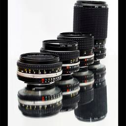
Flat hit@k (%)               Hierarchical precision@k
      Model type                dim        1        2      5       10        2       5        10      20
      Softmax baseline          N/A       55.6    67.4 78.5       85.0     0.452 0.342 0.313 0.319
      DeViSE                     500      53.2    65.2 76.7       83.3     0.447 0.352 0.331 0.341
                                1000      54.9    66.9 78.4       85.0     0.454 0.351 0.325 0.331
      Random embeddings          500      52.4    63.9 74.8       80.6     0.428 0.315 0.271 0.248
                                1000      50.5    62.2 74.2       81.5     0.418 0.318 0.290 0.292
      Chance                    N/A       0.1      0.2    0.5     1.0      0.007 0.013 0.022 0.042

Table 1: Comparison of model performance on our test set, taken from the ImageNet ILSVRC 2012 1K
validation set. Note that hierarchical precision@1 is equivalent to flat hit@1. See text for details.

ImageNet image repository [7]. In particular, for each true label and value of k, we generate a ground
truth list from the semantic hierarchy, and compute a per-example precision equal to the fraction of
the model’s k predictions that overlap with the ground truth list. We report mean precision across
the test set. Detailed descriptions of the generation of the ground truth lists, the hierarchical scoring
metric, and train/validation/test dataset splits are provided in Sections A.1 and A.3.

4.1   ImageNet (ILSVRC) 2012 1K Results

This section presents flat and hierarchical results on the ILSVRC 2012 1K dataset, where the classes
of the examples presented at test time are the same as those used for training. Table 1 shows results
for the DeViSE model for 500- and 1000-dimensional skip-gram models compared to the random
embedding and softmax baseline models, on both the flat and hierarchical metrics.6
On the flat metric, the softmax baseline shows higher accuracy for k = 1, 2. At k = 5, 10, the
1000-D DeViSE model has reached parity, and at k = 20 (not shown) it performs slightly better.
We expected the softmax model to be the best performing model on the flat metric, given that its
cross-entropy training objective is most well matched to the evaluation metric, and are surprised that
the performance of DeViSE is so close to softmax performance.
On the hierarchical metric, the DeViSE models show better semantic generalization than the soft-
max baseline, especially for larger k. At k = 5, the 500-D DeViSE model shows a 3% relative
improvement over the softmax baseline, and at k = 20 almost a 7% relative improvement. This is a
surprisingly large gain, considering that the softmax baseline is a reproduction of the best published
model on these data. The gap that exists between the DeViSE model and softmax baseline on the
hierarchical metric reflects the benefit of semantic information above and beyond visual similar-
ity [8]. The gap between the DeViSE model and the random embeddings model establishes that the
source of the gain is the well-structured embeddings learned by the language model not some other
property of our architecture.

4.2   Generalization and Zero-Shot Learning

A distinct advantage of our model is its ability to make reasonable inferences about candidate labels
it has never visually observed. For example, a DeViSE model trained on images labeled tiger shark,
bull shark, and blue shark, but never with images labeled shark, would likely have the ability to
generalize to this more coarse-grained descriptor because the language model has learned a repre-
sentation of the general concept of shark which is similar to all of the specific sharks. Similarly,
if tested on images of highly specific classes which the model has never seen before, for example
a photo of an oceanic whitecap shark, and asked whether the correct label is more likely oceanic
whitecap shark or some other unfamiliar label (say, nuclear submarine), our model stands a fight-
ing chance of guessing correctly because the language model ensures that representation of oceanic
whitecap shark is closer to the representation of sharks the model has seen, while the representation
of nuclear submarine is closer to those of other sea vessels.
   6
     Note that our softmax baseline results differ from the results in [11] due to a simplification in the evaluation
procedure: [11] creates several distorted versions of each test image and aggregates the results for a final label,
whereas in our experiments, we evaluate using only the original test image. Our softmax baseline is able to
reproduce the performance of the model in [11] when evaluated with the same procedure.

                                                         5
Our model              Softmax over ImageNet 1K                    Our model                   Softmax over ImageNet 1K
         A                                                                      D
             eyepiece, ocular            typewriter keyboard                         fruit                      pineapple, ananas
             Polaroid                    tape player                                 pineapple                  coral fungus
             compound lens               reflex camera                               pineapple plant, Ananas ...artichoke, globe artichoke
             telephoto lens, zoom lens   CD player                                   sweet orange               sea anemone, anemone
             rangefinder, range finder   space bar                                   sweet orange tree, ...     cardoon
         B                                                                      E
             oboe, hautboy, hautbois     reel                                        comestible, edible, ...      pot, flowerpot
             bassoon                     punching bag, punch bag, ...                dressing, salad dressing     cauliflower
             English horn, cor anglais   whistle                                     Sicilian pizza               guacamole
             hook and eye                bassoon                                     vegetable, veggie, veg       cucumber, cuke
             hand                        letter opener, paper knife, ...             fruit                        broccoli

         C                                                                      F
             barbet                      patas, hussar monkey, ...                   dune buggy, beach buggy      warplane, military plane
             patas, hussar monkey, ...   proboscis monkey, Nasalis ...               searcher beetle, ...         missile
             babbler, cackler            macaque                                     seeker, searcher, quester    projectile, missile
             titmouse, tit               titi, titi monkey                           Tragelaphus eurycerus, ...   sports car, sport car
             bowerbird, catbird          guenon, guenon monkey                       bongo, bongo drum            submarine, pigboat, sub, ...

Figure 2: For each image, the top 5 zero-shot predictions of DeViSE+1K from the 2011 21K label set and the
softmax baseline model, both trained on ILSVRC 2012 1K. Predictions ordered by decreasing score, with cor-
rect predictions in bold. Ground truth: (a) telephoto lens, zoom lens; (b) English horn, cor anglais; (c) babbler,
cackler; (d) pineapple, pineapple plant, Ananas comosus; (e) salad bar; (f) spacecraft, ballistic capsule, space
vehicle.

                                                                                            Flat hit@k (%)
                                                                 # Candidate
                   Data Set                Model                   Labels       1          2         5           10        20
                                           DeViSE-0                 1,589      6.0       10.0      18.1         26.4      36.4
                     2-hop
                                           DeViSE+1K                2,589      0.8        2.7       7.9         14.2      22.7
                                           DeViSE-0                 7,860      1.7        2.9       5.3         8.2       12.5
                     3-hop
                                           DeViSE+1K                8,860      0.5        1.4       3.4         5.9        9.7
                                           DeViSE-0                20,841      0.8        1.4       2.5         3.9        6.0
             ImageNet 2011 21K
                                           DeViSE+1K               21,841      0.3        0.8       1.9         3.2        5.3

Table 2: Flat hit@k performance of DeViSE on ImageNet-based zero-shot datasets of increasing difficulty
from top to bottom. DeViSE-0 and DeViSE+1K are the same trained model, but DeViSE-0 is restricted to only
predict zero-shot classes, whereas DeViSE+1K predicts both the zero-shot and the 1K training labels. For all,
zero-shot classes did not occur in the image training set.

To test this hypothesis, we extracted images from the ImageNet 2011 21K dataset with labels that
were not included in the ILSVRC 2012 1K dataset on which DeViSE was trained. These are “zero-
shot” data sets in the sense that our model has no visual knowledge of these labels, though embed-
dings for the labels were learned by the language model. The softmax baseline is only able to predict
labels from ILSVRC 2012 1K. The zero-shot experiments were performed with the same trained
500-D DeViSE model used for results in Section 4.1, but it is evaluated in two ways: DeViSE-0
only predicts the zero-shot labels, and DeViSE+1K predicts zero-shot labels and the ILSVRC 2012
1K training labels.
Figure 2 shows label predictions for a handful of selected examples from this dataset to qualitatively
illustrate model behavior. Note that DeViSE successfully predicts a wide range of labels outside
its training set, and furthermore, the incorrect predictions are generally semantically “close” to the
desired label. Figure 2 (a), (b), (c), and (d) show cases where our model makes significantly better
top-5 predictions than the softmax-based model. For example, in Figure 2 (a), the DeViSE model
is able to predict a number of lens-related labels even though it was not trained on images in any
of the predicted categories. Figure 2 (d) illustrates a case where the top softmax prediction is quite
good, but where it is unable to generalize to new labels and its remaining predictions are off the
mark, while our model’s predictions are more plausible. Figure 2 (e) highlights a case where neither
model gets the exact true label, but both models are giving plausible labels. Figure 2 (f) shows a
case where the softmax model emits more nearly correct labels than the DeViSE model.
To quantify the performance of the model on zero-shot data, we constructed from our ImageNet
2011 21K zero-shot data three test data sets of increasing difficulty based on the image labels’
tree distance from the training ILSVRC 2012 1K labels in the ImageNet label hierarchy [7]. The
easiest dataset, “2-hop”, is comprised of the 1,589 labels that are within two tree hops of the training
labels, making them visually and semantically similar to the training set. A more difficult “3-hop”
dataset was constructed in the same manner. Finally, we built a third, particularly challenging dataset
consisting of all the labels in ImageNet 2011 21K that are not in ILSVRC 2012 1K.

                                                                         6
Hierarchical precision@k
Data Set Model 1 2 5 10 20
DeViSE-0 0.06 0.152 0.192 0.217 0.233
2-hop DeViSE+1K 0.008 0.204 0.196 0.201 0.214
Softmax baseline 0 0.236 0.181 0.174 0.179
DeViSE-0 0.017 0.037 0.191 0.214 0.236
3-hop DeViSE+1K 0.005 0.053 0.192 0.201 0.214
Softmax baseline 0 0.053 0.157 0.143 0.130
DeViSE-0 0.008 0.017 0.072 0.085 0.096
ImageNet 2011 21K DeViSE+1K 0.003 0.025 0.083 0.092 0.101
Softmax baseline 0 0.023 0.071 0.069 0.065
Table 3: Hierarchical precision@k results on zero-shot classification. Performance of DeViSE compared to
the softmax baseline model across the same datasets as in Table 2. Note that the softmax model can never
directly predict the correct label so its precision@1 is 0.
Model 200 labels 1000 labels
DeViSE 31.8% 9.0%
Mensink et al. 2012 [12] 35.7% 1.9%
Rohrbach et al. 2011 [17] 34.8% -
Table 4: Flat hit@5 accuracy on the zero-shot task from [12]. DeViSE experiments were performed with a
500-D model. The [12] model uses a curated hierarchy over labels for zero-shot classification, but without using
this information, our model is close in performance on the 200 zero-shot class label task. When the models can
predict any of the 1000 labels, we achieve better accuracy, indicating DeViSE has less of a bias toward training
classes than [12]. As in [12], we include a result on a similar task from [17], though their work used a different
set of 200 zero-shot classes.
We again calculated the flat hit@k measure to determine how frequently DeViSE-0 and DeViSE+1K
predicted the correct label for each of these data sets (Table 2). DeViSE-0’s top prediction was the
correct label 6.0% of the time across 1,589 novel labels, and the rate increases with k to 36.4% within
the top 20 predictions. As the zero-shot data sets become more difficult, the accuracy decreases in
absolute terms, though it is better relative to chance (not shown). Since a traditional softmax visual
model can never produce the correct label on zero-shot data, its performance would be 0% for all
k. The DeViSE+1K model performed uniformly worse than the plain DeViSE-0 model by a margin
that indicates it has a bias toward training classes.
To provide a stronger baseline for comparison, we compared the performance of our model and
the softmax model on the hierarchical metric we employed above. Although the softmax baseline
model can never predict exactly the correct label, the hierarchical metric will give the model credit
for predicting labels that are in the neighborhood of the correct label in the ImageNet hierarchy
(for k > 1). Visual similarity is strongly correlated with semantic similarity for nearby object
categories [8], and the softmax model does leverage visual similarity between zero-shot and training
images to make predictions that will be scored favorably (e.g. Figure 2d).
The easiest dataset, “2-hop”, contains object categories that are as visually and semantically similar
to the training set as possible. For this dataset the softmax model outperforms the DeViSE model for
hierarchical precision@2, demonstrating just how large a role visual similarity plays in predicting
semantically “nearby” labels (Table 3). However, for k = 5, 10, 20, our model produces superior
predictions relative to the ImageNet hierarchy, even on this easiest dataset. For the two more diffi-
cult datasets, where there are more novel categories and the novel categories are less closely related
to those in the training data set, DeViSE outperforms the softmax model at all measured hierar-
chical precisions. The quantitative gains can be quite large, as much as 82% relative improvement
over softmax performance, and qualitatively, the softmax model’s predictions can be surprisingly
unreasonable in some cases (e.g. Figure 2c). The random embeddings model we described above
performed substantially worse than either of the real models. These results indicate that our archi-
tecture succeeds in leveraging the semantic knowledge captured by the language model to make
reasonable predictions, even as test images become increasingly dissimilar from those used in the
training set.
To provide a comparison with other work in zero-shot learning, we also directly compare to the
zero-shot results from [12]. These were performed on a particular 800/200 split of the 1000 classes
7from ImageNet 2010: training and model tuning is performed using the 800 classes, and test images
are drawn from the remaining 200 classes. Results are shown in Table 4.
Taken together, these zero-shot experiments indicate that the DeViSE model can exploit both visual
and semantic information to predict novel classes never before observed. Furthermore, the presence
of semantic information in the model substantially improves the quality of its predictions.
5 Conclusion
In contrast to previous attempts in this area [18], we have shown that our joint visual-semantic em-
bedding model can be trained to give performance comparable to a state-of-the-art softmax based
model on a flat object classification metric, while simultaneously making more semantically rea-
sonable errors, as indicated by its improved performance on a hierarchical label metric. We have
also shown that this model is able to make correct predictions across thousands of previously unseen
classes by leveraging semantic knowledge elicited only from unannotated text.
The advantages of this architecture, however, extend beyond the experiments presented here.
First, we believe that our model’s unusual compatibility with larger, less manicured data sets will
prove to be a major strength moving forward. In particular, the skip-gram language model we
constructed included only a modestly sized vocabulary, and was exposed only to the text of a single
online encyclopedia; we believe that the gains available to models with larger vocabularies and
trained on vastly larger text corpora will be significant, and easily outstrip methods which rely on
manually constructed semantic hierarchies (e.g. [17]). Perhaps more importantly, though here we
trained on a curated academic image dataset, our model’s architecture naturally lends itself to being
trained on all available images that can be annotated with any text term contained in the (larger)
vocabulary. We believe that training massive “open” image datasets of this form will dramatically
improve the quality of visual object categorization systems.
Second, we believe that the 1-of-N (and nearly balanced) visual object classification problem is
soon to be outmoded by practical visual object categorization systems that can handle very large
numbers of labels [5] and the re-definition of valid label sets at test time. For example, our model
can be trained once on all available data, and simultaneously used in one application requiring
only coarse object categorization (e.g. house, car, pedestrian) and another application requiring
fine categorization in a very specialized subset (e.g. Honda Civic, Ferrari F355, Tesla Model-S).
Moreover, because test time computation can be sub-linear in the number of labels contained in the
training set, our model can be used in exactly such systems with much larger numbers of labels,
including overlapping or never-observed categories.
Moving forward, we are experimenting with techniques which more directly leverage the structure
inherent in the learned language embedding, greatly reducing training costs of the joint model and
allowing even greater scaling [15].
Acknowledgments
Special thanks to those who lent their insight and technical support for this work, including Matthieu
Devin, Alex Krizhevsky, Quoc Le, Rajat Monga, Ilya Sutskever, and Wojciech Zaremba.
References
[1] S. Bengio, J. Weston, and D. Grangier. Label embedding trees for large multi-class tasks. In Advances in
Neural Information Processing Systems, NIPS, 2010.
[2] Y. Bengio, R. Ducharme, and P. Vincent. A neural probabilistic language model. Journal of Machine
Learning Research, 3:1137–1155, 2003.
[3] A. Coates and A. Ng. The importance of encoding versus training with sparse coding and vector quanti-
zation. In International Conference on Machine Learning (ICML), 2011.
[4] Jeffrey Dean, Greg S. Corrado, Rajat Monga, Kai Chen, Matthieu Devin, Quoc V. Le, Mark Z. Mao,
MarcAurelio Ranzato, Andrew Senior, Paul Tucker, Ke Yang, and Andrew Y. Ng. Large scale distributed
deep networks. In Advances in Neural Information Processing Systems, NIPS, 2012.
8[5] Thomas Dean, Mark Ruzon, Mark Segal, Jonathon Shlens, Sudheendra Vijayanarasimhan, and Jay Yag-
nik. Fast, accurate detection of 100,000 object classes on a single machine. In IEEE Conference on
Computer Vision and Pattern Recognition (CVPR), 2013.
[6] Jia Deng, Alex Berg, Sanjeev Satheesh, Hao Su, Aditya Khosla, and Fei-Fei Li. Imagenet large scale
visual recognition challenge 2012.
[7] Jia Deng, Wei Dong, Richard Socher, Li jia Li, Kai Li, and Li Fei-fei. Imagenet: A large-scale hierarchical
image database. In IEEE Conference on Computer Vision and Pattern Recognition (CVPR), 2009.
[8] Thomas Deselaers and Vittorio Ferrari. Visual and semantic similarity in imagenet. In IEEE Conference
on Computer Vision and Pattern Recognition (CVPR), 2011.
[9] J. C. Duchi, E. Hazan, and Y. Singer. Adaptive subgradient methods for online learning and stochastic
optimization. Journal of Machine Learning Research, 12:2121–2159, 2011.
[10] Geoffrey E. Hinton, Nitish Srivastava, Alex Krizhevsky, Ilya Sutskever, and Ruslan R. Salakhutdi-
nov. Improving neural networks by preventing co-adaptation of feature detectors. arXiv preprint
arXiv:1207.0580, 2012.
[11] Alex Krizhevsky, Ilya Sutskever, and Geoffrey E. Hinton. Imagenet classification with deep convolutional
neural networks. In Advances in Neural Information Processing Systems, NIPS, 2012.
[12] Thomas Mensink, Jakob Verbeek, Florent Perronnin, and Gabriela Csurka. Metric learning for large scale
image classification: Generalizing to new classes at near-zero cost. In European Conference on Computer
Vision (ECCV), 2012.
[13] Tomas Mikolov, Kai Chen, Greg S. Corrado, and Jeffrey Dean. Efficient estimation of word represen-
tations in vector space. In International Conference on Learning Representations (ICLR), Scottsdale,
Arizona, USA, 2013.
[14] Tomas Mikolov, Ilya Sutskever, Kai Chen, Greg Corrado, and Jeffrey Dean. Distributed representations
of words and phrases and their compositionality. In Advances in Neural Information Processing Systems,
NIPS, 2013.
[15] Mohammad Norouzi, Tomas Mikolov, Samy Bengio, Jonathon Shlens, Andrea Frome, Greg S. Corrado,
and Jeffrey Dean. Zero-shot learning by convex combination of semantic embeddings. arXiv (to be
submitted), 2013.
[16] Mark Palatucci, Dean Pomerleau, Geoffrey E. Hinton, and Tom M. Mitchell. Zero-shot learning with
semantic output codes. In Advances in Neural Information Processing Systems, NIPS, 2009.
[17] Marcus Rohrbach, Michael Stark, and Bernt Schiele. Evaluating knowledge transfer and zero-shot learn-
ing in a large-scale setting. In IEEE Conference on Computer Vision and Pattern Recognition (CVPR),
2011.
[18] R. Socher, M. Ganjoo, H. Sridhar, O. Bastani, C. D. Manning, and A. Y. Ng. Zero-shot learning through
cross-modal transfer. In International Conference on Learning Representations (ICLR), Scottsdale, Ari-
zona, USA, 2013.
[19] L.J.P. van der Maaten and G.E. Hinton. Visualizing high-dimensional data using t-sne. Journal of Machine
Learning Research, 9:2579–2605, 2008.
[20] Jason Weston, Samy Bengio, and Nicolas Usunier. Large scale image annotation: learning to rank with
joint word-image embeddings. Machine Learning, 81(1):21–35, 2010.
A Appendix
A.1 Validation/test Data Methodology
For all experiments except the comparison to Mensink et al. [12] we train our visual model and
DeViSE on the ILSVRC 2012 1K data set. Experiments in Section 4.1 use images and labels only
from the 2012 1K set for testing, and the zero-shot experiments in Section 4.2 use image and labels
from the ImageNet 2011 21K set and, for DeViSE+1K, also labels from ILSVRC 2012 1K. The
same subset of the ILSVRC 2012 1K data used to train the visual model (Section 3.2) is also used to
train DeViSE and the random embedding-based models, and when training all models, we randomly
flip, crop and translate images to artificially expand the training set several-fold. The 50K images
from the ILSVRC 2012 1K validation set are split randomly 10/90 into our experimental validation
and held-out test sets of 5K and 45K images, respectively. Our validation set is used to choose
hyperparameters, and results are reported on the held-out set. The 1,000 classes are roughly balanced
in the validation and held-out sets. The 500-D DeViSE model trained for the experiments in Section
4.1 is also used for the corresponding zero-shot experiments in Section 4.2 with no additional tuning.
9The zero-shot experiments performed to compare to Mensink et al. [12] are trained with images
and labels from the ILSVRC 2010 1K data set, using the same 800/200 training/test class split used
in [12]. We use the ILSVRC 2010 training/validation/test data split; training and validation images
from the 800 classes are used to train and tune our visual model and DeViSE, and test images from
the 200 zero-shot classes are used to generate our experimental results.
At test time, images are center-cropped to 225 × 225 for input to the visual model, and no other
distortions are applied.
A.2 Mapping Text Terms to ImageNet Synset
The language model represents terms and phrases gathered from unannotated text as embedding
vectors, whereas the ImageNet data set represents each class as a synset, a set of synonymous terms,
where each term is a word or phrase. When training DeViSE, a method is needed for mapping from
an ImageNet synset to the target embedding vector, and at prediction time, label predictions from the
embedding space must be translated back into ImageNet synsets from the test set for scoring. There
are two complications: (1) the same term can occur in multiple ImageNet synsets, often representing
different concepts, for example the two synsets consisting only of “crane” in ILSVRC 2012 1K; (2)
the language model as we have trained it only has one embedding for each word or phrase, so there
is only one embedding vector representing both senses of “crane”.
When training, we choose the target embedding vector by mapping the first term of the synset to its
embedding vector through the text of the synset term. We found this to work well in practice; other
possible approaches are to choose randomly from among the synset terms or take an average of the
embedding vectors for the synset terms.
When making a prediction, the mapping from embedded text vectors back to ImageNet synsets
is more difficult: each embedding vector can correspond to several ImageNet synsets due to the
repetition of terms between synsets, up to 9 different synsets in the case of “head”. Additionally,
multiple of our predicted embedding vectors can correspond to terms from the same synset, e.g.
“ballroom”, “dance hall”, “dance palace”. In practice, this happens frequently since synonymous
terms are embedded close to one another by the skip-gram language model.
For a given visual output vector, our model first finds the N nearest embedding label vectors using
cosine similarity, sorted by their similarity, where N > k. In these experiments, we chose N = 4 ∗ k
as this is close to the average number of text labels per synset in the ILSVRC 2012 data set. The
first step in converting these to ImageNet synsets is to expand every embedded term to all of its
corresponding ImageNet synsets. For example, “crane” would be expanded to the two synsets which
contain the term “crane” (the order of the two “crane” synsets in the final list is arbitrary). After
expansion, if there are duplicate entries for a given synset, then all but the first are removed from
their places in the list, leaving a list where each synset occurs at most once in the prediction list.
Finally, the list is truncated to the top k predictions. We experimented with choosing randomly from
among all the possible synsets instead of expanding to all of them and found this to slightly reduce
performance in the ILSVRC 2012 1K experiments.
A.3 Hierarchical Precision-at-k Metric
We defined the following hierarchical precision-at-k metric, hp@k, to assess the accuracy of model
predictions with respect to the ImageNet object category hierarchy. For each image in the test set, the
model in question emits its top k predicted ImageNet object category labels (synsets). We calculate
hp@k as the fraction of these k predictions which are in hCorrectSet, averaged across the test
examples:
N
1 X number of model’s top k predictions in hCorrectSet for image i
hp@k = (2)
N i=1 k
The hCorrectSet for a true label is constructed by iteratively adding nodes from the ImageNet
hierarchy in a widening radius around the true label until hCorrectSet has a size ≥ k:
hCorrectSet = {}
R = 0
10k
Label set # kCorrectSet Labels 2 5 10 20
ImageNet 2012 1K 1000 6.5 12.5 22.5 41.7
Zero-shot 2-hop 2589 3.2 16.8 25.5 45.2
Zero-shot 3-hop 8860 4.4 577.4 635.4 668.0
Zero-shot ImageNet 2011 21K 21900 5.4 273.3 317.4 350.6
Table 5: Mean sizes of hCorrectSet lists used for hierarchical evaluation, averaged across the test examples,
shown for various label sets and values of k. At k = 1, hCorrectSet always contains only the true label.
Note that for the zero-shot data sets, kCorrectSet includes the test set labels as well as the ImageNet 2012
1K labels. List sizes vary among test examples depending upon the local topology of the graph around the true
label as well as how many labels from the graph are in the ground truth set.
while NumberElements(hCorrectSet < k):
radiusSet = all nodes in the ImageNet hierarchy which are
R hops from the true label
validRadiusSet = ValidLabelNodes(radiusSet)
hCorrectSet = Union(hCorrectSet, validRadiusSet)
R = R + 1
return hCorrectSet
The size of hCorrectSet for a given test example depends on the combination of the structure of
the hierarchy around a given label and which classes are included in the test set. It is exactly 1 when
k = 1 and is rarely equal to k when k > 1. The ValidLabelNodes()function allows us to
restrict hCorrectSet to any subset of labels in the ImageNet (or larger WordNet) hierarchy. For
example, in generating the results in Table 2 we restrict the nodes in the hCorrectSet to be drawn
from only those nodes which are both members the ImageNet 2011 21K label set and are three-hops
or less from at least one of the ImageNet 2012 1K labels.
Note that this hierarchical metric differs from the hierarchical metric used in some of the earlier
ImageNet Challenge competitions. That metric was generally considered to be rather insensitive,
and was withdrawn from more recent years of the competition. Our DeViSE model does perform
better than the baseline softmax model on that metric as well, but effect sizes are generally much
smaller.
11You can also read