A Unified Survey on Anomaly, Novelty, Open-Set, and Out- of-Distribution Detection: Solutions and Future Challenges
←
→
Page content transcription
If your browser does not render page correctly, please read the page content below
Under review as submission to TMLR

                                        A Unified Survey on Anomaly, Novelty, Open-Set, and Out-
                                        of-Distribution Detection: Solutions and Future Challenges

                                        Mohammadreza Salehi
                                        University of Amsterdam
                                        Hossein Mirzaei
                                        Sharif University of Technology
                                        Dan Hendrycks
                                        UC Berkeley
                                        Yixuan Li
arXiv:2110.14051v4 [cs.CV] 7 Jul 2022

                                        University of Wisconsin-Madison
                                        Mohammad Hossein Rohban
                                        Sharif University of Technology
                                        Mohammad Sabokrou
                                        Institute For Research In Fundamental Sciences(IPM)

                                                                                          Abstract

                                                Machine learning models often encounter samples that are diverged from the training distri-
                                                bution. Failure to recognize an out-of-distribution (OOD) sample, and consequently assign
                                                that sample to an in-class label, significantly compromises the reliability of a model. The
                                                problem has gained significant attention due to its importance for safety deploying mod-
                                                els in open-world settings. Detecting OOD samples is challenging due to the intractability
                                                of modeling all possible unknown distributions. To date, several research domains tackle
                                                the problem of detecting unfamiliar samples, including anomaly detection, novelty detec-
                                                tion, one-class learning, open set recognition, and out-of-distribution detection. Despite
                                                having similar and shared concepts, out-of-distribution, open-set, and anomaly detection
                                                have been investigated independently. Accordingly, these research avenues have not cross-
                                                pollinated, creating research barriers. While some surveys intend to provide an overview
                                                of these approaches, they seem to only focus on a specific domain without examining the
                                                relationship between different domains. This survey aims to provide a cross-domain and
                                                comprehensive review of numerous eminent works in respective areas while identifying their
                                                commonalities. Researchers can benefit from the overview of research advances in differ-
                                                ent fields and develop future methodology synergistically. Furthermore, to the best of our
                                                knowledge, while there are surveys in anomaly detection or one-class learning, there is
                                                no comprehensive or up-to-date survey on out-of-distribution detection, which this sur-
                                                vey covers extensively. Finally, having a unified cross-domain perspective, this study dis-
                                                cusses and sheds light on future lines of research, intending to bring these fields closer
                                                together. All the implementations and benchmarks reported in the paper can be found at :
                                                https://github.com/taslimisina/osr-ood-ad-methods

                                        1   Introduction

                                        Machine learning models commonly make the closed-set assumption, where the test data is drawn i.i.d from
                                        the same distribution as the training data. Yet in practice, all types of test input data—even those on
                                        which the classifier has not been trained—can be encountered. Unfortunately, models can assign misleading
                                        confidence values for unseen test samples Sun et al. (2020); Miller et al. (2021); Oza & Patel (2019); Yoshihashi
                                        et al. (2019); Yu & Aizawa (2019). This leads to concerns about the reliability of classifiers, particularly for
                                        safety-critical applications Hendrycks et al. (2021a). In the literature, several fields attempt to address the
                                        issue of identifying the unknowns/anomalies/out-of-distribution data in the open-world setting. In particular,

                                                                                               1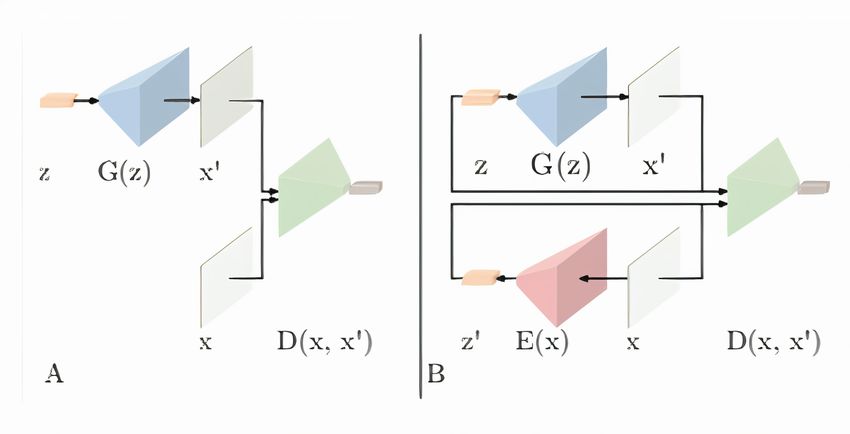
Under review as submission to TMLR

the problems of anomaly detection (AD), Novelty Detection (ND), One-Class Classification (OCC), Out-of-
Distribution (OOD) detection, and Open-Set Recognition (OSR) have gained significant attention owing to
their fundamental importance and practical relevance. They have been used for similar tasks, although the
differences and connections are often overlooked.
Specifically, OSR trains a model on K classes of a N class training dataset; then, at the test time, the
model is faced with N different classes of which N − K are not seen during training. OSR aims to assign
correct labels to seen test-time samples while detecting the unseen samples. Novelty detection or one-class
classification is an extreme case of open-set recognition, in which K is 1. In the multi-class classification
setting, the problem of OOD detection is canonical to OSR: accurately classify in-distribution (ID) samples
into the known categories and detect OOD data that is semantically different and therefore should not
be predicted by the model. However, OOD detection encompasses a broader spectrum of learning tasks
(e.g., multi-label classification, reinforcement learning) and solution space (e.g., density estimation), which
is comprehensively reviewed in this paper.
While all the aforementioned domains hold the assumption of accessing an entirely normal training dataset,
anomaly detection assumes the training dataset is captured in a fully unsupervised manner without applying
any filtration; therefore, it might contain some abnormal samples too. However, as abnormal events barely
occur, AD methods have used this fact and proposed filtering during the training process to reach a final
semantic space that fully grasps normal features. Despite previous approaches that are mostly used in object
detection and image classification domains, this setting is more common in the industrial defect detection
tasks, in which abnormal events are rare and normal samples have a shared concept of normality. Fig. 1
depicts an overview of the mentioned domains, in which the differences are shown visually. Note that even
if there are differences in the formulation of these domains, they have so much in common, and are used
interchangeably.
As an important research area, there have been several surveys in the literature Bulusu et al. (2020); Perera
et al. (2021); Ruff et al. (2021); Pang et al. (2020); Chalapathy & Chawla (2019), focusing on each domain
independently or providing a very general notion of anomaly detection to cover all different types of datasets.
Instead, this paper in-depth explanations for methodologies in respective areas. We make cross-domain
bridges by which ideas can be easily propagated and inspire future research. For instance, the idea of using
some outlier samples from different datasets to improve task-specific features is called Outlier Exposure in
Hendrycks et al. (2019a) or background modeling in Dhamija et al. (2018), and is very similar to semi-
supervised anomaly detection in Ruff et al. (2019). Despite the shared idea, all are considered to be novel
ideas in their respective domains.
In this survey, we identify the commonalities that address different but related fields. Furthermore, we
try to categorize different methods based on general justifications. For instance, some surveys Ruff et al.
(2021); Yang et al. (2021) categorize methods into different classes, such as distance-based methods and
density-based methods. As distance-based methods can be simply converted to density-based ones, one can
find this classification ambiguous. Although some of the mentioned tasks have very close methodological
setups, they differ in their testing protocols. Therefore, a comprehensive review of all the methods can better
reveal their limitations in practical applications. As a Key part to this survey, methods are described both
mathematically and visually to give better insights to both newcomers and experienced researchers. Finally,
comprehensive future lines of research are provided both practically and fundamentally to not only address
the issues of current methods but also shed light on critical applications of these methods in different fields.
In summary, the main contributions are as follows :

     1. Identification of the relationship between different research areas that, despite being highly correlated
        with each other, have been examined separately.

     2. Comprehensive methodological analysis of recent eminent research, and providing a clear theoretical
        and visual explanation for methods reviewed.

     3. Performing comprehensive tests on existing baselines in order to provide a solid ground for current
        and future lines of research.

                                                       2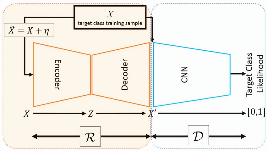
Under review as submission to TMLR

     4. Providing plausible future lines of research and specifying some fundamental necessities of the meth-
        ods that will be presented in the future such as fairness, adversarial robustness, privacy, data-
        efficiency, and explainability.

      Novelty Detection

      Open-Set Recognition

      Out-Of-Distribution Detection                                                              ND       One-class
                                                                                                        classification
                                                                                                             loss
                                                                       [ A ]vs[ B ∪ C ]

                                                                                                         Multi-class
                                                                                                 OSR    classification
                                                                       [ A ∪ B ]vs[ C ]                      loss

                                          A

                                                 B
                                                                                                         Multi-class
                                                                                                 OOD
                                                                                                        classification
                                                        C              [ A ∪ B ]vs[ C ∪ D ]                  loss

                                                              D

Figure 1: Problem setup for ND, OSR, and ODD from a unified perspective based on the common routine
followed in the respective fields. (A), (B) and (C) are sampled from the same training dataset, while
(D) is sampled from different datasets. Typically, in ND, all training samples are deemed normal, and
share a common semantic (green region), while samples diverged from such distribution are considered as
anomalous. Although samples in area (D) can be regarded as potential outliers, only areas (B) and (C) are
used as anomalies for the evaluation phase. In OSR, more supervision is available by accessing the label of
normal samples. For example "car", "dog", "cat", and "airplane" classes i.e, the union of (A) and (B), are
considered as normal while (C) is open-set distribution(see right Figure). Same as ND, (D) is not usually
considered an open-set distribution in the field, while there is no specific constraint on the type of open-set
distribution in the definition of OSR domain. In OOD detection, multiple classes are considered as normal,
which is quite similar to OSR. For example, (A), (B), and (C) comprise the normal training distributions,
and another distribution that shows a degree of change with respect to the training distribution and is said
to be out-of-distribution, which can be (D) in this case.

2   A Unified Categorization

Consider a dataset with training samples (x1 , y1 ), (x2 , y2 ), ... from the joint distribution PX,Y , where X and
Y are random variables on an input space X = Rd and a label (output) space Y respectively. In-class (also
called "seen" or "normal") domain refers to the training data. In AD or ND, the label space Y is a binary
set, indicating normal vs. abnormal. During testing, provided with an input sample x, the model needs to
estimate P (Y = normal/seen/in-class | X = x) in the cases of one-class setting. In OOD detection and OSR
for multi-class classification, the label space can contain multiple semantic categories, and the model needs
to additionally perform classification on normal samples based on the posterior probability p(Y = y | x).
It is worth mentioning that in AD, input samples could contain some noises (anomalies) combined with
normals; thus, the problem is converted into a noisy-label one-class classification problem; however, the
overall formulation of the detection task still remains the same.

                                                        3
Under review as submission to TMLR

      Novelty Detection Methods

      Open-Set Recognition Methods                   Unfamiliar Data Detection Approaches                                                            Anomaly Detection
      Out-Of-Distribution Detection Methods

  Pre-trained Feature                                                                                    Generative
                                          Discriminative

                                                                                                                                                                            Increasing Supervision
      Adaptation

                                                                                                                                                     Novelty Detection
                   Self Supervised Learning                Classification Based           Autoencoders        Generative Adversarial Networks

                                                      One-Class           Multi-Class
                                                     Classification      Classification

     [6, 8]      [5, 7]        [13]           [20]        [3]         [15, 13] [16-24]    [1, 2]       [11]      [1]       [14] [10, 14] Out-of-Distribution   Open Set Recognition
                                                                                                                                                Detection

Figure 2: As discussed in section 2, all unfamiliar sample detection approaches can be unitedly classified
in the shown hierarchical structure. The tree on the right points out that although some approaches have
been labeled as ND, OSR, or OOD detection in the field, however can be classified in a more grounded and
general form such that their knowledge could be shared synergistically. For instance, self-supervised ND
methods can be added to multi-class classification approaches without harming their classification assump-
tions. Unfamiliar sample detection can be done by employing different levels of supervision, which is shown
on the left.

To model the conditional probabilities, the two most common and known perspectives are called generative
modeling and discriminative modeling. While discriminative modeling might be easy for OOD detection
or OSR settings since there is access to the labels of training samples; nevertheless, the lack of labels makes
AD, ND (OCC) challenging. This is because one-class classification problems have a trivial solution to map
each of their inputs regardless of being normal or anomaly to the given label Y and, consequently, minimize
their objective function as much as possible. This issue can be seen in some of the recent approaches such as
DSVDDRuff et al. (2018), which maps every input to a single point regardless of being normal or abnormal
when it is trained for a large number of training epochs.
Some approaches Golan & El-Yaniv (2018); Bergman & Hoshen (2020), however, have made some changes
in the formulation of P (Y | X) to solve this problem. They apply a set of affine transformations on the
                                                                                                  P|T |
distribution of X such that the normalized distribution does not change. Then the summation i=1 P (Ti |
Ti (X)) is estimated, calculating the aggregated probability of each transformation Ti being applied on the
input X given the transformed input Ti (X), which is equal to |T |P (Y | X). This is similar to estimating
P (Y | X) directly; however, it would not collapse and can be used instead of estimating one-class conditional
probability. This simple approach circumvents the problem of collapsing; however, it makes the problem
dependent on the transformations since transformed inputs must not intersect with each other as much as
possible to satisfy the constraint of normalized distribution consistency. Therefore, as elaborated later in
the survey, OSR methods can employ AD approaches with classification models to overcome their issues. A
similar situation holds for the OOD domain.
In generative modeling, AE (Autoencoder)-based, GAN (Generative Adversarial Network)-based, and ex-
plicit density estimation-based methods such as auto-regressive and flow-based models are used to model
the data distribution. For AEs, there are two important assumptions.
If the auto-encoder is trained solely on normal training samples:

        • They would be able to reconstruct unseen normal test-time samples as precisely as training time
          ones.

        • They would not be able to reconstruct unseen abnormal test-time samples as precisely as normal
          inputs.

                                                                                                   4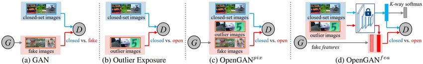
Under review as submission to TMLR

Table 1: The table summarizes the most notable recent deep learning-based works in different fields, specified
by the informative methodological keywords and decision score used in each work. For the methods that have
common parts, a shared set of keywords are used to place them on a unitary ground as much as possible.
The pros and cons of each methodology are described in detail in the method explanation.

Taxonomy   Index        Methods                   Refrence                              Decision Score                                                                                         Keywords

             1           ALOCC                Sabokrou et al. (2018a)                reconstruction error for input                   discriminative-generative, reconstruction-based, adversarial learning, denoising AutoEncoder, Refinement and Detection

             2           Mem-AE                 Gong et al. (2019)                   reconstruction error for input                    generative, reconstruction-based, Memory-based Representation, sparse addressing technique, hard shrinkage operator

             3          DeepSvdd                 Ruff et al. (2018)                   distance of the input to the                              discriminative, extension of SVDD, compressed features, minimum volume hyper-sphere, Autoencoder
                                                                                       center of the hypersphere

             4              GT               Golan & El-Yaniv (2018)          sum of Dirichlet probabilities for different                self-supervised learning, auxiliary task, self-labeled dataset, geometric transformations, softmax response vector
                                                                                        transformations of input
  ND
             5              CSI                  Tack et al. (2020)        cosine similarity to the nearest training sample                   self-supervised learning, contrastive learning, negative samples, shifted distribution, hard augmentations
                                                                               multiplied by the norm of representation

             6     Uninformed Students        Bergmann et al. (2020)               an ensemble of student networks’                       knowledge distillation, teacher-student based, transfer learning, self supervised learning, Descriptor Compactness
                                                                                     variance and regression error

             7           CutPaste                 Li et al. (2021)        log-density of trained Gaussian density estimator             self-supervised Learning, generative classifiers, auxiliary task, extracting patch-level representations, cutout and scar

             8          Multi-KD               Salehi et al. (2021b)      discrepancy between the intermediate teacher and          knowledge distillation, teacher-student, transfer the intermediate knowledge, pretrained network, mimicking different layers
                                                                                  student networks’ activation values

             9           OpenMax             Bendale & Boult (2016)      after computing OpenMax probability per channel                      Extreme Value Theorem, activation vector, overconfident scores, weibull distribution, Meta-Recognition
                                                                                maximum probability is then selected

            10            OSRCI                  Neal et al. (2018)      probability assigned to class with label k + 1, minus             generative, unknown class generation, classification based, Counterfactual Images, learning decision boundary
                                                                            maximum probability assigned to first k class
                                                                                                                                     generative, Reconstruction based, class conditional Autoencoder, Extreme Value Theory, feature-wise linear modulations
  OSR       11             C2AE                 Oza & Patel (2019)        minimum reconstruction error under different match
                                                                          vectors, compared with the predetermined threshold
                                                                                                                                      discriminative-generative, classification-reconstruction based , Extreme Value Theorem, hierarchical reconstruction nets
            12           CROSR                Yoshihashi et al. (2019)   after computing OpenMax probability per channel
                                                                                maximum probability is then selected

            13            GDFR                  Perera et al. (2020)      by passing the augmented input to the classifier               discriminative-generative, self-supervised learning, reconstruction based, auxiliary task, geometric transformation
                                                                             network, and finding maximum activation

            14           OpenGan             Kong & Ramanan (2021)               the trained discriminator utilized as             discriminative-generative, unknown class generation, adversarially synthesized fake data, crucial to use a validation set, model selection
                                                                                    an open-set likelihood function

            15             MLS                   Vaze et al. (2021)               negation of maximum logit score                     discriminative, classification based, between the closed-set and open-set, Fine-grained datasets, Semantic Shift Benchmark(SSB)

            16             MSP              Hendrycks & Gimpel (2016)        Negation of maximum softmax probability                    outlier detection metric, softmax distribution, maximum class probability, classification based, various data domains

            17             ODIN                 Liang et al. (2017)          Negation of maximum softmax probability                  outlier detection metric, softmax distribution, temperature scaling, adding small perturbations, enhancing separability
                                                                                     with temperature scaling

            18      A Simple Unified etc.        Lee et al. (2018)               Mahalanobis distance to the closest                    distance based, simple outlier detection metric, small controlled noise, class-incremental learning, Feature ensemble
                                                                                    class-conditional Gaussian

            19              OE                Hendrycks et al. (2018)         negation of maximum softmax probability                    outlier exposure , auxiliary dataset, classification based, uniform distribution over k classes, various data domains

  OOD       20        Using SSL etc.         Hendrycks et al. (2019a)        negation of maximum softmax probability                       self-supervised learning, auxilary task, robustness to adversarial perturbations, MSP, geometric transformation

            21           G-ODIN                  Hsu et al. (2020)             softmax output’s categorical distribution                        outlier detection metric, softmax distribution, learning temperature scaling, Decomposed Confidence

            22     Energy-based OOD              Liu et al. (2020b)                       the energy function                      outlier detection metric, hyperparameter-free, The Helmholtz f ree energy, energy-bounded learning, the Gibbs distribution
                                                                             (a scalar is derived from the logit outputs)

            23             MOS                  Wang et al. (2021)              lowest others score among all groups                           softmax distribution, group-based Learning, large-scale images, category others, pre-trained backbone

            24            ReAct                  Sun et al. (2021)       after applying ReAct different OOD detection methods                  activation truncation, reducing model overconfidence, compatible with different OOD scoring functions
                                                                          could be used. they default to using the energy score.

Nevertheless, recently proposed AE-based methods show that the above-mentioned assumptions are not
always true Salehi et al. (2021a); Gong et al. (2019); Zaheer et al. (2020). For instance, even if AE can
reconstruct normal samples perfectly, nonetheless with only a one-pixel shift, reconstruction loss will be
high.
Likewise, GANs as another famous model family, are widely used for AD, ND, OCC, OSR, and OOD
detection. If a GAN is trained on fully normal training samples, it operates on the following assumptions:

       • If the input is normal then there is a latent vector that, if generated, has a low discrepancy with
         the input.

       • If the input is abnormal then there is not a latent vector that, if generated, has a low discrepancy
         with the input.

Here, the discrepancy can be defined based on the pixel-level MSE loss of the generated image and test
time input or more complex functions such as layer-wise distance between the discriminator’s features when
fed a generated image and test-time input. Although GANs have proved their ability to capture semantic

                                                                                                                      5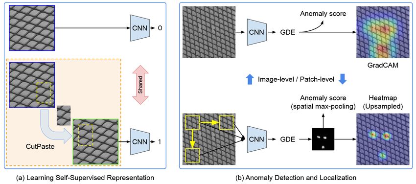
Under review as submission to TMLR

abstractions of a given training dataset, they suffer from mode-collapse, unstable training process, and
irreproducible result problems Arjovsky & Bottou (2017).
Finally, auto-regressive and flow-based models can be used to explicitly approximate the data density and
detect abnormal samples based on their assigned likelihood. Intuitively, normal samples must have higher
likelihoods compared to abnormal ones; however, as will be discussed later, auto-regressive models assign
even higher amount of likelihoods to abnormal samples despite them not being seen in the training phase,
which results in a weak performance in AD, ND, OSR, and OOD detection.Solutions to this problem will
be reviewed in subsequent sections. To address this issue, several remedies have been proposed in the
OOD detection domain, which can be used in OSR, AD, and ND; however, considering the fact that OOD
detection’s prevalent testing protocols might be quite different from other domains such as AD or ND,
more evaluations on their reliability are needed. As lots of works with similar ideas or intentions have
been proposed in each domain, we mainly focus on providing a detailed yet concise summary of each and
highlighting the similarities in the explanations. In Table 1 and Fig. 2, a summary of the most notable
papers reviewed in this work is presented along with specifications on their contributions with respect to the
methodological categorization provided in this paper.

3     Non-Deep Learning-Based Approaches

In this section, some of the most notable traditional methods used to tackle the problem of anomaly detection
are explained. All other sections are based on the new architectures that are mainly based on deep learning.

3.1   Isolation Forests Liu et al. (2008):

Like Random Forests, Isolation Forests (IF) are constructed using decision trees. It is also an unsupervised
model because there are no predefined labels. Isolation Forests were created with the notion that anomalies
are "few and distinct" data points. An Isolation Forest analyzes randomly sub-sampled data in a tree
structure using attributes chosen at random. As further-reaching samples required more cuts to separate,
they are less likely to be outliers. Similarly, samples that end up in shorter branches exhibit anomalies
because the tree could distinguish them from other data more easily. Fig. 3 depicts the overall procedure of
this work.

Figure 3: An overview of the isolation forest method is shown. Anomalies are more susceptible to isolation
and hence have short path lengths. A normal point xi requires twelve random partitions to be isolated
compared to an anomaly xo that requires only four partitions to be isolated.

                                                      6
Under review as submission to TMLR

3.2   DBSCAN Ester et al. (1996):

Given a set of points in a space, DBSCAN combines together points that are densely packed together (points
with numerous nearby neighbors), identifying as outliers those that are isolated in low-density regions. The
steps of the DBSCAN algorithm are as follows: (1) Identify the core points with more than the minimum
number of neighbors required to produce a dense zone. (2) Find related components of core points on the
neighbor graph, ignoring all non-core points.(3) If the cluster is a neighbor, assign each non-core point to it,
otherwise assign it to noise. Fig. 4 depicts the overall procedure of this work.

Figure 4: The minimal number of points required to generate a dense zone in this figure is four. Since the
area surrounding these points in a radius contains at least four points, Point A and the other red points are
core points (including the point itself). They constitute a single cluster because they are all reachable from
one another. B and C are not core points, but they may be reached from A (through other core points) and
hence are included in the cluster. Point N is a noise point that is neither a core nor reachable directly.

3.3   LOF: Identifying Density-Based Local Outliers Breunig et al. (2000):

The local outlier factor is based on the concept of a local density, in which locality is determined by the
distance between K nearest neighbors. One can detect regions of similar density and points that have a
significantly lower density than their neighbors by comparing the local density of an object to the local
densities of its neighbors. These are classified as outliers. The typical distance at which a point can
be "reached" from its neighbors is used to estimate the local density. The LOF notion of "reachability
distance" is an extra criterion for producing more stable cluster outcomes. The notions of "core distance"
and "reachability distance", which are utilized for local density estimation, are shared by LOF and DBSCAN.

3.4   OC-SVMSchölkopf et al. (1999):

Primary AD methods would use statistical approaches such as comparing each sample with the mean of
the training dataset to detect abnormal inputs, which imposes an ungeneralizable and implicit Gaussian
distribution assumption on the training dataset. In order to reduce the number of presumptions or relieve
the mentioned deficiencies of traditional statistical methods, OC-SVM Schölkopf et al. (1999) was proposed.
As the name implies, OC-SVM is a one-class SVM maximizing the distance of training samples from the
origin using a hyper-plane, including samples on one side and the origin on its other side. Eq. 1 shows the
primal form of OC-SVM that attempts to find a space in which training samples lie on just one side, and
the more distance of origin to the line, the better the solution to the optimization problem.

                                                       7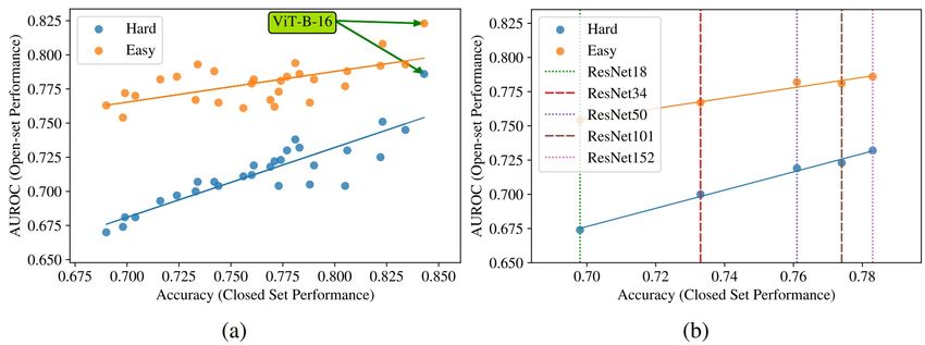
Under review as submission to TMLR

                                                          n
                                        1 2  1 X
                                 min kwk +       ξi − ρ
                                 w,ρ,ξi 2   vn 1
                                                                                                          (1)
                                subject to (w · Φ(xi )) > ρ − ξi , i ∈ 1, ..., n
                                                  ξi > 0, i ∈ 1, . . . , n

Finding a hyper-plane appears to be a brilliant approach for imposing a shared normal restriction on the
training samples. But unfortunately, because half-space is not compact enough to grasp unique shared
normal features, it generates a large number of false negatives. Therefore, similarly, Support Vector Data
Description(SVDD) tries to find the most compact hyper-sphere that includes normal training samples. This
is much tighter than a hyper-plan, thus finds richer normal features, and is more robust against unwanted
noises as Eq. 2 shows. Both of the mentioned methods offer soft and hard margin settings, and in the former,
despite the latter, some samples can cross the border and remain outside of it even if they are normal. OC-
SVM has some implicit assumptions too; for example, it assumes training samples obey a shared concept,
which is conceivable due to the one-class setting. Also, it works pretty well on the AD setting in which the
number of outliers is significantly lower than normal ones however fails on high dimensional datasets.

                                      n
                                      X
                              min C         ξi + R 2
                               R,a
                                      i=1
                                                              2
                                                                                                          (2)
                              subject to      kφ(xi ) − ak 6 R2 + ξi , i ∈ 1, . . . , n
                                               ξi > 0, i ∈ 1, . . . , n

4     Anomaly and Novelty Detection
Anomaly Detection (AD) and Novelty Detection (ND) have been used interchangeably in the literature,
with few works addressing the differences Perera et al. (2019); Xia et al. (2015); Wang et al. (2019). There
are specific inherent challenges with anomaly detection that contradict the premise that the training data
includes entirely normal samples. In physical investigations, for example, measurement noise is unavoidable;
as a result, algorithms in an unsupervised training process must automatically detect and focus on the
normal samples. However, this is not the case for novelty detection problems. There are many applications
in which providing a clean dataset with minimum supervision is an easy task. While these domains have
been separated over time, their names are still not appropriately used in literature. These are reviewed here
in a shared section.
Interests in anomaly detection go back to 1969 Grubbs (1969), which defines anomaly/outlier as “samples
that appear to deviate markedly from other members of the sample in which it occurs", explicitly
assuming the existence of an underlying shared pattern that a large fraction of training samples follow. This
definition has some ambiguity. For example, one should define a criterion for the concept of deviation or
make the term “markedly" more quantitative.
To this end, there has been a great effort both before and after the advent of deep learning methods to make
the mentioned concepts more clear. To find a sample that deviates from the trend, adopting an appropriate
distance metric is necessary. For instance, deviation could be computed in a raw pixel-level input or in a
semantic space that is learned through a deep neural network. Some samples might have a low deviation from
others in the raw pixel space but exhibit large deviations in representation space. Therefore, choosing the
right distance measure for a hypothetical space is another challenge. Finally, the last challenge is choosing
the threshold to determine whether the deviation from normal samples is significant.

4.1   Anomaly Detection With Robust Deep Auto-encoders Zhou & Paffenroth (2017):

This work trains an AutoEncoder (AE) on a dataset containing both inliers and outliers. The outliers are
detected and filtered during training, under the assumption that inliers are significantly more frequent and

                                                           8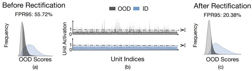
Under review as submission to TMLR
have a shared normal concept. This way, the AE is trained only on normal training samples and consequently
poorly reconstructs abnormal test time inputs. The following objective function is used:
min ||LD − Dθ (Eθ (LD ))||2 + λ||S||1
θ
(3)
s.t. X − LD − S = 0,
where E and D are encoder and decoder networks, respectively. LD is the inlier part and S the outlier part
of the training data X. However, the above optimization is not easily solvable since S and θ need to be
optimized jointly. To address this issue, the Alternating Direction Method of Multipliers (ADMM) is used,
which divides the objective into two (or more) pieces. At the first step, by fixing S, an optimization problem
on the parameters θ is solved such that LD = X − S, and the objective is ||LD − Dθ (Eθ (LD ))||2 . Then
by setting LD to be the reconstruction of the trained AE, the optimization problem on its norm is solved
when S is set to be X − LD . Since the L1 norm is not differentiable, a proximal operator is employed as an
approximation of each of the optimization steps as follows:
x i − λ
xi > λ
proxλ,L1 (xi ) = xi + λ xi < −λ (4)
0
− λ ≤ xi ≤ λ
Such a function is known as a shrinkage operator and is quite common in L1 optimization problems. The
mentioned objective function with ||S||1 separates only unstructured noises, for instance, Gaussian noise
on training samples, from the normal content in the training dataset. To separate structured noises such
as samples that convey completely different meaning compared to the majority of training samples, L2,1
optimization norm can be applied as:
n
X n X
X m
||xj ||2 = ( |xij |2 )1/2 , (5)
j=1 j=1 i=1
with a proximal operator that is called block-wise soft-thresholding function Mosci et al. (2010). At the test
time, the reconstruction error is employed to reject abnormal inputs.
4.2 Adversarially Learned One-Class Classifier for Novelty Detection (ALOCC) Sabokrou et al.
(2018a):
In this work, it is assumed that a fully normal training sample is given, and the goal is to train a novelty
detection model using them. At first, (R) as a Denoising Auto Encoder (DAE) is trained to (1) decrease
the reconstruction loss and (2) fool a discriminator in a GAN-based setting. This helps the DAE to produce
high-quality images instead of blurred outputs Larsen et al. (2016). This happens because, on the one hand,
the AE model loss explicitly assumes independent Gaussian distributions for each of the pixels. And on the
other hand, true distributions of pixels are usually multi-modal, which forces the means of Gaussians to settle
in between different modes. Therefore, they produce blurry images for complex datasets. To address this
issue, AEs can be trained in a GAN-based framework to force the mean of each of Gaussians to capture just
one mode of its corresponding true distribution. Moreover, by using the discriminator’s output (D) instead
of the pixel-level loss, normal samples that are not properly reconstructed can be detected as normal. This
loss reduces the False Positive Rate (FPR) of the vanilla DAE significantly. The objective function is as
9
Under review as submission to TMLR

follows:

                                  LR+D = min max EX∼pt [log(D(X))]+
                                          R   D

                                       EX∼p
                                        e t +Nσ ([log(1 − D(R( X)))]
                                                               e                                           (6)

                                  LR = ||X − X 0 ||2
                                  L = LR+D + LR ,

where X 0 is the reconstructed output of the decoder, and pt is the distribution of the target class (i.e.,
normal class). This helps the model to not only have the functionality of AEs for anomaly detection but
also produces higher quality outputs. Furthermore, detection can be done based on D(R(X)) as mentioned
above. Fig. 5 depicts the overall architecture of this work.
An extended version of ALOCC, where the R(X) network has been formed as a Variational AE is presented
in Sabokrou et al. (2020). Besides, the ALOCC can not process the entire input data (images or video
frames) at one step and needs the test samples to divide into several patches. Processing the patches makes
the method computationally expensive. To address this problem, AVID Sabokrou et al. (2018b) was proposed
to exploit a fully convolutional network as a discriminator (i.e., D) to score (and hence detect) all abnormal
regions in the input frame/image all at once.

Figure 5: An overview of the ALOCC method is shown. This work trains an autoencoder that fools a
discriminator in a GAN-based setting. This helps the AE to make high-quality images instead of blurred
outputs. Besides, by using the discriminator’s output, a more semantic similarity loss is employed instead
of the pixel-level L2 reconstruction loss.

4.3   One-Class Novelty Detection Using GANs With Constrained Latent Representations (OC-GAN)
      Perera et al. (2019):

As one of the challenges, AE trained on entirely normal training samples could reconstruct unseen abnormal
inputs with even lower errors. To solve this issue, this work attempts to make the latent distribution of the
encoder (EN(·)) similar to the uniform distribution in an adversarial manner:

                                   llatent     = −(Es∼U(−1,1) [log(Dl (s))]+
                                                                                                           (7)
                                             Ex∼px [log(1 − Dl (EN(x+n)))]),

where n ∼ N (0, 0.2), and Dl is the latent discriminator. The discriminator forces the encoder to produce
uniform distribution on the latent space. Similarly, the decoder (De(·)) is forced to reconstruct in-class
outputs for any latent value sampled from the uniform distribution as follows :

                                                       10
Under review as submission to TMLR
lvisual = −(Es∼U(−1,1) [log(Dv (De(s)))]+
(8)
Ex∼pl [log(1 − Dv (x))]),
where Dv is called visual discriminator.
Intuitively, the learning objective distributes normal features in the latent space such that the reconstructed
outputs entirely or at least roughly resemble the normal class for both normal and abnormal inputs. Another
technique called informative negative sample mining is also employed on the latent space to actively seek
regions that produce images of poor quality. To do so, a classifier is trained to discriminate between the
reconstructed outputs of the decoder and fake images, which are generated from randomly sampled latent
vectors. To find informative negative samples, the algorithm (see Fig. 6) starts with a random latent-space
sample and uses the classifier to assess the quality of the generated image. After that, the algorithm solves
an optimization in the latent space to make the generated image such that the discriminator detects it as
fake. Finally, the negative sample is used to boost the training process.
As in previous AE-based methods, reconstruction loss is employed in combination with the objective above.
Reconstruction error is used as the test time anomaly score.
Figure 6: The training process of OC-GAN method Perera et al. (2019).
4.4 Latent Space Autoregression for Novelty Detection (LSA) Abati et al. (2019):
This work proposes a concept called "surprise" for novelty detection, which specifies the uniqueness of input
samples in the latent space. The more unique a sample is, the less likelihood it has in the latent space,
and subsequently, the more likely it is to be an abnormal sample. This is beneficial, especially when there
are many similar normal training samples in the training dataset. To minimize the MSE error for visually
identical training samples, AEs often learn to reconstruct their average as the outputs. This can result in
fuzzy results and large reconstruction errors for such inputs. Instead, by using the surprise loss in combination
with the reconstruction error, the issue is alleviated. Besides, abnormal samples are usually more surprising,
and this increases their novelty score. Surprise score is learned using an auto-regressive model on the latent
space, as Fig. 7 shows. The auto-regressive model (h) can be instantiated from different architectures,
11Under review as submission to TMLR
such as LSTM and RNN networks, to more complex ones. Also, similar to other AE-based methods, the
reconstruction error is optimized. The overall objective function is as follows:
L = LRec (θE , θD ) + λ · LLLK (θE , θh )
(9)
= EX ||x − x̂||2 − λ · log(h(z; θh ))
Figure 7: An overview of the LSA method is shown. A surprise score is defined based on the probability
distribution of embeddings. The probability distribution is learned using an auto-regressive model. Also,
reconstruction error is simultaneously optimized on normal training samples.
4.5 Memory-Augmented Deep Autoencoder for Unsupervised Anomaly Detection (Mem-AE) Gong
et al. (2019):
This work challenges the second assumption behind using AEs. It shows that some abnormal samples could
be perfectly reconstructed even when there are not any of them in the training dataset. Intuitively, AEs
may not learn to extract uniquely describing features of normal samples; as a result, they may extract
some abnormal features from abnormal inputs and reconstruct them perfectly. This motivates the need
for learning features that allow only normal samples to be reconstructed accurately. To do so, Mem-AE
employs a memory that stores unique and sufficient features of normal training samples. During training,
the encoder implicitly plays the role of a memory address generator. The encoder produces an embedding,
and memory features that are similar to the generated embedding are combined. The combined embedding
is then passed to a decoder to make the corresponding reconstructed output. Also, Mem-AE uses a sparse
addressing technique that uses only a small number of memory items. Accordingly, the decoder in Mem-AE
is restricted to performing the reconstruction using a small number of addressed memory items, rendering
the requirement for efficient utilization of the memory items. Furthermore, the reconstruction error forces
the memory to record prototypical patterns that are representative of the normal inputs. To summarize the
training process, Mem-AE (1) finds address Enc(x) = z from the encoder’s output; (2) measures the cosine
similarity d(z, mi ) of the encoder output z with each of the memory elements mi ; (3) computes attention
weights w, where each of its elements is computed as follows:
exp(d(z, mi ))
wi = PN ; (10)
j=1 exp(d(z, mj ))
(4) applies address shrinkage techniques to ensure sparsity:
max(wi − λ, 0).wi
ŵi = (11)
|wi − λ| +
12Under review as submission to TMLR
T
X
E(ŵt ) = −ŵi . log(ŵi ), (12)
i=1
and finally, the loss function is defined as (13), where R is the reconstruction error and is used as the test
time anomaly score. Fig. 8 shows the overview of architecture.
T
1X
L(θe , θd , M ) = R(xt , x̂t ) + αE(ŵt ) (13)
T t=1
Figure 8: An overview of the Mem-AE method is shown. Each sample is passed through the encoder, and a
latent embedding z is extracted. Then using the cosine similarity, some nearest learned normal features are
selected from the memory, and the embedding ẑ is made as their weighted average. At last, the reconstruction
error of the decoded ẑ and input is considered as the novelty score.
4.6 Redefining the Adversarially Learned One-Class Classifier Training Paradigm (Old-is-Gold) Zaheer
et al. (2020):
This work extends the idea of ALOCC Sabokrou et al. (2018a). As ALOCC is trained in a GAN-based
setting, it suffers from stability and convergence issues. On one hand, the over-training of ALOCC can
confuse the discriminator D because of the realistically generated fake data. On the other hand, under-
training detriments the usability of discriminator features. To address this issue, a two-phase training
process is proposed. In the first phase, a similar training process as ALOCC is followed :
L = LR+D + LR (14)
As phase one progresses, a low-epoch generator model G old for later use in phase two of the training is saved.
The sensitivity of the training process to the variations of the selected epoch is discussed in the paper.
During the second phase, samples X̂ = G are considered high-quality reconstructed data. Samples X̂ low =
G old (X) are considered as low-quality samples. Then, pseudo anomaly samples are created as follows:
ˆ = G (Xi ) + G (Xj )
old old
X̄
2 (15)
X̂ pseudo ˆ
= G(X̄ )
13Under review as submission to TMLR
After that, the discriminator is trained again to strengthen its features by distinguishing between good
quality samples such as {X, X̂} and low-quality or pseudo anomaly ones such as {X̂ low , X̂ pseudo } as follows:
max α · EX [log(1 − D(X))] + (1 − α) · EX̂ [log(1 − D(X̂))]
D
+ (β · EX̂ low [log(1 − D(X̂ low ))] (16)
+ (1 − β) · EX̂ pseudo [log(1 − D(X̂ pseudo ))]
Figure 9: An overview of the Old-Is-Gold method is shown. The architecture is similar to ALOCC; however,
it saves the weights of the network G during the training process, which are called Gold . Then, Gold is
employed to make some low-quality samples that the discriminator is expected to distinguish as normal.
Also, some pseudo abnormal samples are generated by averaging each pair of normal low-quality samples,
which the discriminator is supposed to distinguish as fake inputs. This makes the discriminator’s features
rich and stabilizes the training process.
In this way, D does not collapse as in ALOCC, and D(G(X)) is used as the test time criterion. Fig. 9 shows
the overall architecture of this method.
4.7 Adversarial Mirrored Autoencoder (AMA) Somepalli et al. (2020):
The overall architecture of AMA is similar to ALOCC. However, it challenges the first assumption of AEs.
It has been shown that lp norms are not suitable for training AEs in the anomaly detection domain since
they cause blurry reconstructions and subsequently increase the error of normal samples. To address this
problem, AMA proposes to minimize the Wasserstein distance between distributions PX,X and PX,X̂ . The
objective function is as follows:
W (PX,X , PX,X̂ ) = max Ex∼PX [D(X, X) − D(X, X̂)] (17)
D∈Lip−1
where X̂ is the reconstructed image.
Berthelot et al. (2018) showed that by forcing the linear combination of latent codes of a pair of data points
to look realistic after decoding, the encoder learns a better representation of data. Inspired by this, AMA
makes use of X̂inter —obtained by decoding the linear combination of some randomly sampled inputs:
min max Ex∼PX [D(X, X) − D(X, X̂inter )] (18)
G D∈Lip−1
14Under review as submission to TMLR
To further boost discriminative abilities of D, inspired by Choi & Jang (2018), normal samples are supposed
as residing in the typical set Cover & Thomas (2006) while anomalies reside outside of it, a Gaussian
regularization equal to L2 norm is imposed on the latent representation. Then using the Gaussian Annulus
Theorem Vershynin√ (2018) stating that in a d-dimensional space, the typical set resides with high probability
at a distance of d from the origin, synthetic negatives (anomalies), are obtained by sampling the latent
space outside and closer to the typical set boundaries. Therefore, the final objective function is defined as
follows:
min max Lnormal − λneg · Lneg
G D∈Lip−1
h
Lnormal = Ex∼PX D(X, X) − D(X, X̂)
i (19)
+ λinter · (D(X, X) − D(X, X̂inter )) + λreg · kE(X)k
h i
Lneg = Ex∼e QX
D(X, X) − D(X, X̂ neg )
Fig. 10 shows an overview of the method and the test time criterion is ||f (X, X) − f (X, G(E(X))||1 where
f is the penultimate layer of D.
Figure 10: An overview of AMA method is shown. The architecture is similar to ALOCC; however, it does not
try to minimize reconstruction error between x and x̂. Instead, a discriminator is trained with Wasserstein
Loss to minimize the distance between the distribution (x, x) and (x, x̂). In this way, it forces x̂ to be similar
to x without using any lp norm that causes blurred reconstructed outputs. Moreover, some negative latent
vectors are sampled from low probability areas, which the discriminator is supposed to distinguish as fake
ones. This makes the latent space consistent compared to the previous similar approaches.
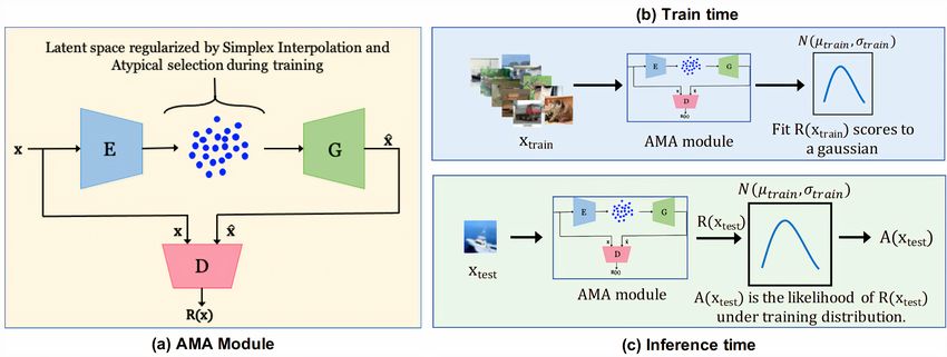
4.8 Unsupervised Anomaly Detection with Generative Adversarial Networks to Guide Marker
Discovery (AnoGAN) Schlegl et al. (2017):
This work trains a GAN on normal training samples, then at the test time, solves an optimization problem
that attempts to find the best latent space z by minimizing a discrepancy. The discrepancy is found by using
a pixel-level loss of the generated image and input in combination with the loss of discriminator’s features
at different layers when the generated and input images are fed. Intuitively, for normal test time samples, a
desired latent vector can be found despite abnormal ones. Fig. 11 shows the structure of the method.
As inferring the desired latent vector through solving an optimization problem is time-consuming, some
extensions of AnoGAN have been proposed. For instance, Efficient-GAN Zenati et al. (2018) tries to sub-
stitute the optimization problem by training an encoder E such that the latent vectors z 0 approximate the
distribution of z. In this way, E is used to produce the desired latent vector, significantly improving test
time speed. Fig. 12 shows the differences. The following optimization problem (20) is solved at the test
time to find z. The anomaly score is assigned based on how well the found latent vector can minimize the
objective function.
15Under review as submission to TMLR
X X
min (1 − λ) · |x − G(z)| + λ · |D(x) − D(G(z))| (20)
z
Figure 11: An overview of AnoGAN method. At first, a generator network G and a discriminator D are
trained jointly on normal training samples using the standard training loss, which yields a semantic latent
representation space. Then at the test time, an optimization problem that seeks to find an optimal latent
embedding z that mimics the pixel-level and semantic-level information of the input is solved. Intuitively,
for normal samples, a good approximation of inputs can be found in the latent space; however, it is not
approximated well for abnormal inputs.
Figure 12: Figure A shows the architecture of AnoGAN. Figure B shows the architecture of Efficient-GAN.
The encoder E mimics the distribution of the latent variable z. The discriminator D learns to distinguish
between joint distribution of (x, z) instead of x.
4.9 Deep One-Class Classification (DeepSVDD) Ruff et al. (2018):
This method can be seen as an extension of SVDD using a deep network. It assumes the existence of
shared features between training samples, and tries to find a latent space in which training samples can be
compressed into a minimum volume hyper-sphere surrounding them. Fig. 13 shows the overall architecture.
The difference w.r.t traditional methods is the automatic learning of kernel function φ by optimizing the
parameters W . To find the center c of the hyper-sphere, an AE is first trained on the normal training
samples, then the average of normal sample latent embeddings is considered as c. After that, by discarding
the decoder part, the encoder is trained using the following objective function:
n L
1X λX
min ||φ(xi ; W ) − c||22 + ||W l ||2F , (21)
W n i=1 2
l=1
16Under review as submission to TMLR
where W l shows the weights of encoder’s lth layer. At the test time, anomaly score is computed based on
||φ(x; W ∗ ) − c||2 where W ∗ denotes trained parameters.
Figure 13: An overview of the DSVDD method is shown. It finds a minimum volume hyper-sphere that
contains all training samples. As the minimum radius is found, more distance to the center is expected for
abnormal samples compared to normal ones.
4.10 Deep Semi-Supervised Anomaly Detection Ruff et al. (2019):
This is the semi-supervised version of DSVDD which assumes a limited number of labeled abnormal samples.
The loss function is defined to minimize the distance of normal samples from a pre-defined center of a hyper-
sphere while maximizing abnormal sample distances. The objective function is defined as follows:
n
1 X
min ||φ(xi ; W ) − c||2 +
W n + m i=1
m L
(22)
η X λX
(||φ(x̂i ; W ) − c||2 )yˆj + ||W l ||2F
n + m j=1 2
l=1
Note that, as mentioned above, there is access to (xˆ1 , yˆ1 ), ..., (xˆm , yˆm ) ∈ X × Y with Y = {−1, +1} where
ŷ = 1 denotes known normal samples and ŷ = −1 otherwise. c is specified completely similar to DSVDD
by averaging on the latent embeddings of an AE trained on normal training samples. From a somewhat
theoretical point of view, AE’s objective loss function helps the encoder maximize I(X; Z) in which X denotes
input variables and Z denotes latent variables. Then, it can be shown that (22) minimizes the entropy of
normal sample latent embeddings while maximizing it for abnormal ones as follows:
Z
H(Z) = E[− log(P (Z)] = − p(z) log p(z) dz
Z (23)
1
≤ log((2πe)d det(Σ)) ∝ log σ 2
2
As the method makes normal samples compact, it forces them to have low variance, and consequently, their
entropy is minimized. The final theoretical formulation is approximated as follows:
max I(X; Z) + β(H(Z − ) − H(Z + )) (24)
p(z|x)
4.11 Deep Anomaly Detection Using Geometric Transformations (GT) Golan & El-Yaniv (2018):
GT attempts to reformulate the one-class classification problem into a multi-class classification. GT defines a
set of transformations that do not change the data distribution, then trains a classifier to distinguish between
17Under review as submission to TMLR
them. Essentially, the classifier is trained in a self-supervised manner. Finally, a Dirichlet distribution
is trained on the confidence layer of the classifier to model non-linear boundaries. Abnormal samples are
expected to be in low-density areas since the network can not confidently estimate the correct transformation.
At the test time, different transformations are applied to the input, and the sum of their corresponding
Dirichlet probabilities is assigned as the novelty score. An overview of the method is shown in Fig. 14.
Figure 14: An overview of the GT method is shown. A set of transformations is defined, then a classifier must
distinguish between them. Having trained the classifier in a self-supervised manner, a Dirichlet distribution
is trained on the confidence layer to model their boundaries.
4.12 Effective End-To-End Unsupervised Outlier Detection via Inlier Priority of Discriminative
Network Wang et al. (2019):
In this work, similar to GT, a self-supervised learning (SSL) task is employed to train an anomaly detector
except in the presence of a minority of outliers or abnormal samples in the training dataset. Suppose the
following training loss is used as the objective function:
K
1 X (y)
LSS (xi | θ) = − log(P (y) (xi | θ)), (25)
K y=1
(y)
where xi is obtained by applying a set of transformations O(. | y), and y indicates each transformation.
The anomaly detection is obtained based on the objective function score. Take for example the rotation
prediction task. During training, the classifier learns to predict the amount of rotation for normal samples.
During test time, different rotations are applied on inputs, the objective function scores for normal samples
would be lower than abnormal ones.
However, due to the presence of abnormal samples in the training dataset, the objective score for abnormal
samples may not always be higher. To address this issue, it is shown that the magnitude and direction of
gradient in each step have a significant tendency toward minimizing inlier samples’ loss function. Thus the
network produces lower scores compared to abnormal ones. Wang et al. (2019) exploits the magnitude of
(in) (out)
transformed inliers and outliers’ aggregated gradient to update wc , i.e. ||∇wc L|| and ||∇wc L||, which are
shown to follow this approximation:
(in)
E(||∇wc · L||2 ) 2
Nin
(out)
≈ 2 (26)
E(||∇wc · L||2 ) Nout
18Under review as submission to TMLR
where E(·) denotes the probability expectation. As Nin
Nout , normal samples have more effect on the
training procedure. Also, by projecting and averaging the gradient in the direction of each of the training
−∇θ L(xi )
sample’s gradient (−∇θ L(x) · ||−∇ θ L(xi )||
), the stronger effect of inlier distribution vs outlier is observed
again. Fig. 15 shows the effect empirically.
Figure 15: The average magnitude of the gradient for inliers and outliers with respect to the number of
iterations. The class used as inliers is in brackets.
4.13 Classification-Based Anomaly Detection for General Data (GOAD) Bergman & Hoshen (2020):
This work is very similar to GT. It trains a network to classify between different transformations; however,
instead of using cross-entropy loss or training a Dirichlet distribution on the final confidences, it finds a
center for each transformation and minimizes the distance of each transformed data with its corresponding
center as follows :
2
e−||f (T (x,m))−cm0 ||
P (m0 | T (x, m)) = P −||f (T (x,m))−c ||2 (27)
m̂ e
m̂
where thePcenters cm are given by the average feature over the training set for every transformation i.e.
cm = N1 x∈X f (T (x, m)). For training f , two options are used. The first one is using a simple cross
entropy on P (m0 | T (x, m)) values, and the second one is using the center triplet loss He et al. (2018) as
follows:
X
max(0, ||f (T (xi , m)) − cm ||2 + s
i (28)
− min
0
||f (T (xi , m)) − cm0 ||2 )
m 6=m
where s is a margin regularizing the distance between clusters.
The idea can be seen as the combination of DSVDD and GT in which GT’s transformations are used, and
different compressed hyperspheres are learned to separate them. M different transformations transform each
sample at the test time, and the average of correct label probabilities is assigned as the anomaly score.
4.14 CSI: Novelty Detection via Contrastive Learning on Distributionally Shifted Instances Tack
et al. (2020):
This work attempts to formulate the problem of novelty detection into a contrastive framework similar to
SimCLR Chen et al. (2020b). The idea of contrastive learning is to train an encoder fθ to extract the
necessary information to distinguish similar samples from others. Let x be a query, x+ , and x− be a set of
positive and negative samples respectively, z be the encoder’s output feature or the output of an additional
projection layer gφ (fθ (x)) for each input, and suppose sim(z, z 0 ) is cosine similarity. Then, the primitive
form of the contrastive loss is defined as follows:
19You can also read