A method of defect depth estimation for simulated infrared thermography data with deep learning

Preprints (www.preprints.org) | NOT PEER-REVIEWED | Posted: 22 March 2021 doi:10.20944/preprints202008.0565.v2

 Peer-reviewed version available at Appl. Sci. 2020, 10, 6819; doi:10.3390/app10196819

 Article

 A method of defect depth estimation for simulated
 infrared thermography data with deep learning
 Qiang Fang1*, Farima. Abdolahi. Mamoudan1, Xavier. Maldague 1,*
 1 Computer Vision and Systems Laboratory, Department of Electrical and Computer Engineering,
 Université Laval, 1065, av. de la Médecine, Québec (QC), Canada, G1V 0A6; qiang.fang.1@ulaval.ca;
 * Correspondence: qiang.fang.1@ulaval.ca (Q.F.); Xavier.Maldague@gel.ulaval.ca (X.M.);

 Received: 25 August 2020 / Revised: 21 September 2020 / Accepted: 25 September 2020 / Published: 29
 September 2020

 Abstract: Infrared thermography has already been proven to be a significant method in non-
 destructive evaluation since it gives information with immediacy, rapidity, and low cost. However,
 the thorniest issue for the wider application of IRT is quantification. In this work, we proposed a
 specific depth quantifying technique by employing the Gated Recurrent Units (GRU) in composite
 material samples via pulsed thermography (PT). Finite Element Method (FEM) modeling provides
 the economic examination of the response pulsed thermography. In this work, Carbon Fiber
 Reinforced Polymer (CFRP) specimens embedded with flat bottom holes are stimulated by a FEM
 modeling (COMSOL) with precisely controlled depth and geometrics of the defects. The GRU model
 automatically quantified the depth of defects presented in the stimulated CFRP material. The
 proposed method evaluated the accuracy and performance of synthetic CFRP data from FEM for
 defect depth predictions.

 Keywords: NDT Methods; Defects depth estimation; Pulsed thermography; Gated Recurrent Units

 1. Introduction
 Non-destructive evaluation (NDE) has emerged as an important method for the evaluation of
 the properties of components or systems without damaging their structure. Several state of the arts
 methodologies such as Pulsed Phase Thermography (PPT) [1], Principal Component Thermography
 (PCT) [2], Differential of Absolute Contrast (DAC) [3], Thermographic Signal Reconstruction
 (TSR)[4], as well as Candid Covariance Free Incremental Principal Component Thermography [5],
 have been implemented to process thermographic sequences and improve the defect visibility. These
 techniques can be beneficial for qualitative analysis of composite materials. However, to introduce a
 method for conducting quantitative study (defect depth estimation) with deep learning is a novel
 topic to be explored.
 Quantitative analysis is playing an important role in the modern industrial field of Non-
 destructive testing (NDT). Defect characterization is one of the current topics of interest in
 quantitative data analysis of active thermography. In this topic, thermographic information involves
 extracting quantitative subsurface properties from defects such as defect depth, lateral size, thermal
 resistivity, from an experimental Thermal Non-destructive Testing (TNDT) dataset utilized to
 characterize defects. Several approaches have already been proposed to analyze the depth in the
 region of defects in pulsed thermography. In general, these approaches evaluate the defects depth by
 using the maximum thermal contrast C_max, the instant of maximum thermal contrast Tc_max or
 artificial neural networks to analyze the depth of defects based on mathematical equations. The Peak
 Temperature Contrast Method [6] estimated the depth based on the characteristic time from peak
 contrast. The peak contrast corresponding to the maximum contrast has a proportional correlation

 Appl. Sci. 2020, 10, x; doi: FOR PEER REVIEW www.mdpi.com/journal/applsci

 © 2021 by the author(s). Distributed under a Creative Commons CC BY license.

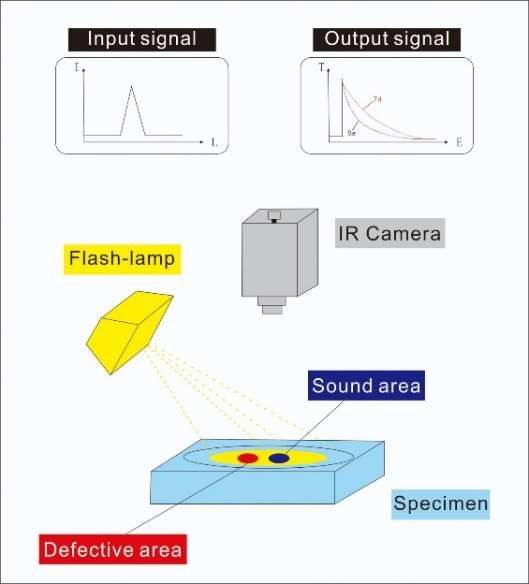
Preprints (www.preprints.org) | NOT PEER-REVIEWED | Posted: 22 March 2021 doi:10.20944/preprints202008.0565.v2

 Peer-reviewed version available at Appl. Sci. 2020, 10, 6819; doi:10.3390/app10196819

 Appl. Sci. 2020, 10, x FOR PEER REVIEW 2 of 13

 with the square of the defect depth. A. Daribi, et al. [7] proposed neural networks for defect
 characterization of defect depth. The results demonstrated that the networks should be trained by
 representative and non-redundant data in order to obtain a high degree of classification accuracy.
 In this work, there is an attempt to detect the depth of defects in carbon fiber reinforced polymer
 (CFRP) via Gated Recurrent Units (GRU) [17]. GRU is an updated recurrent neural network (RNN)
 particularly designed for time series prediction. GRU can be considered as a variation of Long Short-
 Term Memory (LSTM) [18]. Compared with the LSTM and RNN temporal model, the GRU has
 adapted a few learning parameters which could save computational expenses for training and
 obtained an excellent performance. According to our knowledge, this is the first time that the thermal
 temporal characteristic model (GRU; RNN; LSTM etc.) is used to qualify the depth of defects.
 We modeled a 3D version of CFRP specimen stimulation from COMSOL. Then, it was further
 tested on the systemic data by the GRU model to validate its accuracy. The remainder of this paper
 is structured as follows: section 2 provides the pulsed thermography theory and conception
 indication, as well as the detailed characteristics of FEM simulations. Section 3 proposed a GRU
 model-based defects depth estimation strategy and introduces the GRU deep learning model
 architectures. Section 4 provides the experimental results analysis. Section 5 concludes this paper.

 2. Thermal Consideration and FEM Stimulation

 2.1. Pulsed thermography
 In pulsed thermography, a high-power exponential heating impulse is applied to the samples,
 and a thermal response is measured during a period of time. Due to the heat conduction, a surface
 region which has an internal defect underneath the surface perturbs the thermal waves propagation
 on the surface of specimens in comparison to the sound (non-defective) region. We can then see the
 changes of the temperature variation, since the internal defects possess different thermo-physical
 (conductivity, density and heat capacity) that have an impact on heat flow. These thermal differences
 can be observed as surface features and recorded with an infrared camera as indicated in Figure 1 [8].
 Temporal evolutions can be observed from the defective regions and subsurface sound regions.
 A thermal contrast is acquired as a feature vector which is obtained distinctly via the thermal value
 from the defective region subtracted from the corresponding value from the surrounding sound
 region [9] as indicated in Eq (1), where Td(t) is the temperature value on the pixel point of the defect
 area. The temperature value on the reference point of the sound area is ( ) Then the (t) is the
 absolute thermal contrast extracted from the defect and sound region. The thermal contrast is an
 excellent technique to distinguish the temperature difference to learn the depth of the defects, as
 shown in Figure 1.

 ( )= ( ) − ( ) (1)

 2.2. Finite element modeling with transient heat transfer
 Finite Element Modelling (FEM: COMSOL, etc.) [10] has become an important and economical
 platform to evaluate the thermal response of pulsed thermography, which builds up models for the
 platform of components that allow us to flexibly examine all specific physical aspects of thermal data
 such as geometries and properties of materials. Simulated thermograms matched well with
 experimental data.
 In this work, COMSOL will be utilized as a 3D based simulation to build up models for the
 synthetic data to provide for depth estimation of artificial defects. A Carbon Fiber Reinforced
 Polymer (CFRP) structure-based specimen containing artificial defects of different shapes (flat-
 bottom holes) is modeled as shown in Figure 2. A high thermal pulse is projected on the surface of
 specimens. Due to the existence of the temperature gradients in the sample, a thermal front
 propagates from the high temperature region on the surface to the region underneath. A
 delamination or discontinuities create a lower thermal diffusion rate to the heat flow and then reflect
 the unnormal thermal patterns on the surface. The COMSOL software is utilized as the heat transfer

Preprints (www.preprints.org) | NOT PEER-REVIEWED | Posted: 22 March 2021 doi:10.20944/preprints202008.0565.v2

 Peer-reviewed version available at Appl. Sci. 2020, 10, 6819; doi:10.3390/app10196819

 Appl. Sci. 2020, 10, x FOR PEER REVIEW 3 of 13

 simulation model for obtaining the temperature evaluations of the surface of each sample, as
 indicated below [11]:

 ( ) − ∙ ( )=0 (2)

 + + = (3)

 ∙ ( ∙ ) = ℎ ( − ) + ( − ) (4)

 where in Equation (2)-(4), the density is ( ) , constant specific heat is ( ) , and the
 .
 absolute temperature is T(K). Time variable is set as t(s). A rectangular coordinate system (x, y, z) as
 in Eq. (3) in anisotropic media can lead to numerous possible solutions. w, , , ( . ) are the
 main conductivity rates and conductivity rates which respectively for three coordinates (x, y, z) in 3D
 thermal modeling. The convection heat transfer is given by ℎ ( ). In Equation (4), a boundary
 condition that regarding to the thermal heat transfer from radiation and convection between the all
 the specimen surfaces and the ambient temperature has been indicated, where is an initial
 environment temperature which consider all the external environment as the same
 temperature; ( ) is the Stefan-Boltzmann physical constant which links the temperature with
 energy ; ε represents surface emissivity.

 Table 1 briefly illustrates the physical properties of CFRP specimens and pulsed thermography
 parameters involved in the COMSOL simulation in this experiment. Table 2 and Table 3 provide the
 description of defect characteristics including the depth, size, shape of each defects, which
 characterized respectively two different group samples for training and testing. The training group
 has 6 CFRP samples (30 cm×30cm). Each sample has a different geometric distribution, depth, and
 size of defects.
 Each row in every CFRP samples has the same depth of defect, which included 22 different
 constant values from 0.5 mm to 2.2 mm to be set from the first row in training sample 1 to the last
 row in training sample 6. We extracted 5 vectors from each defect region for GRU model training
 with depth estimation. The testing group has 4 CFRP samples (30 cm×30 cm).
 In order to differ from the training samples, the testing group consists of samples A, B, C, D. The
 depth of defects in the test samples range from [0.5mm, 2.2mm] but have a size which differs from
 that of the training samples. The CFRP geometrics of the structure of training sample 1 is indicated
 on Figure 2.

 Figure 1. Pulsed thermographic testing using optical excitation

Preprints (www.preprints.org) | NOT PEER-REVIEWED | Posted: 22 March 2021 doi:10.20944/preprints202008.0565.v2

 Peer-reviewed version available at Appl. Sci. 2020, 10, 6819; doi:10.3390/app10196819

 Appl. Sci. 2020, 10, x FOR PEER REVIEW 4 of 13

 Figure 2. Representative CFRP training sample 1 configuration

 Table 1. Physical properties and parameters of stimulation

 Real
 Sign Parameters in experimental simulation
 value
 Material density 1500
 ε Emissivity 0.90
 C Constant specific heating 1000 .
 L Specimen length 300mm
 W Specimen with 300mm
 H Specimen height 5mm
 End time 9s
 The temperature from initialization 293.15k
 The temperature from ambient 293.15k

 Table 2. Defect characteristics of training samples

 Sample row# Depth(mm) Shape Defect Size (mm)
 1 0.5mm Quadrangle Size = 10; 15; 18
 1 2 0.6mm Round Diameter = 18; 15; 5
 3 0.7mm Quadrangle Size= 5; 10; 18
 1 0.8mm Quadrangle Size= 5; 10; 15
 2 2 0.9mm Round Diameter= 18; 15; 10
 3 1.0mm Quadrangle Size= 5; 15; 18
 1 1.1mm Quadrangle Size= 5; 10; 18
 3 2 1.2mm Round Diameter= 15; 10; 5
 3 1.3mm Quadrangle Size= 10; 15; 18
 1 1.4mm Round Size= 5; 15; 18
 4 2 1.5mm Quadrangle Diameter= 18;10; 5
 3 1.6mm Round Size= 5; 10; 15
 1 1.7mm Round Diameter = 10; 15; 18
 5 2 1.8mm Quadrangle Size= 18; 15; 5
 3 1.9mm Round Diameter= 5; 10; 18
 1 2.0mm Round Diameter= 5; 10 ;15
 6 2 2.1mm Quadrangle Size= 18; 15;10
 3 2.2mm Round Diameter= 5 ;15 ;18

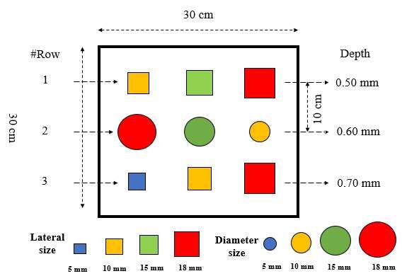
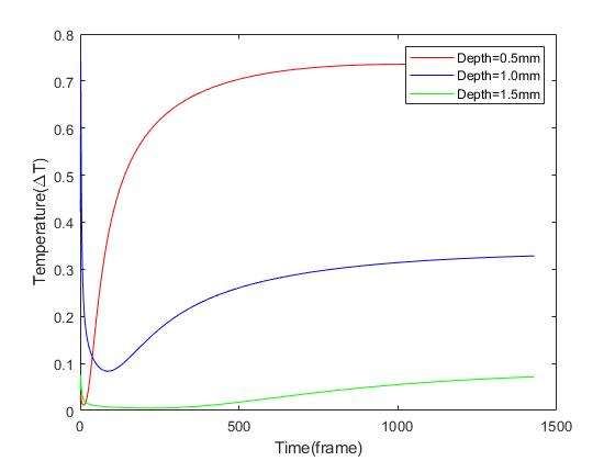
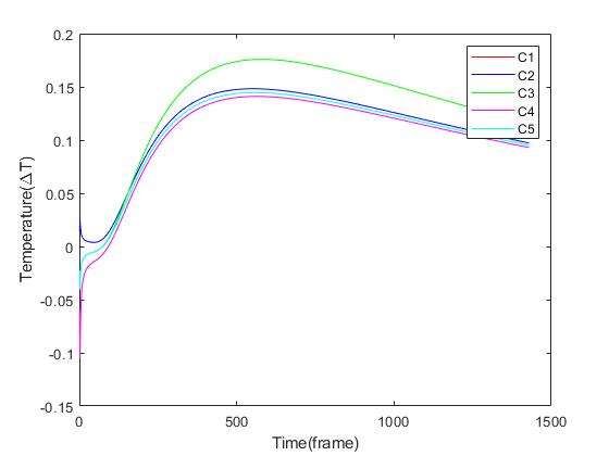
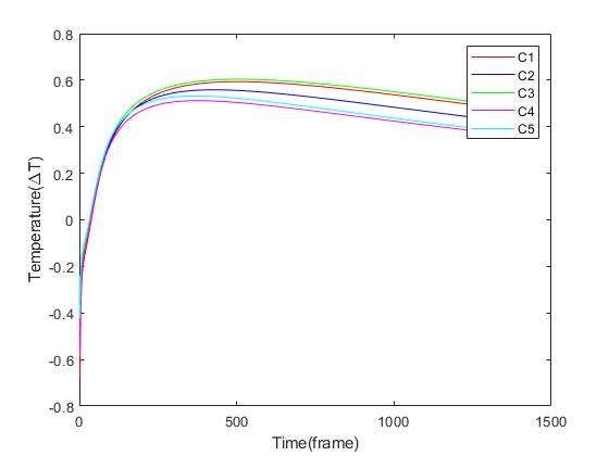
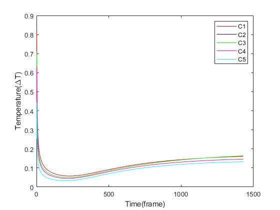
Preprints (www.preprints.org) | NOT PEER-REVIEWED | Posted: 22 March 2021 doi:10.20944/preprints202008.0565.v2

 Peer-reviewed version available at Appl. Sci. 2020, 10, 6819; doi:10.3390/app10196819

 Appl. Sci. 2020, 10, x FOR PEER REVIEW 5 of 13

 Table 3. Defect characteristics of testing samples

 Sample row# Depth (Left; Middle; Right) Shape Defect Size (Left; Middle; Right) (mm)
 1 Depth = 0.5; 0.8; 1.1 Quadrangle Size= 3 ;16 ;13
 A 2 Depth= 0.6; 0.9; 1.2 Round Diameter = 8; 3; 16
 3 Depth= 0.7; 1.0; 1.3 Quadrangle Size= 13; 8; 16
 1 Depth= 1.4; 1.7; 2.0 Quadrangle Size= 8; 3; 16
 B 2 Depth= 1.5; 1.8; 2.1 Round Diameter= 13; 8; 3
 3 Depth= 1.6; 1.9; 2.2 Quadrangle Size= 16; 13; 8
 1 Depth= 0.5; 0.8; 1.1 Round Size= 4; 17; 14
 C 2 Depth= 0.6; 0.9; 1.2 Quadrangle Diameter= 9; 4; 17
 3 Depth= 0.7; 1.0; 1.3 Round Size= 14; 9; 4
 1 Depth= 1.4; 1.7; 2.0 Round Size= 9; 4; 17
 D 2 Depth= 1.5; 1.8; 2.1 Quadrangle Diameter= 14;9;4
 3 Depth= 1.6; 1.9; 2.2 Round Size= 17; 14; 9

 2.3 Temperature and thermal contrast curves

 In transient thermography, previous researchers [6] concluded that the time that
 corresponds to the maximum temperature contrast ∆T has an approximately proportional
 relationship with the square of the depth of the defect (d ). Simultaneously, the proportionality
 coefficient of this relationship rested with the lateral size of the depth: the smaller the defects, the
 lower maximum contrast ∆T and earlier peak time. As indicated in Figure 3, an interesting case is
 highlighted. We observed the temperature evaluation of three defects of the same size
 (18mm×18mm) but different depth such as (0.5 mm,1.0 mm,1.5 mm). Although the three defects have
 the same shape, it can be demonstrated that the shallower the defect, the higher the peak temperature
 value which can be obtained. In Figure 4, the data distribution of the thermal contrast curves is
 illustrated.

 In this work, five contrast vectors have been extracted above each defect region on the surface
 from the different points in the defects (upper left; upper right; center; lower right; lower left; lower
 right) to reduce the inaccurate influences caused by the small temperature variation. Notice that, each
 training sequence to be processed in this work are extracted from the three quarters frames in the
 total frames of the one thermal sequence which already include the information of peak thermal
 contrast ∆ and corresponding _ . As a result, the last quarter frames of thermal curves
 were not extracted in this work which would show a dramatic decrease of the thermal contrasts in
 the graphs. To be notice that, all the thermal sequence stimulated from the COMSOL software based
 on the parameters as indicated on Table 2. All the extraction work was implemented in a program in
 MATLAB software. This partial extraction in thermal data could save the computational expense for
 the training in GRU to some extent.

 A corresponding synthetic thermogram frame for training sample 2 in t=15s generated from
 COMSOL is indicated at in Figure 5 (a); Nine artificial flat bottom Figure 5 (b) hole defects were
 embedded with different depths in the shapes of either circles or squares.

Preprints (www.preprints.org) | NOT PEER-REVIEWED | Posted: 22 March 2021 doi:10.20944/preprints202008.0565.v2

 Peer-reviewed version available at Appl. Sci. 2020, 10, 6819; doi:10.3390/app10196819

 Appl. Sci. 2020, 10, x FOR PEER REVIEW 6 of 13

 Figure 3. Temperature contrast evaluation for defects located at different depths with the same size
 (0.5mm; 1.0mm; 1.5mm) in training samples

 (a) (b)

 (c)
 Figure 4. Data distribution of temperature contrast evaluation for different depths in training samples (a)
 0.5mm; (b) 1.0 mm; (c)1.5mm

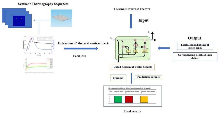
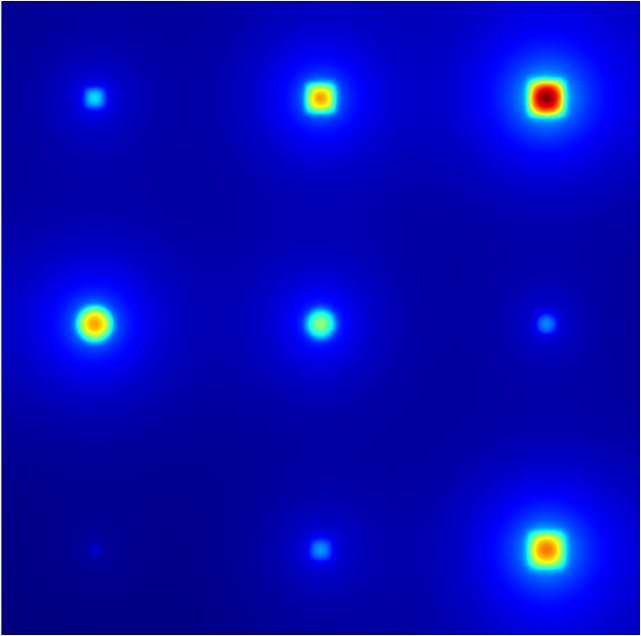
Preprints (www.preprints.org) | NOT PEER-REVIEWED | Posted: 22 March 2021 doi:10.20944/preprints202008.0565.v2

 Peer-reviewed version available at Appl. Sci. 2020, 10, 6819; doi:10.3390/app10196819

 Appl. Sci. 2020, 10, x FOR PEER REVIEW 7 of 13

 (a) (b)
 Figure 5. (a) The corresponding synthetic colorful thermograms in t=15s; (b) 3 D printed defects
 geometrics are highlighted in training samples

 3. Proposed strategy for defect depth estimation

 In this section, a defect depth estimation strategy has been proposed to detect and identify the
 depth of each defect in thermal images as indicated in Figure 6. This design of detection system
 originated from the GRU neural network. The infrared thermal module and simulations are provided
 by COMSOL (FEM simulation) to examine the depth of defects in pulsed thermography (PT). First,
 the synthetic thermal sequences are acquired from FEM (COMSOL) based on the heat transfer
 modeling in FEM. Then, several thermal contrast feature vectors are extracted from each defect region
 to feed into the input of GRU. The output of GRU consists of a unique node which estimated the
 depth during the training. The mean absolute error is chosen as the loss function with the GRU model
 in the equation as below (5). In the end, the predicted depth output from the GRU is based on the
 feature extraction of thermal contrast vectors.

 ∑ ( )
 = (5)

 The GRU takes each vector at a time point in the input. This learning model was trained for 2500
 epochs of each process. The training loss converged to the optimistic value and then flattened. In
 addition, the number of training curves (batch size) is set m. , are the ground truth and estimated
 depth respectively.

Preprints (www.preprints.org) | NOT PEER-REVIEWED | Posted: 22 March 2021 doi:10.20944/preprints202008.0565.v2

 Peer-reviewed version available at Appl. Sci. 2020, 10, 6819; doi:10.3390/app10196819

 Appl. Sci. 2020, 10, x FOR PEER REVIEW 8 of 13

 Figure 6 GRU model-based defects depth estimation strategy

 3.1 Gated recurrent unit model with depth estimator
 Due to the time continuity of the thermal sequence, each frame collected from the experiment is
 related to the recent historical frame, therefore the time series memory deep learning model can be
 applied to the thermography data based on this feature. The GRU model is originally from RNN
 which is a time series model that can handle the continuous information such as thermal sequences
 [12]. During the cooling period of the thermal data, the temperature evaluation curves over time are
 acquired from the given infrared frames. The Learned GRU model is able to distinguish whether the
 pixel is from a defective region or a sound region due to the training period. Therefore, the multiple
 units of GRU could be applied to extract the features of the temperature evaluations from the samples
 based on physical properties.

 The GRU neural network in Figure 7 are structured as follows [13]. In equations (6)-(9), , 
 represent the update, reset gate units respectively. ( ) , ( ) , are the weight factors for each gate
 unit. is the current input. ℎ is the input from the previous time step in the hidden state. ℎ
 ,

 is the input of current memory from the hidden state. ( ) , ( ) , are the weight factors for
 previous time information ℎ [14]. (. ) represents the sigmoid function. ° is denoted as the
 Hadamard product. [16].

 = ( ) ( ) + ( ) (ℎ ) (6)
 = ( ) ( ) + ( ) (ℎ ) (7)
 ,
 ℎ = ℎ ( ) + ° (ℎ ) (8)
 ℎ = ° ℎ + (1 − )° ℎ, (9)

Preprints (www.preprints.org) | NOT PEER-REVIEWED | Posted: 22 March 2021 doi:10.20944/preprints202008.0565.v2

 Peer-reviewed version available at Appl. Sci. 2020, 10, 6819; doi:10.3390/app10196819

 Appl. Sci. 2020, 10, x FOR PEER REVIEW 9 of 13

 Figure 7 Gated Recurrent Unit
 As shown in Figure 8, in this work, the original thermal sequences were reshaped into vectors.
 The particular thermal contrast vectors are directly fed into the input of the GRU network structure.
 Each thermal contrast vector in the defect region is decoded with the depth value of corresponding
 defect at the output of GRU based on the thermal properties from the training sequences. In order to
 select the points for the simulated thermal sequences to extract temperature curves vectors, 5 different
 locations inside each defect surface in these defective areas were selected. Since the temperature of
 the defect region is not even, these selected points accounted for small temperature variations and
 change above each defect surface region. Each thermal contrast vector is vectorized with the same
 length in the time of the thermal sequence. Therefore, the input values of GRU are fed into the
 particular thermal contrast vectors. The output from the decode section (to be connected with the
 fully connected layer) are set with the corresponding defect depth of each vector. The estimated depth
 values in the defect region output from GRU are based on the thermal properties from the training
 sequences.

 Figure 8 The process of GRU depth estimation

Preprints (www.preprints.org) | NOT PEER-REVIEWED | Posted: 22 March 2021 doi:10.20944/preprints202008.0565.v2

 Peer-reviewed version available at Appl. Sci. 2020, 10, 6819; doi:10.3390/app10196819

 Appl. Sci. 2020, 10, x FOR PEER REVIEW 10 of 13

 4 Experimental validation and results

 4.1 Inference and training

 In this research, the training processing on GPU (NVIDIA GeForce GTX 1080Ti) takes about 30
 min. The operating system is set as: Ubuntu 14. 04. CPU: i7-5930k. Memory: 64GB. Adam is
 introduced as optimizer.
 The whole training process was also conducted using the Adam optimization. Some main hyper
 parameters and training parameter are set as below: weight decay - 0.0001, the learning rate 0.001
 and learning momentum 0.9. In this work, the temperature variety and contrast reflect on each vector.
 Therefore, the LSTM time step was set to 1429 (1429 frames as a time step as input).

 4.2 Data Processing
 To reduce the overfitting issue, the cross-validation verification method is proposed in this
 study. First, we collected 270 thermal contrast curves from the simulation data (5 thermal contrast
 curves extracted from each defect averagely). Then, we shuffled all of the data and spilt 80% of the
 data to train with the GRU model, while 20% was utilized to validate the performance of the GRU.
 All obtained training data (the thermal contrast evaluation curves) is normalized and truncated
 as a fixed length of duration. Simultaneously, the input data is normalized by subtracting from the
 mean value of the thermal curves ( ) and dividing by the standard deviation of thermal contrast
 ( ) using Eq. (10).
 ( )
 , ( ) = (10)

 4.3 Depth estimation results and validation
 Table 4. The results of depth estimation of defects located in the designated specimen

 Sample Expected Output(mm) Estimated Output 1(mm) MAE1 Estimated Output 2(mm) MAE2
 AC 0.5 0.522 0.022 0.507 0.007
 AC 0.6 0.604 0.004 0.603 0.003
 AC 0.7 0.708 0.008 0.706 0.006
 AC 0.8 0.814 0.014 0.807 0.007
 AC 0.9 0.912 0.012 0.913 0.013
 AC 1.0 1.041 0.041 1.025 0.025
 AC 1.1 1.109 0.009 1.011 0.011
 AC 1.2 1.222 0.022 1.218 0.018
 AC 1.3 1.318 0.018 1.314 0.014
 BD 1.4 1.420 0.020 1.418 0.018
 BD 1.5 1.514 0.014 1.509 0.009
 BD 1.6 1.630 0.030 1.619 0.019
 BD 1.7 1.718 0.018 1.715 0.015
 BD 1.8 1.820 0.020 1.817 0.017
 BD 1.9 1.918 0.018 1.920 0.020
 BD 2.0 2.013 0.013 2.005 0.005
 BD 2.1 2.112 0.012 2.010 0.010
 BD 2.2 2.225 0.025 2.222 0.022
 * MAE [15] means mean square error. An average over sample for absolute different between actual and predicted observation.

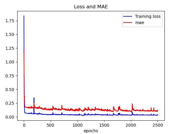
Preprints (www.preprints.org) | NOT PEER-REVIEWED | Posted: 22 March 2021 doi:10.20944/preprints202008.0565.v2

 Peer-reviewed version available at Appl. Sci. 2020, 10, 6819; doi:10.3390/app10196819

 Appl. Sci. 2020, 10, x FOR PEER REVIEW 11 of 13

 (a) (b)
 Figure 9 The mean absolute error and the training loss with GRU before (a) and after (b) standard
 deviation normalization

 4.3.1. Result analysis- Mean Absolute Error (MAE)

 In statistics, the mean absolute error (MAE) is one of the metrics to evaluate how close the
 forecasts are to the eventual outcomes. In the machine learning field, it can indirectly reflect the
 accuracy and performance of the machine learning model (GRU). In this work, we adapted the MAE
 to assess the performance of the GRU for depth estimation with infrared thermography. As we can
 see from Figure 9 (a), we trained the GRU to estimate the data from testing before the data
 normalization. The obtained training loss is 0.055. The MAE converged to 0.0165mm. The error
 between the predictive value and actual value is within the range of [−0.17mm, 0.17mm]. After the
 standard deviation normalization for all the distributed data in Figure 9 (b), the predictive value
 tends to approach the actual depth for the defect. The MAE error shrinks to the range of
 [−0.11mm, 0.11mm] and the training loss converged to 0.0295. This shows an acceptable
 performance with an improved estimate of the depth by the GRU model with standard deviation
 normalization.
 In table 4, the estimated output 1 and the MAE 1 are obtained from raw data without
 normalization (average values over the two estimated outputs from CFRP specimen groups: (A, C);
 (B, D)). Then, the estimated output 2 and the MAE 2 result from raw data of the same procedure but
 with normalization.
 Based on Table 2, the calculated accuracy in the GRU model for the depth estimation reached 90
 % before data normalization (standard deviation). After normalization, the results provide an
 accuracy greater than 95 %. This performance demonstrated that the GRU enable a high performance
 for accurate depth estimation. This estimation is attributed to the ideal environment without
 experimental issues (noise; defective pixels). As shown in the Figure 10 below, the thermal data
 distribution from training (before; after) normalization has been indicated. In the data distribution(a),
 each group of color data curves (yellow; red; green) represents a different specific depth from defects.
 The thermal data is normalized by Eq. (10) in Figure 10 (b). The distinguishable features of difference
 between the depths is recognized by the following principle: shallow defects have greater maximum
 thermal contrasts that occur earlier than deep defects. These results outperformed the previous works

Preprints (www.preprints.org) | NOT PEER-REVIEWED | Posted: 22 March 2021 doi:10.20944/preprints202008.0565.v2

 Peer-reviewed version available at Appl. Sci. 2020, 10, 6819; doi:10.3390/app10196819

 Appl. Sci. 2020, 10, x FOR PEER REVIEW 12 of 13

 obtained from [7] for depth estimation in automated infrared thermography with regular neural
 networks.

 (a) (b)
 Figure 10 The data distribution before (a) and after (b) standard deviation normalization from all the
 selected locations for training

 5 Conclusion

 This work elaborated the complicated and non-linear issues of evaluating defect depths in
 composite materials via infrared thermography with a GRU learning model. The methodology
 proposed here employed a GRU model combined with pulsed thermography to analyze the depth of
 defects. The simulated samples provide an economical platform for GRU training and depth
 estimation. Quantitative analysis of defect depth (subsurface features) has been evaluated by a GRU
 based statistical method through developed neural network modeling and cross validation
 experimental verification. It has been proven that the GRU modeling can produce an advanced depth
 detection. For future work, the experimental data have to be evaluated for the robustness of the GRU
 model. Further, other types of deep learning models and modified versions of the GRU model have
 to be applied to increase the depth estimation ability in this topic.

 Author Contributions: Q.F.; conceived and designed the experiments, Q.F.; proposed the methodology,
 Q.F.; F.A.M performed the experiment, Q.F.; performed the data analyses and wrote manuscript,
 X.M.; reviewed and edited manuscript, X.M.; supervised the project. All authors have read and
 agreed to the published version of the manuscript.

 Funding: This research received funding support from NSERC DG program, the Canada Foundation
 for Innovation and the Canada Research Chair program. We want also to acknowledge the financial
 support and help of the Chinese Scholarship Council.

 Acknowledgments: This research is conducted under the Tier One-Multipolar Infrared Vision Canada
 Research Chair (MIVIM) in the Department of Electrical and Computer Engineering at Laval
 University.

Preprints (www.preprints.org) | NOT PEER-REVIEWED | Posted: 22 March 2021 doi:10.20944/preprints202008.0565.v2

 Peer-reviewed version available at Appl. Sci. 2020, 10, 6819; doi:10.3390/app10196819

 Appl. Sci. 2020, 10, x FOR PEER REVIEW 13 of 13

 Conflicts of Interest: The authors declare no conflict of interest.

 References
 1. D’Accardi E, Palano F, Tamborrino R, et al. Pulsed phase thermography approach for the characterization
 of delaminations in cfrp and comparison to phased array ultrasonic testing[J]. Journal of Nondestructive
 Evaluation, 2019, 38(1): 20.
 2. Nikolas Rajic. Principal component thermography for flaw contrast enhancement and flaw depth
 characterisation in composite structures. Composite Structures, 58(4) :521– 528, 2002
 3. Martin, R.E., Gyekenyesi, A.L., Shepard, S.M.: Interpreting the results of pulsed thermography data. Mater.
 Eval. 61(5), 611–616 (2003)
 4. Shepard, S.M., Lhota, J.R., Rubadeux, B.A., Wang, D., Ahmed, T.: Reconstruction and enhancement of
 active thermographic image sequences. Opt. Eng. 42(5), 1337–1342 (2003)
 5. Weng J, Zhang Y, Hwang W S. Candid covariance-free incremental principal component analysis[J]. IEEE
 Transactions on Pattern Analysis and Machine Intelligence, 2003, 25(8): 1034-1040.
 6. Sun J G. Analysis of pulsed thermography methods for defect depth prediction[J]. 2006.
 7. Darabi A, Maldague X. Neural network-based defect detection and depth estimation in TNDE[J]. Ndt & E
 International, 2002, 35(3): 165-175.
 8. Schlessinger M. Infrared technology fundamentals[M]. Routledge, 2019.
 9. Saeed N, Abdulrahman Y, Amer S, et al. Experimentally validated defect depth estimation using artificial
 neural network in pulsed thermography[J]. Infrared Physics & Technology, 2019, 98: 192-200.
 10. Peeters J, Steenackers G, Ribbens B, et al. Finite element optimization by pulsed thermography with
 adaptive response surfaces[C]//QIRT 2014: the 12th International Conference on Quantitative Infrared
 Thermography, 7-11 July, Bordeaux. 2014.
 11. Lopez F, de Paulo Nicolau V, Ibarra-Castanedo C, et al. Thermal–numerical model and computational
 simulation of pulsed thermography inspection of carbon fiber-reinforced composites[J]. International
 Journal of Thermal Sciences, 2014, 86: 325-340.
 12. Hu C, Duan Y, Liu S, et al. LSTM-RNN-based defect classification in honeycomb structures using infrared
 thermography[J]. Infrared Physics & Technology, 2019, 102: 103032.
 13. Chung J, Gulcehre C, Cho K H, et al. Empirical evaluation of gated recurrent neural networks on sequence
 modeling[J]. arXiv preprint arXiv:1412.3555, 2014.
 14. Gers F A, Schmidhuber J. Recurrent nets that time and count[C]//Proceedings of the IEEE-INNS-ENNS
 International Joint Conference on Neural Networks. IJCNN 2000. Neural Computing: New Challenges and
 Perspectives for the New Millennium. IEEE, 2000, 3: 189-194.
 15. Kassam S. Quantization based on the mean-absolute-error criterion[J]. IEEE Transactions on
 Communications, 1978, 26(2): 267-270.
 16. Horn R A. The hadamard product[C]//Proc. Symp. Appl. Math. 1990, 40: 87-169.
 17. Hochreiter S, Schmidhuber J. Long short-term memory[J]. Neural computation, 1997, 9(8): 1735-1780
 18. Chung J, Gulcehre C, Cho K H, et al. Empirical evaluation of gated recurrent neural networks on sequence
 modeling[J]. arXiv preprint arXiv:1412.3555, 2014.

 © 2020 by the authors. Submitted for possible open access publication under the terms
 and conditions of the Creative Commons Attribution (CC BY) license
 (http://creativecommons.org/licenses/by/4.0/).