A magnetic cloud prediction model for forecasting space weather relevant properties of Earth-directed coronal mass ejections
←
→
Page content transcription
If your browser does not render page correctly, please read the page content below
Astronomy & Astrophysics manuscript no. aanda                                                                                    ©ESO 2022
                                               March 22, 2022

                                                A magnetic cloud prediction model for forecasting space weather
                                                  relevant properties of Earth-directed coronal mass ejections
                                                                                  Sanchita Pal12 , Dibyendu Nandy23 , and Emilia K. J. Kilpua1

                                                     1
                                                         Department of Physics, University of Helsinki, P.O. Box 64, FI-00014 Helsinki, Finland
                                                     2
                                                         Center of Excellence in Space Sciences India, Indian Institute of Science Education and Research Kolkata, Mohanpur 741246,
                                                         West Bengal, India
                                                     3
                                                         Department of Physical Sciences, Indian Institute of Science Education and Research Kolkata, Mohanpur 741246, West Bengal,
                                                         India
                                                         e-mail: sanchita.pal@helsinki.fi
arXiv:2203.05231v2 [astro-ph.SR] 21 Mar 2022

                                                    March 22, 2022

                                                                                                                ABSTRACT

                                                    Context. Coronal Mass Ejections (CMEs) are energetic storms in the Sun that result in the ejection of large-scale magnetic clouds
                                                    (MCs) in interplanetary space that contain enhanced magnetic fields with coherently changing field direction. The severity of CME
                                                    induced geomagnetic perturbations depends on the direction and strength of the interplanetary magnetic field (IMF), as well as the
                                                    speed and duration of passage of the magnetic cloud associated with the storm. The coupling between the heliospheric environment
                                                    and Earth’s magnetosphere is the strongest when the IMF direction is persistently southward for a prolonged period. Predicting
                                                    the magnetic profile of such Earth-directed CMEs is crucial for estimating their geomagnetic impact; this remains an outstanding
                                                    challenge.
                                                    Aims. Our aim is to build upon and integrate diverse techniques towards development of a comprehensive magnetic cloud prediction
                                                    (MCP) model that can forecast the magnetic field vectors, Earth-impact time, speed and duration of passage of solar storms.
                                                    Methods. The configuration of a CME is approximated as a radially expanding force-free cylindrical structure. Combining near-Sun
                                                    geometrical, magnetic and kinematic properties of CMEs with the probabilistic drag based model and cylindrical force-free model we
                                                    propose a methodology for predicting the Earth-arrival time, propagation speed, and magnetic vectors of MCs during their passage
                                                    through 1 AU. A novelty of our scheme is the ability to predict the passage duration of the storm without recourse to computationally
                                                    intensive, time-dependent dynamical equations.
                                                    Results. Our methodology is validated by comparing the MCP model output with observations of ten MCs at 1 AU. In our sample,
                                                    we find that eight MCs show a root mean square (rms) deviation of less than 0.1 between predicted and observed magnetic profiles
                                                    and the passage duration of seven MCs fall within the predicted range.
                                                    Conclusions. Based on the success of this approach, we conclude that predicting the near-Earth properties of MCs based on analysis
                                                    and modelling of near-Sun CME observations is a viable endeavor with potential benefits for space weather assessment.
                                               Use \titlerunning to supply a shorter title and/or \authorrunning to supply a shorter list of authors.
                                               1. Introduction                                                       erties, soon after their origin at the Sun. Depending on the lo-
                                                                                                                     cation of the CME source, CME properties are subject to pro-
                                               Understanding space weather and its variability has become in- jection effect (Burkepile et al. 2004; Howard et al. 2008). Ap-
                                               creasingly important as we rely more and more on the space- plying forward modelling technique (Thernisien et al. 2006) to
                                               borne technology and interconnected power-grids which are sen- white-light CMEs observed simultaneously from different van-
                                               sitive to disturbance from the Sun (e.g., Schrijver et al. 2015). tage points in space, one can reproduce CME’s 3D morphol-
                                               Coronal mass ejections (CMEs; Webb & Howard 2012) are one ogy and estimate deprojected geometrical parameters and kine-
                                               of the most important drivers of severe space weather events. matics (Bosman et al. 2012; Shen et al. 2013). The next step
                                               Their flux rope (FR) structures can be observed in white-light is to evaluate how the initial parameters evolve after the CME
                                               coronagraphs near-Sun (e.g., Vourlidas et al. 2017), and in situ is launched from the Sun. CMEs can experience changes in
                                               observation in interplanetary space (e.g., Kilpua et al. 2017). their space weather relevant properties and propagation direc-
                                               When the twisted magnetic FR of a CME contains southward tion (e.g., Manchester et al. 2017; Kilpua et al. 2019). Firstly,
                                               magnetic field components, magnetic reconnection with the CMEs expand during their interplanetary propagation (Burlaga
                                               Earth’s magnetosphere ensues and leads to effective solar wind et al. 1981; Burlaga 1991). A study by Démoulin & Dasso (2009)
                                               mass, momentum, and energy transfer to the Earth’s magneto- demonstrates that the rapid decrease of solar wind pressure with
                                               sphere. This generates significant ring current enhancement and increasing distance from the Sun is the main driver of the radial
                                               results in a geomagnetic storm (Tsurutani et al. 1988; Gonzalez expansion of CMEs. The deflection of a CME can change sig-
                                               et al. 1999). Therefore, prior knowledge of the magnetic prop- nificantly the latitude and longitude of its propagation direction
                                               erties of Earth-directed CMEs is crucial for reliably predicting (Isavnin et al. 2014; Kay & Opher 2015). In addition, CMEs can
                                               their geoeffectiveness and space weather impacts.                     experience fast and large rotation (e.g., Vourlidas et al. 2011;
                                                    The first step in estimating the geomagnetic response for a Isavnin et al. 2014). These are common phenomena in the solar
                                               given CME is to estimate its initial parameters including their corona due to the presence of strong magnetic forces (Isavnin
                                               structure, propagation direction, kinematics and magnetic prop- et al. 2014; Kay et al. 2015). Deflections and rotations occur
                                                                                                                                                                  Article number, page 1 of 12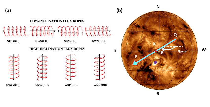
A&A proofs: manuscript no. aanda

also further out in interplanetary space due to the interaction of   tary Flux ROpe Simulator (INFROS) developed by Sarkar et al.
a CME with the background solar wind magnetic fields (Wang           (2020) includes the flux rope expansion in a way to get rid of
et al. 2004) and preceding or following CMEs (Wang et al. 2004,      expansion and propagation speed and time of passage. It deter-
2014). Deflections can cause CMEs that were initially not head-      mines the time varying axial field intensity and derives axial field
ing towards the Earth to impact us or re-route Earth-directed        direction and FR chirality using EUV, H-alpha and magnetogram
CMEs away from our planet (e.g., Möstl et al. 2015). The rota-       observations of their sources. This approach allows constrain-
tion in turn changes the magnetic field profile finally impacting    ing the FR parameters in a more realistic manner for event to
the Earth, and thus influences the geoeffectivity (Palmerio et al.   event basis (see also Palmerio et al. 2017; Kilpua et al. 2019; Pal
2018). Interaction of a CME FR with the ambient open flux may        2021). The models discussed above however do not incorporate
also result in flux erosion impacting geoeffectiveness (Pal et al.   CME arrival time prediction and unable to predict the flux rope
2020). All of these phenomena is a challenge for the prediction      passage time.
of near-Earth CME properties, which nonetheless, is highly de-           In this paper we present a comprehensive empirical mod-
sirable.                                                             elling framework that builds upon our knowledge to predict var-
     The distortion of CME’s geometrical structure can be ob-        ious space weather relevant characteristics of a CME magnetic
served in coronagraphs. However, the influence of distortion on      cloud near Earth. The model, which we name the CESSI-MCP
CME’s magnetic structure is hard to estimate because the mag-        model does not involve FR dimension, FR axial field intensity,
netic field cannot yet be reliably measured in the hot and tenu-     FR arrival time and speed as free parameters. It has some unique
ous corona. To estimate CME’s magnetic vectors few studies use       characteristics, a particular novelty being that it utilizes CME’s
solar observations as input to three-dimensional magnetohydro-       arrival time and speed along with considerations of self-similar
dynamic (MHD) models of CME evolution (Manchester et al.             expansion to predict the passage duration of the CME FR. In
2004; Shen et al. 2014). Although data driven physical MHD           Section 2 we describe the model and outline procedures for es-
models for CME flux rope strucure prediction are desirable from      timating the model inputs. In Section 3 we validate our model
the intellectual perspective, such models are computationally ex-    using in situ observed MC events. The results are critically as-
pensive (Manchester et al. 2014) and does not have enough ob-        sessed in Section 4 and we conclude with a summary discussion
servations in the inner heliosphere to constrain their evolution.    in Section 5.
     Various alternative semi-empirical modelling approaches
have been proposed for prediction of the magnetic structure
of CMEs. Using analytical and semi-analytical models which           2. Methodology: Modeling MCs
approximate CMEs as force-free cylindrical flux-ropes, several       2.1. MCP model description
studies have performed predictions of the magnetic structure of
CME flux ropes as they arrive near the Earth’s orbit (Savani         To examine the configuration of MCs we assume them to be
et al. 2015; Kay & Gopalswamy 2017; Möstl et al. 2018; Sarkar        force free (Goldstein 1983), i.e., J = αB, where J and B repre-
et al. 2020). One key aspect of these models is to constrain the     sent the current density and magnetic field vector, respectively.
magnetic properties of the CME flux rope as it leaves the Sun.       Marubashi (1986) used first the model allowing α to vary with
The model by Savani et al. (2015) uses as default the “Bothmer-      the distance from the MC centre to fit two MCs. Later, Burlaga
Schwenn” scheme (Bothmer & Schwenn 1998). This scheme re-            (1988) showed that α can be considered as constant to describe
lies on hemispheric helicity rule (Pevtsov & Balasubramaniam         a magnetic cloud in the first order. For constant α the solutions
2003), which states that the northern (southern) hemisphere is       of the force-free model in cylindrical co-ordinates are obtained
dominated by magnetic structures with negative (positive) he-        by Lundquist (1951), where the axial (Bax ), azimuthal (Baz ), and
licity sign and assumes that the orientation of the flux rope’s      radial (Brad ) magnetic field components are given by,
axial field follows the polarity of the leading and trailing flux
                                                                     Bax = B0 J0 (αρ),                                               (1)
systems in active regions. The hemispheric rule applies only in
a statistical sense and intrinsic AR magnetic properties such as
tilt orientation and twist themselves have a large scatter (Nandy
2006). Models of coronal field evolution and CME genesis based       Baz = HB0 J1 (αρ),                                              (2)
on active regions properties often miss out a large proportion of
events (Yeates et al. 2010) implying a gap in our understanding.     and
A study by Liu et al. (2014) showed that in only 60% of the          Bρ = 0,                                                         (3)
case the hemispheric helicity rule is followed in predicting the
CME’s flux rope chirality. In addition, rising CME flux ropes in-    respectively. In Equation 2 H represents the chirality of cylin-
teract with overlying coronal fields and this interaction is cycle   drical FRs. The right and left-handed chirality of FRs are indi-
phase dependent (Cook et al. 2009). This may alter the amount        cated by H = 1 and H = −1, respectively. The axial magnetic
of magnetic flux and helicity as they reconnect with the overly-     field intensity of FRs is represented by B0 . The zeroth and first
ing coronal arcades during the CME lift-off. These further com-      order Bessel functions of first kind are shown by J0 and J1 , re-
pound the problem of predictions.                                    spectively. The parameter ρ is the radial distance from MC axis,
     Some approaches have been proposed recently to make head-       and α is related to FR size. The value of α is chosen so that
way in the face of these challenges. The ForeCAT (Forecasting a      αR MC = 2.41, where 2.41 is the first zero of J0 and R MC is the
CME’s Altered Trajectory) In situ Data Observer (FIDO) model         radius of MC.
developed by Kay & Gopalswamy (2017) and the 3-Dimensional               The field configuration described in Equation 1 and 2 is
Coronal ROpe Ejection (3DCORE) model developed by Möstl              static. Burlaga et al. (1981); Burlaga (1991) indicated the ex-
et al. (2018) take into account the expanding nature of the CME’s    panding nature of MCs causing smooth decrease in solar wind
FR as it crosses the observing spacecraft in interplanetary space    speed and low solar wind proton temperature during their in-
and use extreme ultraviolet (EUV) observations to identify FR        tervals. Démoulin et al. (2008); Démoulin & Dasso (2009) per-
foot point direction and chirality. The formulation of Interplane-   formed theoretical studies on the expansion of MCs. The studies
Article number, page 2 of 12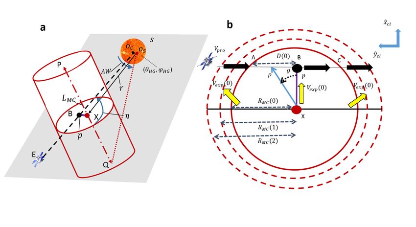
Sanchita Pal et al.: A magnetic cloud prediction model for forecasting space weather relevant properties of Earth-directed coronal mass ejections

concluded that MCs expand self-similarly resulting in a linear                    et al. 2003; Schwenn et al. 2005; Gopalswamy et al. 2012). As
radial velocity profile of MCs and the rate of MC expansion is                    mentioned in the Introduction, the reason of CME’s expansion is
proportional to the MC radius. The expansion of MC was first                      mainly the decaying solar wind pressure surrounding the CME.
modeled by Osherovich et al. (1993) later followed by other                       The expansion is rapid within a distance ≈ 0.4 AU from the Sun
studies, including, Marubashi (1997); Hidalgo (2003); Vandas                      and becomes moderate at large distance (Scolini et al. 2021).
et al. (2006), and Marubashi & Lepping (2007). These models                       Lepping et al. (2008) formulated the ‘scalar derivation’ of expan-
are intended to fit the velocity magnitude profile of MCs. It is                  sion speed of FRs near the Earth that uses FR width, propagation
assumed that in an asymptotic limit, an FR expands radially with                  speed, and duration of FR passage. As the formulation depends
a speed                                                                           on the unknown free parameters like FR duration, we utilise the
                                                                                  value of FR average expansion speed at 1 AU estimated by pre-
            ρ
Vexp =           ,                                                        (4)     vious statistical studies. Lepping et al. (2008) analysed 53 MCs
          t + t0                                                                  of standard profiles and obtained their expansion speed using
where the force free field configuration is maintained at any in-                 two different methods namely the “scalar” method and “vector
stant of time t (Shimazu & Vandas 2002; Vandas et al. 2006,                       determination”. They found the most probable values of expan-
2015). In a self-similar expansion, the t0 in Equation 4 repre-                   sion speed to be around 30 km/s. Nieves-Chinchilla et al. (2018)
sents the time by which the expansion of FR has proceeded be-                     studied a large number (337) of ICMEs observed by Wind space-
fore it comes into contact with the spacecraft. If a self-similarly               craft during 1995 - 2015 and reported that MC expansion speed
expanding MC changes its radius from its initial value R MC (0) to                ranges from - 56 to 271 km/s with the mean value of 28 km/s.
                                                                                                                         t=0
R MC (t) by the time t, the R MC (t) can be represented as R MC (t) =             Therefore, we consider the value of Vexp    as 28 km/s in our study.
R MC (0)(1 + tt0 ). Thus, for an expanding FR, α and B0 become                        To obtain the model parameters specifically p, R MC0 , B00 and
                                                α0                    B00         H the near-Sun observations of the associated CME FRs are uti-
time-dependent and are expressed as α =       (1+ tt )
                                                         and B0 =   (1+ tt )2
                                                                              ,   lized. As discussed in the Introduction, the significant deflection
                                                   0                     0
where α0 = 2.41/R MC (0) and B00 is the axial magnetic field inten-               and rotation of CMEs regularly occur near the Sun, within 10R
sity when the MC first encounters with the spacecraft. Consid-                    (Kay & Opher 2015; Lynch et al. 2009). We assume here that the
ering the expansion of the MC along radial and axial directions                   propagation direction, axis orientation, and chirality of CMEs
Equation 1 & 2 are modified as                                                    obtained at a height > 10R remain unchanged throughout their
                                                                                  Sun-Earth propagation. The radius and magnetic field intensity
         B00 J0 ( (1+α0t ) ρ)                                                     of CMEs are in turn assumed to evolve from their values approx-
                      t0
Bax =                           ,                                         (5)     imated at ∼ 10R due to self-similar expansion (Subramanian
            (1 + tt0 )2                                                           et al. 2014; Vršnak et al. 2019) in the course of interplanetary
                                                                                  propagation. In the following sections we discuss the procedures
                                                                                  used in determination of model parameters.
           B00 J1 ( (1+α0t ) ρ)
                           t0
Baz = H                             ,                                     (6)
               (1 +    t 2
                      t0 )                                                        2.2. Estimates of the geometrical properties of FRs

where the force free condition is assumed to be preserved                         We estimate CME’s three-dimensional morphology and propa-
throughout the propagation of MCs.                                                gation direction in the outer corona ∼ 10 − −25R by fitting the
     Knowledge of the perpendicular distance (p) between an                       geometrical structure of CMEs using graduated cylindrical shell
MC axis and the location of a spacecraft performing the in                        (GCS) model (Thernisien 2011). The CMEs are observed in C2
situ measurements of the MC is necessary to obtain ρ. Fig-                        & C3 coronagraphs of Large Angle and Spectrometric Corona-
ure 2 shows a cylindrical MC and its expanding cross-section.                     graph (LASCO) telescope on board the Solar and Heliospheric
The MC expands with a velocity Vexp and its axis propagates                       Observatory (SOHO) and COR2 A & B of Sun Earth Connec-
with a speed V pro . In the FR frame of reference it is assumed                   tion Coronal and Heliospheric Investigation (SECCHI) on board
that the spacecraft propagates with the speed V pro . At the in-                  the Solar Terrestrial Relations Observatory (STEREO). By fit-
bound and out-bound regions of the MC the Vexp is added to                        ting the CMEs with GCS model, we obtain the latitude (θHG ) and
and subtracted from the ambient solar wind speed, respectively,                   longitude (φHG ) of the apex of CMEs in Stonyhurst heliographic
to obtain V pro (Vandas et al. 2015). For 0 < p < R MC the                        coordinates, the tilt η (−90◦ < η < 90◦ ) of the axis of FR CMEs,
                                                   q                              aspect ratio (κ), height (hl ) of the CME leading edges and the
ρ(t) = p2 + (D2 (t) − V pro (t) × t), where D(t) = R2MC (t) − p2 .
         p
                                                                                  angle (AW) formed between the two legs of CME FRs. The FR
Thus at t = 0, when an MC first encounters the spacecraft,                        axis tilt η is measured as counterclockwise positive from the so-
ρ(0) = R MC (0). Figure 2 is shown in the FR frame of refer-                      lar West direction. The uncertainty in determining η using GCS
ence where the spacecraft traverses through the MC with a speed                   is ±10◦ (Thernisien et al. 2009). Sarkar et al. (2020) considered
V pro . The schematic shown in Figure 2(a) represents the cross-                  uncertainties of ±10◦ in θHG & φHG determinations and ±10% in
ing of a spacecraft through an MC via a path ‘AC’ indicated by                    obtaining κ. Using θHG , φHG , and ηcme we formulate the FR axis
black dash line. The MC axis is shown by a blue dashed line                       and considering the Earth’s location as (θHG , φHG ) = (0, 0) we
and the circumference of the MC cross-section is indicated by a                   define p as
red dashed circle. The centre of the MC is pointed by ‘O’, and
                                                                                       |θHG − φHG tan(η)|
‘OB’ represents the distance p. In Figure 2(b) the expanding MC                   p=                      .                                       (7)
                                                                                            1 + tan2 (η)
                                                                                          p
cross-section is shown. At t = 0, the circle made of solid red line
represents the MC cross-section circumference where the dis-
                                                                                  Using κ that constrains the FR expansion, R MC (0) can be deter-
tance ‘AB’ is equivalent to D(0). Once we obtain the value of
                                                                                  mined by
Vexp at t = 0, we can estimate t0 value from t0 = Vexp
                                                    t=0
                                                        /R MC (0).
     Several studies have related radial speed (Vrad ) and expan-                              height MC
sion speed (Vexp ) of CME’s FRs at the near-Sun region (Dal Lago                  R MC (0) =             ,                                        (8)
                                                                                                1 + 1/κ
                                                                                                                          Article number, page 3 of 12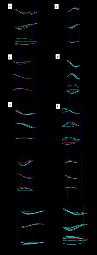
A&A proofs: manuscript no. aanda
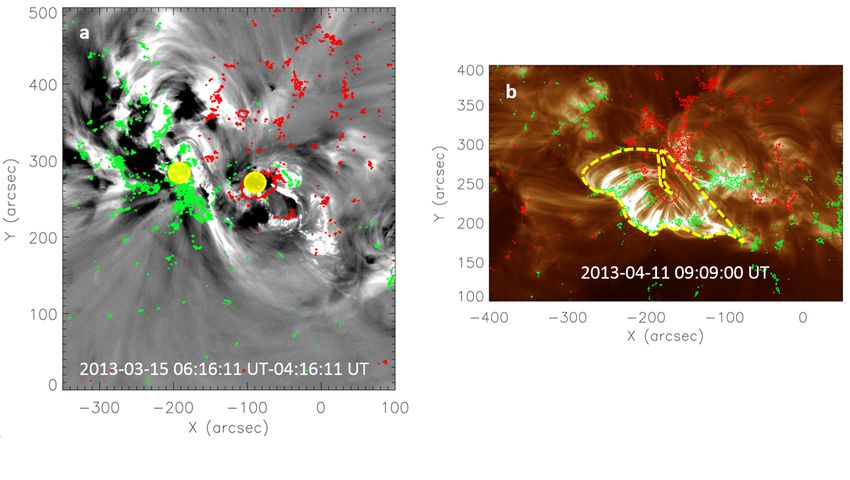
where height MC is the leading-edge height of MCs reaching at for EUV dimming signatures in SDO/AIA 211 Å base-difference
the Earth. Thus, it is equivalent to the Sun-Earth distance. The images and overlie LOS magnetogram data on them. Thus, we
length (L MC ) of the FR axis at any heliocentric distance (r) is obtain the magnetic polarities of FR foot points. The FR axial
obtained using AW by the formula L MC = (AW ×r), where AW is field is directed from positive to negative foot points. In Figure
in radian. In Figure 3(a), we show a schematic of cylindrical FR 4(a) we indicate FR foot points by yellow circles on the EUV dif-
with the Sun, Earth and spacecraft positions. The CME source ference image obtained using observations from SDO/AIA 211
location (‘s’), apex (‘X’), tilt, angular width (AW), heliocentric Å. The LOS magnetogram with LOS magnetic field intensity
distance (r), L MC and p are indicated on the Figure. The centre of BLOS > ±150 G is over-plotted on the EUV difference image us-
the Sun and Earth are denoted by ’c‘ and ‘E‘, respectively. Figure ing red (negative magnetic field region) and green (positive mag-
3(b) shows a South-East directed MC FR axis ‘PQ’ projected on netic field region) contours. After obtaining chirality, FR axis tilt
the solar disk with a positive η measured anti-clockwise from the and axial field direction we infer the flux rope type.
East-West direction. The Earth’s location (θHG , φHG ) = (0, 0))
projected on the solar disk is noted by ‘E’.
2.3.3. Measuring the axial magnetic field intensity ( B00 ) of
FRs
2.3. Estimation of flux-rope’s near-Sun magnetic properties
To estimate the axial magnetic field strength BCME of CMEs near
The magnetic field pattern of a flux rope can be expressed in the Sun, we apply the “flux rope from eruption data” (Gopal-
terms of a “flux rope (FR) type" (Bothmer & Schwenn 1998; swamy et al. 2017, FRED) technique that requires source-region
Mulligan et al. 1998). The FR type can be determined using FR reconnection flux Frec , i.e., the photospheric magnetic flux under
chirality – right-handed or left-handed twist of the FR’s helical CME associated post-eruption arcades and the length (LCME ) &
magnetic field component, FR axis tilt, and the direction of FR radius (RCME ) of CMEs. The reconnection flux is obtained us-
axial magnetic field. Based on these properties, FRs are classi- ing the method discussed in Gopalswamy et al. (2017a); Gopal-
fied into eight different types including low and high-inclination swamy et al. (2017b). It is equivalent to the poloidal or azimuthal
FR axes. A sketch representing eight types of FRs are shown in flux (F pcme ) of CME FRs (Longcope et al. 2007; Qiu et al. 2007).
Figure 3(a). The poloidal flux of CMEs is conserved during their interplane-
tary propagation (Qiu et al. 2007; Hu et al. 2014; Gopalswamy
et al. 2017a; Pal 2021) unless CME flux is significantly eroded
2.3.1. Determination of FR chirality due to reconnection in heliosphere. Thus, B00 is estimated using,
To estimate the handedness of FRs we analyse the Helioseismic RCME
Magnetic Imagers (HMI) line-of-sight (LOS) magnetograms, B00 = BCME × . (9)
R MC (0)
Atmospheric Imaging Assembly (AIA) images on board Solar
Dynamic Observatory (SDO) and H-α images of the FRs’ so- In Figure 4(b) a PEA region is indicated by yellow dashed
lar sources. The chirality of the solar source indicates the chi- line on SDO/AIA 193 Å image where the positive and negative
rality of the associated FR in the corona and further out in in- magnetic field regions are shown by green and red contours, re-
terplanetary space as magnetic helicity is a conserved quantity spectively.
even in magnetic reconnection (Berger 2005). The chirality is
inferred by examining magnetic tongues (Fuentes et al. 2000;
2.4. Estimation of the arrival time and transit speed of CMEs
Luoni et al. 2011), dextral and sinistral natures of filament struc-
tures (Martin & McAllister 1996; Martin 2003), EUV sigmoids, Along with magnetic profile, we estimate the CME arrival time a
skew of coronal arcades overlying the neutral lines or filament 1AU and transit speed utilizing a pre-existing probabilistic drag-
axes (McAllister et al. 1995; Martin & McAllister 1997), struc- based ensemble model (DBEMv3; Čalogović et al. 2021; Dum-
ture of flare-ribbons associated with CME FRs (Démoulin et al. bović et al. 2018) – an upgraded version of a simple kinematic
1996) and hemispheric helicity rule (Bothmer & Schwenn 1998). drag based model (DBM; Vršnak et al. 2013) established us-
These chirality proxies are briefly discussed in Palmerio et al. ing the concept of aerodynamic drag on interplanetary propa-
(2017). Note that, the hemispheric helicity rule (see the Intro- gation of CMEs. The model DBEMv3 produces possible dis-
duction) can be utilised to estimate CME FRs’ chirality as first tributions of CME arrival information by employing ensemble
order approximation if CME associated solar sources are unam- modeling of CME propagation. It assumes CME to be a cone
biguously determined. structure with semicircle leading edge spanning over its angular
width where the structure flattens with the CME’s interplane-
2.3.2. Determination of flux rope type of CMEs tary evolution (Žic et al. 2015). It considers solar wind speed
(V sw ) and drag parameter (γ) to be constant beyond the dis-
The orientation of the flux-rope axis roughly follows the as- tance of 15 R . This is because beyond 15 R CMEs propa-
sociated PIL (Marubashi et al. 2015) or post-eruption arcades gate through an isotropic solar wind having a constant velocity.
(PEAs; Yurchyshyn 2008) orientations. The flux ropes however Also, the rate of the fall-off of solar wind density is similar to the
often undergo significant rotations in the lower corona during the rate of the self-similar expansion of CMEs (Vršnak et al. 2013;
early evolution due to interactions with overlying skewed coro- Žic et al. 2015). The DBEMv3 is available at Hvar Observatory
nal loops (Lynch et al. 2009). To take into account the possi- website as an online tool (http://phyk039240.uni-graz.
ble rotation in the corona we determine FR’s axis orientation (η) at:8080/DBEMv3/dbem.php) which is a product of European
from GCS at the height greater than 10 R from the Sun and Space Agency (ESA) space situational awareness (SSA). The in-
use that in our prediction tool. We obtain the FR foot points on put to the model are CME initial speed VCME with uncertainty
solar surface using EUV images and magnetograms. The foot ±∆VCME , half angular width λ projected on the plane-of-sky
points are determined by coronal dimming regions formed dur- with uncertainty ±∆λ, propagation longitude φHG with uncer-
ing the flux-rope rise period (Mandrini et al. 2005). We search tainty ±∆φHG at a specific radial distance R0 , CME arrival time
Article number, page 4 of 12Sanchita Pal et al.: A magnetic cloud prediction model for forecasting space weather relevant properties of Earth-directed coronal mass ejections
tlaunch at R0 with uncertainty ±∆tlaunch along with the radial speed 3. Results: Model validation using observed MC
of solar wind V sw ± ∆V sw and drag parameter γ ± ∆γ. We pre- events
pare an ensemble of n measurements of a single CME, and m
number of V sw & γ using their uncertainty ranges. Thus, a to- As a proof of concept we validate our model by investigating
tal number of n.m2 input sets are prepared for analysis. After ten Earth-directed MCs appearing as FRs at near-Sun and in
performing n.m2 number of runs the DBEMv3 produces distri- situ regions, and having clearly identified solar sources. At the
butions of n.m2 number of arrival times and speeds. Here we near-Earth region (L1 Lagrangian point) MCs are observed us-
assume that at 1 AU, the plasma propagation speed (V pro ) within ing Magnetic Field Experiment (MAG) instrument of the Ad-
CMEs is almost equal to its average Sun-Earth transition speed vanced Composition Explorer (ACE) spacecraft. The events are
Vtr (Lepping et al. 2008). To prepare the inputs to DBEMv3 we selected from the Richardson & Cane ICME catalog (Richardson
utilise CME parameters obtained from GCS fitting results where & Cane 2010, ; http://www.srl.caltech.edu/ACE/ASC/
the GCS model has been fitted to CMEs at a height more than DATA/level3/icmetable2.html). The front and rear bound-
10 R . We derive CME initial speed VCME and its arrival time at aries of the MCs are verified manually such that at 1 AU they
R0 = 21.5R by least-square fitting its height-time profile. Fol- maintain the MC properties suggested by Burlaga et al. (1981)
lowing Čalogović et al. (2021), the uncertainties ∆tlaunch , ∆λ, and throughout their interval and their associated CMEs appear as
∆φHG are set to ±30 min, ±10% and ±5◦ , respectively. For each isolated magnetic structures in near-Sun observations.
CME, the drag parameter γ is selected based on their speed. The
values of γ are empirical-based, (Vršnak et al. 2013, 2014; Žic 3.1. Preparation of model inputs
et al. 2015). For CMEs with VCME < 600 km/s, the γ is set to
0.5×10⁻⁷ ±0.1 km−1 , for 600 km/s < VCME < 1000 km/s, the γ is We manually identify each of the MC associated CMEs follow-
set to 0.2×10⁻⁷ ±0.075 km−1 and for VCME > 1000 km/s the γ is ing Zhang et al. (2007); Pal et al. (2017) and locate their solar
set to 0.1 × 10⁻⁷ ± 0.05 km−1 (Čalogović et al. 2021). To estimate sources utilizing their coronal signatures observed in SDO/AIA.
the ambient solar wind speed (V sw ) we follow the Empirical solar We obtain CME’s geometrical parameters θHG , φHG , AW, η, and
wind forecast (ESWF; Vršnak & Žic 2007; Vršnak et al. 2007; κ at a height hl > 10R and tabulate them in Column 5-10 of
Rotter et al. 2012, 2015; Reiss et al. 2016) processes that moni- Table 1, respectively. The GCS fitting to FRs associated with
tor fractional areas covered by coronal holes close to the central Event 4 and 7 CMEs can be found in Figure 5 and 1 of Pal et al.
meridian region. We follow an algorithm based on an empirical (2017) and Pal et al. (2018), respectively. We define CME ini-
relation that links the area of coronal holes appeared close to the tiation time (CME start ) as the moment when the CMEs are first
central meridian (±10◦ ) and solar wind speed. The empirical re- identified at SOHO/LASCO C2 field of view. In Column 1 and 2
lationship follows the equation V sw (t) = c0 + c1 A(t − δt), where the event numbers (Ev no.) and CME start are mentioned, respec-
A is the fractional coronal hole area. We shift coronal hole area tively. Column 3 and 4 contain the start (MC start ) and end time
time series with a time lag δt to determine the V sw at time t. Vrš- (MCend ) of MCs adapted from the Richardson & Cane ICME
nak et al. (2007) studied this empirical relationship during the catalog.
period DOY 25 – 125 of the year 2005 and found δt = 4 days, Utilizing V sw (derived using empirical relationship between
c0 = 350 km/s and c1 = 900. They found that the average relative coronal hole area and solar wind speed), drag parameter, CME’s
difference between the predicted and observed peak solar wind deprojected velocity, longitude and projected angular width and
speed valuesis ±10%. Therefore, we consider ∆V sw = ±10% their uncertainties as input, DBEMv3 estimates the probability
(ptar ) of CME arrival at Earth, arrival time and arrival speed dis-
tributions. The median tar of arrival time distribution with 95%
confidence intervals (tar,LCI < tar < tar,HCI ) are mentioned in
Column 5 of Table 2. We compute CME transit speed Vtr using
2.5. Coordinate conversion of magnetic field vectors Sun-Earth distance and tar . The error in arrival time prediction
is obtained from terr = tar − MC start . We present Vtr and terr in
Column 6 and 7. In Column 2, 3, and 4 of Table 2, we provide
At 1 AU, the inclination angle (θ MC ) of MCs is considered to extrapolated deprojected speed of CMEs at 21.5 R , V sw during
be equivalent to the η of associated CMEs and the azimuthal an- CME propagation, and ptar , respectively. We obtain the mean
gle (φ MC ) of MCs are determined using CME propagation lon- absolute error (MAE) in prediction of CME arrival time as ∼6.3
gitudes (φHG ) obtained at 10 R . In order to express Baz , Bax hours.
and Bρ in Geocentric Solar Ecliptic (GSE) coordinate system (a To determine FR types, we obtain their chirality, axis orien-
Cartesian coordinate system where ẑ is perpendicular to the Sun- tations, and axial magnetic field directions using remote obser-
Earth plane, and x̂ is parallel to the Sun-Earth line and positive vations as described before. The multi-wavelength proxies men-
toward the Sun) that is majorly used to represent the magnetic tioned in Section 2.3.1 are examined for all MCs to infer their
field vectors of ICMEs at 1 AU, we transform the field vectors chirality. We convert PEA tilt and FR axis tilt η into the orien-
from local cylindrical to Cartesian coordinate system. At first tation angles ηarcade and ηcme respectively, which lie within the
Baz , Bax , and Bρ are converted to Bx,cl , By,cl and Bz,cl which are in range [−180◦ , 180◦ ]. The angles are measured from the solar
local Cartesian coordinate ( x̂cl , ŷcl , ẑcl ) system originating at MC west direction, counterclockwise for positive and clockwise for
axis. Finally, using θ MC & φ MC , the magnetic field vectors Bx,cl , negative values. They are derived by taking into account the ax-
By,cl and Bz,cl are transformed to Bx , By and Bz . ial field direction that is estimated using coronal dimming in-
formation. Yurchyshyn (2008) studied the relation between PEA
angles and CME directions of 25 FR events and found that for
In Figure 1, we present our MC prediction approach using a majority of events the difference between the angles remains less
block-diagram where yellow coloured blocks represent the mod- than 45◦ . In Table 3, we summarise the near-Sun FR magnetic
els and techniques used in our approach and sky-blue coloured properties of ten events. Column 1 shows the Event numbers,
blocks indicate the model parameters and outputs. Column 2 shows flux-rope chirality, where ‘+1’ stands for right-
Article number, page 5 of 12A&A proofs: manuscript no. aanda
Table 1. Near-Sun observations of CME latitude (θHG ), longitude (φHG ), tilt (η), aspect ratio (κ), height (hl ) of the CME leading edges and the
angular width (AW), their initiation time (CME start ), and associated MCs’ start (MC start ) and end times (MCend ).
Ev CME start MC start MCend Durobs θHG φHG η (◦ ) AW κ hl
no. (UT) (UT) (UT) (hr) (◦ ) (◦ ) (◦ ) (R )
(1) (2) (3) (4) (5) (6) (7) (8) (9) (10) (11)
1 2010/05/24 2010/05/28 2010/05/29 20 0 5.3 −53.3 36 0.22 11.4
14:06:00 20:46:00 16:27:00
2 2011/06/02 2011/06/05 2011/06/05 17 −7.8 −11.8 55.3 34 0.15 14.7
08:12:00 01:50:00 19:00:00
3 2012/02/10 2012/02/14 2012/02/16 33 28 −23 −72 50 0.23 13.5
20:00:00 20:24:00 05:34:00
4 2012/06/14 2012/06/16 2012/06/17 16 0 −5 30.7 76 0.30 15
14:12:00 22:00:00 14:00:00
5 2012/07/12 2012/07/15 2012/07/17 47 −8 14 53.1 60 0.66 14.1
16:48:00 06:00:00 05:00:00
6 2012/11/09 2012/11/13 2012/11/14 24 2.8 −4 −2 36 0.20 12.4
15:12:00 09:44:00 02:49:00
7 2013/03/15 2013/03/17 2013/03/18 11 −6.5 −10 −74.4 51 0.27 18
07:12:00 14:00:00 00:45:00
8 2013/04/11 2013/04/14 2013/04/15 28 −5.5 −15 68.2 74 0.24 20.5
07:24:00 16:41:00 20:49:00
9 2013/06/02 2013/06/06 2013/06/08 33 −1.7 7 75.5 36 0.21 12.14
20:00:00 14:23:00 00:00:00
10 2013/07/09 2013/07/13 2013/07/15 43 2 3 −37.5 36 0.36 13.4
15:12:00 04:39:00 00:00:00
Table 2. A table containing CME speed (VCME ), solar wind speed (VS W ), probability of CME arrival at Earth (ptar ), predicted arrival time range
(tar,LCI < tar < tar,HCI ), predicted Sun-Earth transition speed (Vtr ) and the difference terr between the observed and predicted arrival time median
values.
Ev VCME VS W ptar tar,LCI < tar < tar,HCI Vtr terr
no.
km/s km/s % UT km/s Hr
(1) (2) (3) (4) (5) (6) (7)
1 562±60 350±35 100 228-05-2010 05:57 < 28-05-2010 10:05 < 28-05-2010 14:42 450 −10.7
2 937±20 356±36 100 04-06-2011 20:09 < 05-06-2011 00:11 < 05-06-2011 04:17 646 −1.7
3 658±13 352±35 51 14-02-2012 05:05 < 14-02-2012 09:41 < 14-02-2012 13:35 482 −10.7
4 1020±60 350±35 100 16-06-2012 13:57 < 16-06-2012 17:31 < 16-06-2012 21:00 806 −4.5
5 1000±200 363±36 100 15-07-2012 00:20 < 15-07-2012 05:42 < 15-07-2012 11:15 679 −0.3
6 611±24 350±35 100 12-11-2012 18:22 < 12-11-2012 21:22 < 13-11-2012 00:38 529 −11
7 1160±28 355±35 100 17-03-2013 02:47 < 17-03-2013 06:20 < 17-03-2013 09:59 877 −7.7
8 700±24 371±37 99.8 14-04-2013 07:55 < 14-04-2013 11:53 < 14-04-2013 16:40 599 −4.8
9 500±70 350±35 100 06-06-2013 16:42 < 06-06-2013 22:17 < 07-06-2013 04:47 383 7.9
10 610±30 350±35 100 12-07-2013 21:28 < 13-07-2013 00:37 < 13-07-2013 04:04 508 −4
handedness and ‘−1’ represents left-handedness. In Column 3, 4 sociated MCs intersecting the spacecraft at 1 AU. To incorporate
and 5 we present ηarcade , ηcme and their difference ηdi f f , where the ambiguities involved in measurements of propagation direc-
positive value of ηdi f f represents rotation of CME axis in coun- tion, inclination, and size of CMEs we utilize the uncertainty
terclockwise with respect to PEA tilt. range of those parameters as input to our model. We prepare ten
As ηcme is measured at a coronal height (≥ 10 R ) greater different random input sets of each MC where the input param-
than that where the ηarcade is measured, we utilise ηcme as the eter values are within ±10◦ of measured propagation direction
final value of FR axial orientation. Combining ηcme , chirality, and and ηcme , and ±10% of estimated κ value. The magnetic field
FR axis direction, we estimate the type of CME FRs, typens and vectors are derived using each of the input sets. Thus, we obtain
mention it in Column 6 of Table 3. Finally, the axial magnetic ten different magnetic profiles for every event and measure the
field intensity of the associated CMEs are derived using F pcme root-mean-square (rms) differences between observed and pre-
and FR geometrical parameters. Column 7 of Table 3 shows the dicted magnetic vectors. The normalised rms difference (∆rms )
F pcme of near-Sun FRs. is calculated using the ratio of δB and Bomax , where Bomax is the
maximum observed magnetic field intensity and δB is defined
by,
3.2. Model outputs
Using the near-Sun CME observations as input to the constant- rP
o − Bp (ti ))2
α force-free cylindrical FR model that expands self-similarly in i (B (ti )
δB = . (10)
radial directions we estimate the magnetic field vectors of the as- N
Article number, page 6 of 12Sanchita Pal et al.: A magnetic cloud prediction model for forecasting space weather relevant properties of Earth-directed coronal mass ejections
Table 3. CME’s near-Sun magnetic properties – PEA tilt (ηarcade ), CME axis orientation (ηcme ), their differences (ηdi f f ), near-Sun FR type (typens )
and axial magnetic field intensity (F pcme ).
Ev no. Chirality ηarcade ηcme ηdi f f typens F pcme
(◦ ) (◦ ) (◦ ) (1021 Mx)
(1) (2) (3) (4) (5) (6) (7)
1 LH −19.3 −53.3 −34 WSE 2.15
2 RH 46.2 55.3 9 WNE 1.81
3 RH 110.2 72 −38.2 ESW 2
4 RH −127.4 −149.3 −22 NES 8.45
5 RH −151 −127 24 ESW 14.10
6 RH −172 178 −6 NES 2.47
7 RH 123 105.6 −17.4 ESW 4.10
8 LH −61.5 −111.8 −50.3 ENW 3.72
9 LH 137.7 75.5 −62.2 WSE 1.75
10 LH −39.2 −37.5 1.7 NWS 3.50
MC , θ MC ) and longitude (φ MC , φ MC ) of MC axes derived from observed and predicted magnetic field vectors, predicted
Table 4. Latitude (θmva m mva m
normalised impact parameters (Y0m ), differences in observed and predicted magnetic field vectors (∆rms ), near-Earth observed FR types (typene ),
comparison of near-Sun and near-Earth FR types Cor and minimum and maximum values of predicted duration ranges (Dur pred,min − Dur pred,max ).
Ev no. θmva
MC φmva ◦
MC ( ) θmMC (◦ ) φmMC (◦ ) Y0m ∆m
rms typene Cor Dur pred,min -Dur pred,max
(◦ ) ◦
() (◦ ) (◦ ) (Hr)
(1) (2) (3) (4) (5) (6) (7) (9) (10) (11)
1 −69 244.5 −60 273 0.5 0.07 WSE y 27 - 41
(LH)
2 45.8 193 59 281 −0.62 0.22 WNE y 14 - 20
(RH)
3 −10.5 271 -64 307 -0.2 0.1 ESW y 33 - 43
(RH)
4 −7.5 102.4 −30.6 84.1 −0.15 0.08 NES y 19 - 22
(RH)
5 −76.3 183.9 −62.7 151 0.73 0.07 ESW y 38 - 50
(RH)
6 8 83.4 3.3 84.7 −0.1 0.07 NES y 16 - 33
(RH)
7 −15.9 16 −72 297.5 0.72 0.2 SWN n 20 - 25
(RH)
8 59.8 337 74.7 304 −0.54 0.1 ENW y 10 - 24
(LH)
9 −81.7 193.2 −70.9 97.24 0.28 0.06 WSE y 28 - 57
(LH)
10 −9 284 −36 263.7 −0.53 0.05 NWS y 35 - 57
(LH)
Here Bo (ti ) and Bp (ti ) are the observed and predicted mag- by θmMC , φmMC and Y0m , respectively. We apply minimum variance
netic field vectors, respectively, and i = 1, 2, 3...N with N be- analysis (Sonnerup & Cahill 1967) to the in situ measurements
ing the total number of data points in predicted magnetic vec- and estimate the orientation (latitude θmvaMC , and longitude φ MC )
mva
tors. The observed magnetic field vector is binned with a bin of MCs at 1 AU, in order to compare the predicted and observed
size=( MCend −MC
N
start
). We obtain MC axis orientations (θmMC , φmMC ) orientations. In Column 2 and 3 of Table 4, we present θmva MC and
and impact parameters corresponding to those predicted MC φmva
MC values. We mention the values of θ m
MC , φm
MC , Y0
m
, and ∆m
rms
magnetic profiles having minimum value of ∆rms . The ∆rms of ten MCs in Column 4, 5, 6, and 7 of Table 4, respectively.
is estimated for Bx , By and Bz , separately and represented by The magnetic type of the MCs (typene ) as observed by ACE are
∆rms
x
, ∆yrms and ∆zrms , respectively. In Figure 5 we display the pre- noted in Column 9. To compare the magnetic field orientation
dicted magnetic vectors obtained from the model along with the in predicted and observed FRs at 1 AU, we utilise the parameter
in situ data measured at L1 by ACE/MAG instrument for ten Cor in Column 8. Here ‘y’ and ‘n’ indicate a match and mismatch
MCs. The observed solar wind magnetic field vectors are shown in field line orientation of near-Sun and near-Earth FRs, respec-
in black whereas the red curves over plotted on them during MC tively. The event numbers (Ev no.) are mentioned in Column 1.
intervals (indicated by dashed blue vertical lines) represent the Using R MC and plasma propagation speed inside FRs, we esti-
predicted fields having minimum value of ∆rms . The uncertain- mate a range of predicted duration values (Dur pred ) for each FR
ties in predictions resulted from errors in input estimations are at 1 AU. We mention the minimum (Dur pred,min ) and maximum
shown using cyan dotted curves. The latitude, longitude, nor- (Dur pred,max ) values of Dur pred range in Column 11 of Table 4.
malised impact parameter Y0m = RMCp (0) corresponding to the min- The observed MC duration Durobs values are mentioned in Col-
imum value of ∆rms , i.e., ∆m umn 5 of Table 1. By comparing the minimum and maximum
rms of individual cases are denoted
Article number, page 7 of 12A&A proofs: manuscript no. aanda
values of Dur pred and Durobs , it can be noticed that the Durobs of netic field asymmetry and a large asymmetry is marked with
Event 1, 4 and 7 does not fall in Dur pred range and is less than |C B | > 0.1 (Lanabere et al. 2020). We obtain C B = −0.12 in
Dur pred,min by 8, 3 and 10 hours, respectively. We notice that the case of Event 2, which is greater than |C¯B | ± δ|C B | = 0.04 ± 0.04
over-estimation in Dur pred is mostly caused due to error in Vtr derived for other events. Here |C¯B | and δ|C B | indicate the mean
and FR radius estimations. and standard deviation of C B values, respectively. It implies that
a circular-cross section model is inappropriate to estimate its
magnetic profile. In Figure 6(a) we show the in situ asymmet-
4. Discussion ric magnetic field intensity B of Event 2 MC. The interval within
the vertical lines represents MC interval. The FR associated with
The modelling framework presented here allows prior estimates Event 7 rotates significantly while propagating from the Sun to
of the magnetic field profile of MCs at 1 AU, their arrival time, Earth and results in a comparatively high value of ∆m rms . Due to
average speed while crossing the Earth and duration of passage rotation, the FR type changes from the near-Sun to near-Earth re-
thus providing comprehensive intelligence on impending space gions for this event. By comparing the θmvaMC and θ MC of this event,
m
weather events. we find that the FR changes its type from high-inclination (the
The approach constrains CME FRs using remote solar central axis is more or less perpendicular to the ecliptic plane)
observations and takes into account the radial expansion of to low-inclination (the central axis is more or less parallel to the
MCs. It assumes MCs to expand self-similarly during their ecliptic plane) while propagating in the interplanetary medium.
Sun-Earth propagation. The geometric and kinematic parame- Based on statistical evidence, Yurchyshyn (2008); Yurchyshyn
ters of MCs are constrained using GCS fitting to the white- et al. (2009) and Isavnin et al. (2013) suggested that MCs rotate
light coronagraph images of associated CMEs at a height towards the heliospheric current sheet (HCS; Smith 2001) so that
greater than 10 R , while their magnetic parameters are con- they stay aligned with the local HCS. We consider the Wilcox so-
strained using remote observations of their solar sources. Once lar observatory coronal field map calculated from synoptic pho-
the near-Sun CME parametrization is performed, our ana- tospheric magnetogram with a potential field model (Hoeksema
lytical model takes only a few seconds to predict the pro- et al. 1983; Hoeksema 1984) during Carrington rotation (CR)
files and estimates the approximate duration of Earth-directed 2134 when the eruption associated with Event 7 occurred. Utilis-
CMEs. The near-real time data (≈ 6 hour before the cur- ing θHG and φHG we infer the CME locations on the coronal field
rent time) from LASCO and SECCHI coronagraphs are avail- map. We observe that in order to stay aligned with the HCS the
able in https://sohoftp.nascom.nasa.gov/qkl/lasco/ associated CME axis underwent significant rotation (≈ 56◦ ) and
quicklook/level_05 and https://stereo-ssc.nascom. became more or less parallel to the ecliptic plane by the time it
nasa.gov/data/beacon/, respectively. Also, the near-real reached at 2.5 R . For context, in Figure 6(b) we show a coronal
time observations (≈ 1 hour before the current time) of solar map during CR 2134 obtained from http://wso.stanford.
atmosphere and photospheric magnetic field from AIA and HMI edu/synsourcel.html. The grey solid contours represent the
on board SDO spacecraft are available in https://sdowww. positive field region, whereas the dotted contours indicate the
lmsal.com/suntoday_v2/ and https://jsoc.stanford. negative field region. The black thick solid line represents the lo-
edu/data/hmi/fits/, respectively. Using these resources, the cation of HCS. The pink circle indicates the CME location and
model is able to predict the properties of CMEs reaching the dotted and solid pink lines show the before and after-rotation
Earth within 6 hours of their initiation from the Sun. Typically, CME axis orientation, respectively.
CMEs may take 15 hours to several days to reach Earth after Sarkar et al. (2020) noted that the Bx component is more
leaving the Sun. To predict the arrival of FRs at Earth the drag- sensitive to small variations (±10◦ ) in the CME’s propagation
based ensemble model is applied. direction and tilt than the By and Bz components. They found
We apply the CESSI-MCP modelling framework to predict that within the propagation direction uncertainties, the Bx com-
the magnetic profile of ten Earth-directed CMEs having clear in ponent of MCs may have both positive and negative components.
situ signatures at 1 AU and remote observations of solar sources. In our study we observe that the uncertainty in CME’s direction
We derive the r.m.s error between observed and predicted pro- of propagation and tilt leads to a significant variation in predicted
files to estimate the quality of prediction. The values of r.m.s Bx profiles of MCs associated with Event 1, 3, 4, 6 and 10 (see
error (see Column 7 of Table 4) suggest that for most of the the blue dotted lines in the third panel of Figure 5(a), (c), (d), (f)
cases, the predicted magnetic field magnitude and vector time se- and (j) have both positive and negative values).
ries show a good agreement with in situ observations. We notice For obtaining deprojected geometrical parameters and kine-
that ∆mrms for Event 2 and 7 is greater than 2× (average (∆rms ) ±
¯m
matics of CMEs, simultaneous observations from different van-
standard deviation (σ∆rms )) of ∆rms values associated with other
m
m
tage points in space are necessary (Bosman et al. 2012). Bosman
events. Although Event 2 has similar FR type at near-Sun and (2016) demonstrated that to resolve a CME well globally (3-D)
near-Earth region (typens = typene = WNE), there exists a sig- from 2-D plane-of-sky images obtained using coronagraphs on
nificant asymmetry in its magnetic field strength between in- board spacecrafts, the angular separation ζ between the space-
bound (while spacecraft propagates towards MC centre) and out- crafts need to be large, i.e., 10◦ < ζ ≤ 90◦ . If ζ is in between
bound (while spacecraft propagates away from MC centre) paths 0◦ − 10◦ , the 2-D plane-of-sky images obtained from two coro-
which might enhance the value of ∆m rms . The asymmetry does not nagraphs on board two separate spacecrafts become nearly con-
occur only because of FR expansion or ageing effect (Démoulin gruent, whereas a value of ζ = 90◦ , provides the best condi-
et al. 2008, 2018). Rather, most of the MC field strength asym- tion to resolve a CME in 3-D. (Thernisien et al. 2009). The out-
metry is due to non-circular cross section of FRs (Démoulin & of-ecliptic observations of Metis: multi-wavelength coronagraph
Dasso 2009). Janvier et al. (2019); Lanabere et al. (2020) quanti- for the Solar Orbiter mission and potential L5 and L4 solar mis-
RMC start t−tc
B(t)dt sions are expected to have significant contributions in enhancing
fied the FR asymmetry C B as C B =
MCend MCend −MC start
R MC start , where
MCend
B(t)dt the precision of CME parameterisation.
B(t) is the magnetic field strength and tc = (MC start + MCend )/2 The presented framework to estimate the magnetic field time
represents the central time. Therefore, |C B | increases with mag- evolution of the near-Earth crossing of MCs, their arrival time
Article number, page 8 of 12Sanchita Pal et al.: A magnetic cloud prediction model for forecasting space weather relevant properties of Earth-directed coronal mass ejections
and passage duration appears very promising. As discussed in Dumbović, M., Čalogović, J., Vršnak, B., et al. 2018, The Astrophysical Journal,
the Introduction the capability to estimate reliably the time series 854, 180
Fuentes, M. L., Démoulin, P., Mandrini, C. H., & van Driel-Gesztelyi, L. 2000,
of Bz is crucial for space weather forecasting. The Astrophysical Journal, 544, 540
However, this approach is not expected to perform well in Goldstein, H. 1983, in NASA Conference Publication, Vol. 228, NASA Confer-
some cases, e.g., the case of strongly interacting CMEs, e.g., ence Publication
where CMEs interact significantly with other CMEs and extra- Gonzalez, W. D., Tsurutani, B. T., & De Gonzalez, A. L. C. 1999, Space Science
neous magnetic transients, when their propagation is influenced Reviews, 88, 529
Gopalswamy, N., Akiyama, S., Yashiro, S., & Xie, H. 2017, Proceedings of the
by fast stream originating from nearby coronal holes, when their International Astronomical Union, 13, 258
configuration is influenced by the heliospheric current sheet Gopalswamy, N., Akiyama, S., Yashiro, S., & Xie, H. 2017b, Journal of Atmo-
and fast solar wind stream, or when their cross-sections differ spheric and Solar-Terrestrial Physics
strongly from a circular shape. Gopalswamy, N., Makela, P., Yashiro, S., & Davila, J. M. 2012, Sun and Geo-
sphere, 7, 7
Gopalswamy, N., Yashiro, S., Akiyama, S., & Xie, H. 2017a, Solar Physics, 292,
65
5. Conclusions Hidalgo, M. 2003, Journal of Geophysical Research (Space Physics), 108
Hoeksema, J. T. 1984, Structure and Evoluton of the Large Scale Solar and He-
In this paper, we develop a scheme to predict the time series of liospheric Magnetic Fields., Tech. rep., STANFORD UNIV CA CENTER
magnetic field vectors of CME associated magnetic clouds dur- FOR SPACE SCIENCE AND ASTROPHYSICS
ing their near-Earth passage, estimate their arrival time, speed Hoeksema, J. T., Wilcox, J. M., & Scherrer, P. H. 1983, Journal of Geophysical
and duration of passage. The CESSI-MCP model is completely Research: Space Physics, 88, 9910
Howard, T., Nandy, D., & Koepke, A. 2008, Journal of Geophysical Research
constrained by solar disk/near-Sun observations, is fast, has a (Space Physics), 113
large time window for predictions and can be easily transitioned Hu, Q., Qiu, J., Dasgupta, B., Khare, A., & Webb, G. M. 2014, The Astrophysical
in to operational forecasting. The ability to perform all these Journal, 793, 53
tasks at high fidelity, including predicting the passage duration Isavnin, A., Vourlidas, A., & Kilpua, E. K. J. 2013, Sol. Phys., 284, 203
Isavnin, A., Vourlidas, A., & Kilpua, E. K. J. 2014, Sol. Phys., 289, 2141
of MCs are significant from the space weather perspective. Janvier, M., Winslow, R. M., Good, S., et al. 2019, Journal of Geophysical Re-
We believe the enhanced functional utility of our methodol- search: Space Physics, 124, 812
ogy is due to a combination of factors, including, constraining Kay, C. & Gopalswamy, N. 2017, Journal of Geophysical Research (Space
the CME flux rope realistically using solar observations and al- Physics), 122, 11
lowing the expansion of its cross-section. Our work emphasizes Kay, C. & Opher, M. 2015, The Astrophysical Journal Letters, 811, L36
Kay, C., Opher, M., & Evans, R. M. 2015, ApJ, 805, 168
the importance of near-Sun observations, multi-vantage points Kilpua, E., Koskinen, H. E. J., & Pulkkinen, T. I. 2017, Living Reviews in Solar
observations, and in situ observations in deriving realistic intrin- Physics, 14, 5
sic parameters of CMEs from the Sun to near-Earth. Kilpua, E. K. J., Lugaz, N., Mays, M. L., & Temmer, M. 2019, Space Weather,
17, 498
Acknowledgements. The development of the CESSI magnetic cloud prediction Lanabere, V., Dasso, S., Démoulin, P., et al. 2020, Astronomy & Astrophysics,
(CESSI-MCP) model was performed at the Center of Excellence in Space Sci- 635, A85
ences India (CESSI) at the Indian Institute of Science Education and Research, Lepping, R. P., Wu, C. C., Berdichevsky, D. B., & Ferguson, T. 2008, Annales
Kolkata. S.P. and E.K. acknowledge support from the European Research Coun- Geophysicae, 26, 1919
cil (ERC) under the European Union’s Horizon 2020 Research and Innovation Liu, Y., Hoeksema, J., Bobra, M., et al. 2014, The Astrophysical Journal, 785,
Program Project SolMAG 724391 and the frame work for the Finnish Centre 13
of Excellence in Research of Sustainable Space (FORESAIL; Academy of Fin- Longcope, D., Beveridge, C., Qiu, J., et al. 2007, Solar Physics, 244, 45
land grant numbers 312390). The authors acknowledge the use of data from the Lundquist, S. 1951, Phys. Rev., 83, 307
STEREO, SDO, SOHO and ACE instruments. The PhD research of S.P. was Luoni, M. L., Démoulin, P., Mandrini, C. H., & van Driel-Gesztelyi, L. 2011,
supported by the Ministry of Education, Government of India. Solar Physics, 270, 45
Lynch, B., Antiochos, S., Li, Y., Luhmann, J., & DeVore, C. 2009, The Astro-
physical Journal, 697, 1918
Manchester, W., Kilpua, E. K. J., Liu, Y. D., et al. 2017, Space Science Reviews,
References 212, 1159
Manchester, W. B., Gombosi, T. I., Roussev, I., et al. 2004, Journal of Geophys-
Berger, M. A. 2005, Highlights of Astronomy, 13, 85 ical Research (Space Physics), 109, A02107
Bosman, E. 2016, PhD thesis, Georg-August-Universität Göttingen Manchester, W. B., van der Holst, B., & Lavraud, B. 2014, Plasma Physics and
Bosman, E., Bothmer, V., Nisticò, G., et al. 2012, Solar Physics, 281, 167 Controlled Fusion, 56, 064006
Bosman, E., Bothmer, V., Nisticò, G., et al. 2012, Solar Physics, 281, 167 Mandrini, C. H., Pohjolainen, S., Dasso, S., et al. 2005, Astronomy & Astro-
Bothmer, V. & Schwenn, R. 1998, Annales Geophysicae, 16, 1 physics, 434, 725
Burkepile, J. T., Hundhausen, A. J., Stanger, A. L., St.Cyr, O. C., & Seiden, J. A. Martin, S. & McAllister, A. 1996, in Magnetodynamic phenomena in the solar
2004, Journal of Geophysical Research (Space Physics), 109 atmosphere (Springer), 497–498
Burlaga, L. 1988, Journal of Geophysical Research (Space Physics), 93, 7217 Martin, S. & McAllister, A. 1997, Washington DC American Geophysical Union
Burlaga, L. 1991, Journal of Geophysical Research (Space Physics), 96, 5847 Geophysical Monograph Series, 99, 127
Burlaga, L., Sittler, E., Mariani, F., & Schwenn, R. 1981, Journal of Geophysical Martin, S. F. 2003, Advances in Space Research, 32, 1883
Research (Space Physics), 86, 6673 Marubashi, K. 1986, Advances in Space Research, 6, 335
Burlaga, L., Sittler, E., Mariani, F., & Schwenn, R. 1981, Journal of Geophysical Marubashi, K. 1997, Coronal mass ejections, 99, 147
Research (Space Physics), 86, 6673 Marubashi, K., Akiyama, S., Yashiro, S., et al. 2015, Solar Physics, 290, 1371
Čalogović, J., Dumbović, M., Sudar, D., et al. 2021, Solar Physics, 296, 1 Marubashi, K. & Lepping, R. P. 2007, Annales Geophysicae, 25, 2453
Cook, G., Mackay, D., & Nandy, D. 2009, Astrophys. J., 704, 1021 McAllister, A., Hundhausen, A., Burkpile, J., McIntosh, P., & Hiei, E. 1995, in
Dal Lago, A., Schwenn, R., & Gonzalez, W. D. 2003, Advances in Space Re- Bulletin of the American Astronomical Society, Vol. 27, 961
search, 32, 2637 Möstl, C., Amerstorfer, T., Palmerio, E., et al. 2018, Space Weather, 16, 216
Démoulin, P. & Dasso, S. 2009, Astronomy & Astrophysics, 498, 551 Möstl, C., Rollett, T., Frahm, R. A., et al. 2015, Nature Communications, 6, 7135
Démoulin, P. & Dasso, S. 2009, A&A, 507, 969 Mulligan, T., Russell, C., & Luhmann, J. 1998, Geophysical Research Letters,
Démoulin, P., Dasso, S., & Janvier, M. 2018, A&A, 619, A139 25, 2959
Démoulin, P., Nakwacki, M. S., Dasso, S., & Mandrini, C. H. 2008, Solar Nandy, D. 2006, Journal of Geophysical Research: Space Physics, 111
Physics, 250, 347 Nieves-Chinchilla, T., Vourlidas, A., Raymond, J., et al. 2018, Solar Physics,
Démoulin, P., Nakwacki, M. S., Dasso, S., & Mandrini, C. H. 2008, Sol. Phys., 293, 1
250, 347 Osherovich, V., Farrugia, C., & Burlaga, L. 1993, Journal of Geophysical Re-
Démoulin, P., Priest, E., & Lonie, D. 1996, Journal of Geophysical Research search (Space Physics), 98, 13225
(Space Physics), 101, 7631 Pal, S. 2021, Advances in Space Research
Article number, page 9 of 12You can also read