PROJECTED LATENT MARKOV CHAIN MONTE CARLO: CONDITIONAL SAMPLING OF NORMALIZING FLOWS
←
→
Page content transcription
If your browser does not render page correctly, please read the page content below
Published as a conference paper at ICLR 2021

P ROJECTED L ATENT M ARKOV C HAIN M ONTE C ARLO :
C ONDITIONAL S AMPLING OF N ORMALIZING F LOWS
 Chris Cannella, Mohammadreza Soltani & Vahid Tarokh
 Department of Electrical and Computer Engineering
 Duke University

                                           A BSTRACT

         We introduce Projected Latent Markov Chain Monte Carlo (PL-MCMC), a tech-
         nique for sampling from the exact conditional distributions learned by normaliz-
         ing flows. As a conditional sampling method, PL-MCMC enables Monte Carlo
         Expectation Maximization (MC-EM) training of normalizing flows from incom-
         plete data. Through experimental tests applying normalizing flows to missing data
         tasks for a variety of data sets, we demonstrate the efficacy of PL-MCMC for con-
         ditional sampling from normalizing flows.

1   I NTRODUCTION

Conditional sampling from modeled joint probability distributions offers a statistical framework for
approaching tasks involving missing and incomplete data. Deep generative models have demon-
strated an exceptional capability for approximating the distributions governing complex data. Brief
analysis illustrates a fundamental guarantee for generative models: the inaccuracy (i.e. divergence
from ground truth) of a generative model’s approximated joint distribution upper bounds the ex-
pected inaccuracies of the conditional distributions known by the model, as shown in Appendix A.
Although this guarantee holds for all generative models, specialized variants are typically used to
approach tasks involving the conditional distributions among modeled variables, due to the diffi-
culty in accessing the conditional distributions known by unspecialized generative models. Quite
often, otherwise well trained generative models possess a capability for conditional inference that is
regrettably locked away from our access.
Normalizing flow architectures like RealNVP (Dinh et al., 2014) and GLOW (Kingma & Dhariwal,
2018) have demonstrated accurate and expressive generative performance, showing great promise
for application to missing data tasks. Additionally, by enabling the calculation of exact likelihoods,
normalizing flows offer convenient mathematical properties for approaching exact conditional sam-
pling. We are therefore motivated to develop techniques for sampling from the exact conditional
distributions known by normalizing flows. In this paper, we propose Projected Latent Markov Chain
Monte Carlo (PL-MCMC), a conditional sampling technique that takes advantage of the convenient
mathematical structure of normalizing flows by defining a Markov Chain within a flow’s latent space
and accepting proposed transitions based on the likelihood of the resulting imputation. In principle,
PL-MCMC enables exact conditional sampling without requiring specialized architecture, training
history, or external inference machinery.

Our Contributions: We prove that a Metropolis-Hastings implementation of our proposed PL-
MCMC technique is asymptotically guaranteed to sample from the exact conditional distributions
known by any normalizing flow satisfying very mild positivity and smoothness requirements. We
then describe how to use PL-MCMC to perform Monte Carlo Expectation Maximization (MC-EM)
training of normalizing flows from incomplete training data. To illustrate and demonstrate aspects
of the technique, we perform a series of experiments utilizing PL-MCMC to complete CIFAR-10
images, CelebA images, and MNIST digits affected by missing data. Finally, we perform a series of
experiments training non-specialized normalizing flows to model MNIST digits and continuous UCI
datasets from incomplete training data to verify the performance of the proposed method. Through
these experimental results, we find that PL-MCMC holds great practical promise for tasks requiring
conditional sampling from normalizing flows.

                                                  1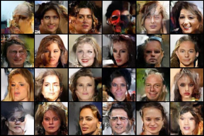
Published as a conference paper at ICLR 2021

2     R ELATED W ORK

A conditional variant of normalizing flows has been introduced by Lu & Huang (2020) to model
a single conditional distribution between architecturally fixed sets of conditioned and conditioning
variables. While quite capable of learning individual conditional distributions, conditional variants
do not enable arbitrary conditional sampling from a joint model. Richardson et al. (2020) concur-
rently train a deterministic inference network alongside a normalizing flow for inferring missing
data. Although such an inference network can produce deterministic imputations consistent with
the distributions learned by a normalizing flow, it cannot stochastically sample from the conditional
distributions known by the flow. Li et al. (2019) introduce shared parameter approximations that
allow the derivation of approximate conditional normalizing flows, though these approximations do
not guarantee exact sampling from the conditional distributions of a particular joint model. Similar
techniques for approaching missing data with other generative models, such as generative adver-
sarial networks (GANs) and variational auto-encoders (VAEs), have been introduced with similar
limitations (Ivanov et al., 2018; Yoon et al., 2018; Li et al., 2018).
A MCMC procedure for sampling from the conditional distributions of VAEs has been introduced
by Rezende et al. (2014) and refined by Mattei & Frellsen (2018). This procedure fundamentally
relies on the many-to-many relationship between the latent and modeled data spaces of VAEs, and
cannot be directly applied to normalizing flows, wherein the latent state uniquely determines (and
is uniquely determined by) the modeled data state. By following an unconstrained Markov Chain
within the latent space, PL-MCMC mirrors this VAE conditional sampling procedure within the
context of normalizing flows.
PL-MCMC leverages the probabilistic structure learned by a normalizing flow to produce efficient
Markov Chains. The utility of the mathematical structure of normalizing flows for approaching
Monte Carlo estimation via independence sampling has been demonstrated by Müller et al. (2019).
The probabilistic structure of normalizing flows has also been shown to improve unconditional sam-
pling from externally defined distributions by Hoffman et al. (2019). In using this learned structure,
we believe that PL-MCMC receives many of the benefits of Adaptive Monte Carlo methods (Haario
et al., 2001; Foreman-Mackey et al., 2013; Zhu, 2019), as explained in Appendix B.
PL-MCMC’s unconstrained Markov Chain through the latent space is not the only conceivable op-
tion for sampling from the conditional distributions described by normalizing flows. As normalizing
flows enable exact joint likelihood calculations, we could employ MCMC methods through the mod-
eled data space. Dinh et al. (2014) demonstrate a stochastic conditional MAP inference that can be
adapted to implement the unadjusted Langevin algorithm (Fredrickson et al., 2006; Durmus et al.,
2019) or the Metropolis adjusted Langevin algorithm (Grenander & Miller, 1994). A constrained
Hamiltonian Monte Carlo approach has also been introduced in the context of conditional sampling
from generative models by Graham et al. (2017). MCMC methods restricted to the modeled data
space approach the normalizing flow as a sort of blackbox oracle to be used only for calculations
regarding data likelihood. By design, PL-MCMC leverages the flow’s one-to-one mapping between
latent and modeled data spaces, thereby taking better advantage of the probabilistic structure learned
by our normalizing flows to perform conditional sampling.

3     T HE PL-MCMC A PPROACH

We consider a normalizing flow between latent space Ξ and modeled data space X , defining the
mappings fθ : Ξ 7→ X and fθ−1 : X 7→ Ξ. This normalizing flow imposes the probability density
pf,θ (x) onto all modeled data values x ∈ X . By the pairing (xM ; xO ), we denote the missing
and observed portion of a modeled data value with joint density pf,θ (xM ; xO ) under our normal-
izing flow. Our goal is to sample from the conditional density described by the normalizing flow,
pf,θ (xM |xO ).

3.1   T HE P ROJECTED L ATENT TARGET D ISTRIBUTION

Rather than targeting the conditional distribution of missing values directly, PL-MCMC targets a
distribution of latent variables that, after mapping through the flow’s transformation, marginalizes
to the desired conditional distribution. Let the Markov Chain be composed of latent state ξ ∈ Ξ,

                                                  2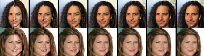
Published as a conference paper at ICLR 2021

mapping to the modeled data pair fθ (ξ) = (yM ; yO ). Let q be an arbitrary smooth density over
observed variables, yO . PL-MCMC targets the distribution whose (unnormalized) density within
the modeled data space is q(yO )pf,θ (yM |xO ). Fundamentally, PL-MCMC is a marginal MCMC
method (Van Dyk, 2010) that uses the otherwise observed attributes, yO , as auxiliary working vari-
ables to take full advantage of the probabilistic structure learned by the normalizing flow.

3.2   D ESCRIPTION OF M ETROPOLIS -H ASTINGS PL-MCMC A LGORITHM

For a Metropolis-Hastings implementation of PL-MCMC, we introduce a transition kernel g(ξ 0 |ξ)
for generating proposal latent states. We sample a new proposal latent vector ξ 0 ∼ g(ξ 0 |ξ), mapping
to the modeled data pair fθ (ξ 0 ) = (y0 M ; y0 O ). An illustrative diagram of the production of PL-
MCMC proposals is provided in Appendix B. This proposal is then accepted with probability:

                                           q(y0 O )pf,θ (y0 M ; xO )g(ξ|ξ 0 )| det ∂f
                                                                                   ∂ξ0 |
                                                                                     θ

                          α = min(1,                                                       ).
                                            q(yO )pf,θ (yM ; xO )g(ξ 0 |ξ)| det ∂f
                                                                                ∂ξ |
                                                                                   θ

Algorithm 1: PL-MCMC Metropolis-Hastings Update
Input: Observed data xO , normalizing flow fθ , modeled joint density pf,θ (xM ; xO ). Latent
         transition kernel g(ξ 0 |ξ) and auxiliary density q(yO ). Initial latent state ξ
Sample ξ 0 ∼ g(ξ 0 |ξ);
yM ; yO ← fθ (ξ);
y0 M ; y0 O ← fθ (ξ 0 );
                                                 ∂fθ
              q(y0 O )pf,θ (y0 M ;xO )g(ξ|ξ0 )| det
                                                 ∂ξ0
                                                     |
α ← min(1,                            0         ∂fθ      );
               q(yO )pf,θ (yM ;xO )g(ξ |ξ)| det ∂ξ |
Sample u ∼ Uniform[0, 1];
if u < α then
     ξ ← ξ0 ;

3.3   T HEORETICAL J USTIFICATION OF THE A LGORITHM

Proposition. For a given xO , if g(ξ 0 |ξ), pf,θ (yM ; yO ), and q(yO ) are positive for any choice of
(yM ; yO ) ∈ X and ξ 0 , ξ ∈ Ξ and are the densities for absolutely continuous distributions, the
PL-MCMC update procedure listed in Algorithm 1 yields a Markov Chain of latent states ξ whose
corresponding modeled data pairs, fθ (ξ) = (yM ; yO ) , converge to a distribution with yM having
marginal density pf,θ (yM |xO ).

Proof. Under these assumptions, the diffeomorphism (i.e, an invertible and differentiable mapping)
provided by the flow fθ allows us to interpret the latent transition kernel g(ξ 0 |ξ) as the transition
                                      ∂f −1
kernel g(fθ−1 (y0 )|fθ−1 (y))| det ∂yθ 0 | within the modeled data space that is positive for all y, y0 ∈
X and is the density for an absolutely continuous distribution. Additionally, we note:

                              q(y0 O )pf,θ (y0 M ; xO )   q(y0 O )pf,θ (y0 M |xO )
                                                        =                          .
                               q(yO )pf,θ (yM ; xO )       q(yO )pf,θ (yM |xO )

The diffeomorphism provided by the flow fθ also guarantees that q(yO )pf,θ (yM |xO ) is positive
for all (yM ; yO ) ∈ X and is the density for an absolutely continuous distribution. The procedure
listed in Algorithm 1 therefore describes a Metropolis-Hastings update satisfying the conditions
described by Tsvetkov et al. (2013). The paired values fθ (ξ) = (yM ; yO ) obtained through iter-
ated application of Algorithm 1 thus converge to a target distribution with (unnormalized) density
q(yO )pf,θ (yM |xO ).

The requirements for convergence are very mild and are satisfied by the most common choices
for latent, transition proposal, and auxiliary distributions (e.g. multivariate normal distributions).
We note that the eventual convergence of the PL-MCMC update towards the desired conditional

                                                              3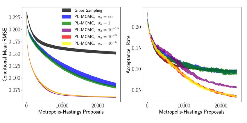
Published as a conference paper at ICLR 2021

distribution is not influenced by our choice of the auxiliary distribution q. However, the choice of
this auxiliary distribution can affect the rate of convergence. We have found agreeable performance
by selecting q to be an independent normal distribution centered on the conditioning values xO .
This guides the Markov Chain towards reasonable samples more quickly by leveraging learned
dependencies between the observed and missing components of the modeled data.

4     T RAINING N ORMALIZING F LOWS FROM M ISSING DATA
With PL-MCMC providing samples from the conditional distributions of normalizing flows, a natu-
ral application of the technique is in MC-EM training (Dempster et al., 1977; Wei & Tanner, 1990;
Neath et al., 2013) of normalizing flows from incomplete data. MC-EM training involves imputing
missing values within the training set via conditional sampling of our current model, and then up-
dating the parameters of our model to best fit the newly imputed training set. As described within
Appendix C, this leads to Algorithm 2, with PL-MCMC(xO,i ; pf,θ , qi ) denoting the distribution ob-
tained by following an implementation of PL-MCMC with auxiliary density qi (defined in 3.1) and
train being any training procedure that returns flow parameters θ approximately maximizing the
likelihood of a complete data training set. For our experimental tests, PL-MCMC is obtained through
iterated application of Algorithm 1.

Algorithm 2: Monte Carlo Expectation Maximization Training of Normalizing Flow
Input: Incomplete training data Xtrain = {xO,1 , xO,2 , . . . , xO,T }. Auxiliary densities qi .
        Normalizing flow training procedure train. Parameterized flow architecture fθ .
while training do
    for i ← 1 to T do
         Sample yM,i ∼ PL-MCMC(xO,i ; pf,θ , qi );
    end
      0
    Xtrain  = {(yM,1 ; xO,1 ), (yM,2 ; xO,2 ), . . . , (yM,T ; xO,T )};
                       0
    θ ← train(f, Xtrain     );
end

Intuitively, this procedure relies on conditional inference to “boost” the accuracy of our current
                                                                                              0
model for the joint distribution governing the training data. At each step of Algorithm 2, Xtrain
represents samples from an approximation of the modeled data’s ground truth distribution. We fit θ
to model this approximate joint distribution. After conditional inference with the new normalizing
                                                0
flow using PL-MCMC, the next iteration of Xtrain      represents samples from a distribution with a
smaller divergence from the ground truth distribution, as discussed in Appendix A. Importantly, this
MC-EM training procedure assumes that data is missing at random (Little & Rubin, 2019).

5     Q UALITATIVE E XPERIMENTAL R ESULTS
For a qualitative examination of the performance of PL-MCMC, we focus on conditionally sampling
missing data using normalizing flows that have been trained from complete data. We must note that
the the purpose of PL-MCMC is to sample from a model’s conditional distributions, which may
not coincide with accurately replicating the ground truth values of missing data. These qualitative
experiments are therefore intended to illustrate aspects of the operation of PL-MCMC and to provide
a visual verification of the method’s performance. Further details of these experiments and examples
of unconditioned samples from the normalizing flows are provided in Appendix D.

5.1   C ONDITIONAL I NFERENCE WITH CIFAR-10 I MAGES

We first consider sampling a missing central quarter of CIFAR-10 (Krizhevsky et al., 2009) images
(32 × 32 full color images) using a normalizing flow following the GLOW architecture (Kingma &
Dhariwal, 2018). To bolster our claim that PL-MCMC does not require specially trained models,
we utilize a publicly available pre-trained model (van Amersfoort, 2019) for this experiment. Initial
and final completions provided by the Markov Chain are illustrated in Figure 1.

                                                    4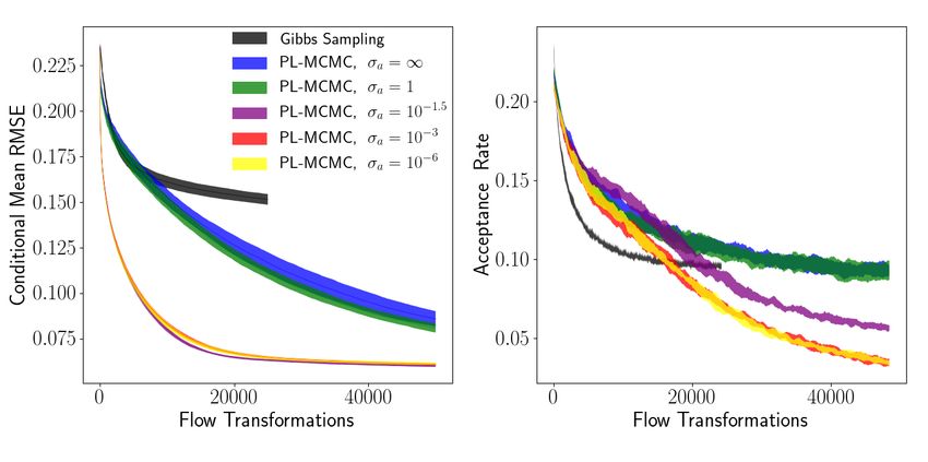
Published as a conference paper at ICLR 2021
(a) Initial Completions (b) Final Completions (c) Ground Truth
Figure 1: Conditional inference of CIFAR-10 images with normalizing flow trained on complete
data.
The initial state of the Markov Chain is constructed by filling pixels with RGB values randomly
selected from the observed subset. Latent space transitions are generated via small perturbations
within the absolute coordinates of the latent space. PL-MCMC is carried out for 25,000 proposals.
Example progressions of completions are provided in Figure 2. In comparison with unconditioned
samples, the PL-MCMC completions appear reasonable, given the capabilities of the underlying
model, and highlight the perceptual benefit provided by conditioned sampling.
Figure 2: Progression of CIFAR-10 completions over intervals of 3,000 PL-MCMC proposals.
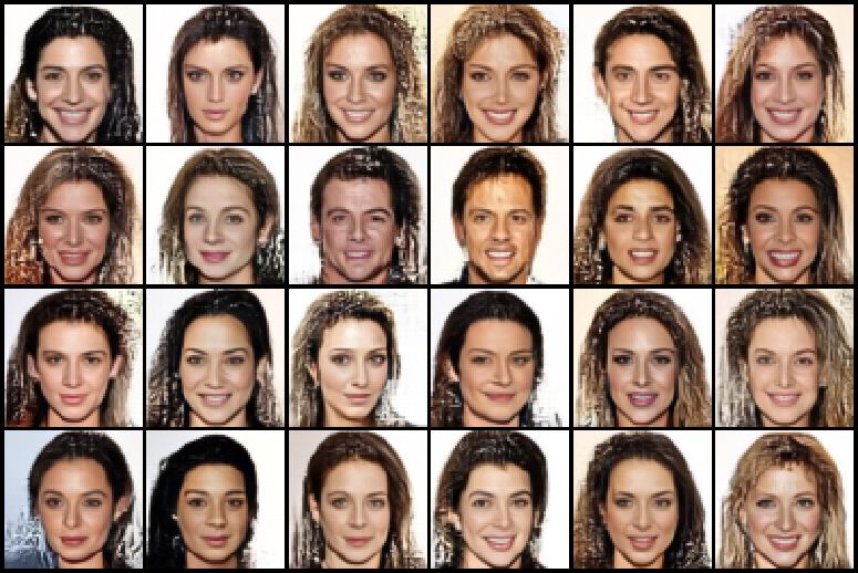
5.2 C ONDITIONAL I NFERENCE WITH C ELEBA I MAGES
Next we consider sampling a missing right half of CelebA (Liu et al., 2015) images (aligned,
cropped, and resized to 64 × 64 full color images) using a normalizing flow following the GLOW
architecture (Kingma & Dhariwal, 2018). To bolster our claim that PL-MCMC does not require spe-
cially trained models, we utilize a publicly available pre-trained model (Yuki-Chai, 2019) for this
experiment. Initial and final completions provided by the Markov Chain are illustrated in Figure 3.
(a) Initial Completions (b) Final Completions (c) Ground Truth
Figure 3: Conditional inference of CelebA images with normalizing flow trained on complete data.
The initial state of the Markov Chain is constructed by sampling from the normalizing flow at re-
duced variance. Latent space transitions are generated via small perturbations within relative co-
ordinates of the latent space. PL-MCMC is carried out for 25,000 proposals. Example progres-
sions of completions are provided in Figure 4. The progression of PL-MCMC completions clearly
demonstrates how defining a Markov Chain through the flow’s latent space encourages proposing
alterations to semantically meaningful attributes.
5
Published as a conference paper at ICLR 2021

      Figure 4: Progression of CelebA completions over intervals of 1000 PL-MCMC proposals.

5.3    C ONDITIONAL I NFERENCE WITH MNIST D IGITS

Finally, we consider sampling missing portions of MNIST (LeCun et al., 1998) digits (28 × 28
monochrome images) using a normalizing flow following a variant of the NICE architecture (Dinh
et al., 2014) under a variety of data missingness mechanisms. The missingness mechanisms consid-
ered are independent missingness (I.M.), patch missingness (P.M.), and square observation (S.O.), at
missingness rates of 0.6, 0.6, and 0.8 respectively. Final completions and conditional expectations
as obtained by averaging the final completions of 20 independent PL-MCMC chains are illustrated
in Figure 5.

          (a) Masked Inputs   (b) Final Completions (c) Conditional Means   (d) Ground Truth

Figure 5: Conditional inference of MNIST digits with normalizing flow trained on complete data.

The initial state of the Markov Chain is constructed by sampling from the normalizing flow at re-
duced variance. Latent space transitions are generated by a mixture of small perturbations within
the absolute coordinates of the latent space and resampling at reduced variance. PL-MCMC is per-
formed over 2,000 proposals. Example progressions of completions are provided in Figure 6.

      Figure 6: Progression of MNIST completions over intervals of 200 PL-MCMC proposals.

6     Q UANTITATIVE E XPERIMENTAL R ESULTS

As an analytical description of the conditional distributions of non-specialized normalizing flows is
infeasible, it is difficult to quantify how well PL-MCMC succeeds in sampling from its intended dis-
tributions. Given the extreme dependence of Algorithm 2 on accurate conditional sampling from PL-
MCMC for effective training, we therefore quantify the performance of normalizing flows trained
from incomplete data as an indication for whether PL-MCMC produces sufficiently accurate and
efficient samples to remain useful for real-world missing data tasks. We also test the sampling effi-
ciency of PL-MCMC independently of considerations regarding sampling accuracy. Further details
of these experiments are provided in Appendix E.

                                                  6
Published as a conference paper at ICLR 2021

6.1      T RAINING FROM I NCOMPLETE MNIST D IGITS

In this experiment, we consider training models of MNIST digits from training sets affected by a
variety of data missingness mechanisms and imputing test sets affected by the same missingness
mechanisms. The data missingness mechanisms used are are independent missingness (I.M.), patch
missingness (P.M.), and square observation (S.O.), with missingess rates of 0.3, 0.6, and 0.9. As
imputation performance measures, we consider per-pixel reconstruction RMSE and Fréchet Incep-
tion Distance (Heusel et al., 2017). As comparison, we include results for imputing using pixel wise
observed means and using the convolutional variant of MisGAN (Li et al., 2018). Our normalizing
flow is a variant of the NICE architecture. We performed MC-EM training of the normalizing flow
for a total of 1,000 epochs. Inference with normalizing flows is performed using a PL-MCMC chain
of 2, 000 proposals. Our reported results within Table 1 reflect performance across fifteen distinct
pairings of training and test sets (models trained, where applicable, from three distinct training sets
and each tested on five distinct test sets). For PL-MCMC, our results reflect imputation performance
using individual conditional samples (Ind.) and using the average of 10 conditional samples (Avg.)
for test set completion.

Table 1: Comparison of imputation performance for reconstructing MNIST digits. Value means are
reported to at most the first significant digit of standard error.

                      Reconstruction RMSE                                      FID
                     PL-MCMC PL-MCMC                               PL-MCMC PL-MCMC
    Rate     Mean                    MisGAN                Mean                    MisGAN
                        Ind.    Avg.                                  Ind.    Avg.
        0.3 0.2570(1) 0.153(1)    0.130(2) 0.1277(4) 23.5(1)         1.56(7)      1.58(8)     0.17(1)
 I.M.

        0.6 0.2573(1) 0.1585(6)   0.1456(1) 0.167(2) 72.2(1)         5.7(5)       6.1(5)      0.78(2)
        0.9 0.2574(0) 0.261(2)    0.256(1) 0.326(4) 114.7(1)        87(2)        90(2)       11(1)
        0.3 0.0577(3) 0.0410(3)   0.0371(3) 0.0439(6)     0.1(0)     0.075(1)     0.076(1)    0.006(1)
 S.O.

        0.6 0.1688(2) 0.152(3)    0.137(2) 0.159(2)       5.8(1)     1.4(2)       1.7(2)      0.6(1)
        0.9 0.2467(1) 0.2595(8)   0.2535(7) 0.322(1)     68.7(2)    50(2)        54(1)        4(1)
        0.3 0.2629(3) 0.1795(8)   0.1565(5) 0.1956(8) 17.0(1)        1.6(1)       1.8(1)      0.8(1)
 P.M.

        0.6 0.2641(1) 0.221(4)    0.205(3) 0.247(1)    57.6(1)      15(1)        16(1)        2.9(2)
        0.9 0.2622(0) 0.2675(8)   0.2648(9) 0.3693(9) 110.5(1)      89(2)        92(2)       16(2)

As RMSE and FID score are measures of distortion and divergence, respectively, a single imputation
estimate cannot simultaneously optimize both (Blau & Michaeli, 2018). MisGAN primarily focuses
on minimizing imputation FID, while our MC-EM training favors reducing reconstruction RMSE.
Our results highlight a potential advantage of performing imputation via sampling from conditional
distributions. With its deterministic imputation procedure, MisGAN is dedicated to minimizing FID
and cannot reduce reconstruction RMSE by averaging multiple reconstructions. With PL-MCMC
sampling, we can choose, to some degree, whether to minimize FID by imputing with a single
sample from the flow’s conditional distribution or to minimize RMSE by averaging across multiple
samples. These results demonstrate that PL-MCMC is able to sample from the conditional distri-
butions of normalizing flows sufficiently well to acceptably train normalizing flows from MNIST
digits affected by a variety of data missingness mechanisms and rates.

6.2      T RAINING FROM I NCOMPLETE UCI DATASETS

In this experiment, we consider training models of various continuous UCI datasets (Bache & Lich-
man, 2013) affected by 50% uniformly missing values. As a performance measure, we consider nor-
malized MSE of imputing missing values within the training set. As comparison, we include results
for imputing using variable-wise observed means, using the missForest (Stekhoven & Bühlmann,
2012) R package with default settings, and using VAEs via MIWAE (Mattei & Frellsen, 2019).
Our normalizing flow is a variant of the NICE architecture. We performed MC-EM training of the
normalizing flow for a total of 1,000 epochs. For inference, the PL-MCMC chain is run for 1,000
proposals. Our reported results within Table 2 reflect performance across five distinct training sets.
For PL-MCMC, our results reflect imputation performance using individual conditional samples
(Ind.) and using the average of 25 conditional samples (Avg.) for test set completion.

                                                  7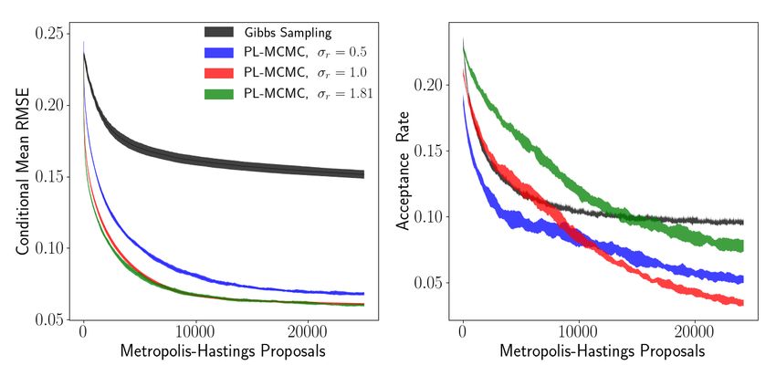
Published as a conference paper at ICLR 2021

Table 2: Comparison of imputation NMSE results for continuous UCI datasets affected by 50%
uniform missingness. Value means are reported to at most the first significant digit of standard error.

                      banknote breast concrete red-wine white-wine yeast
    PL-MCMC Ind.        1.12(5)      0.46(2)     1.22(4)       1.22(3)         1.45(3)      1.67(5)
   PL-MCMC Avg.         0.58(3)      0.31(2)     0.67(3)       0.69(3)         0.76(1)      0.96(6)
           MIWAE        0.56(4)      0.29(1)     0.63(3)       0.66(2)         0.73(3)      0.95(5)
         missForest     0.74(3)      0.31(1)     0.67(2)       0.74(3)         0.81(1)      1.18(3)
             Mean       0.99(1)      1.00(3)     1.00(1)       1.00(2)         1.01(1)      0.96(6)

In all cases, the MC-EM trained normalizing flows perform at least as well as missForest and closely
match MIWAE for estimating conditional expectations. We can conclude that, while there is some
potential room for improvement in capturing the exact ground truth conditional distributions, MC-
EM training of normalizing flows with PL-MCMC produces imputations comparable to those from
current methods for this particular task.

6.3   S AMPLING E FFICIENCY FOR I NFERENCE OF MNIST D IGIT

Here we consider the task of estimating the conditional expectation for the missing region of a single
MNIST digit using the average of 100 independent Markov Chains. We also use this experiment as
an opportunity to explore the effect on conditional sampling performance produced by different
choices for PL-MCMC’s auxiliary distribution and the transition proposal distribution. The RMSE
versus proposal number of conditional means estimated via Gibbs sampling within the modeled data
space and PL-MCMC with varying auxiliary distributions are compared in Figure 7. Statistics are
gathered from 10 distinct replications of the experiment.

Figure 7: Single standard deviation envelopes of estimated conditional mean per-pixel RMSE and
proposal acceptance rate for conditional sampling of MNIST digit. PL-MCMC implementations
only differ by choice of auxiliary density.

These results demonstrate that PL-MCMC can offer significant performance gains over comparable
MCMC methods confined to the modeled data space. Even when using an improper uniform distri-
bution as the auxiliary density (effectively omitting q from the acceptance probability calculation in
Algorithm 1), PL-MCMC can accelerate conditional sampling by leveraging the flow’s latent space
to propose more effective proposal transitions. Depending on the characteristics of the normalizing
flow’s conditional distribution, selecting a more restrictive auxiliary distribution can greatly accel-
erate sampling even further. As the results with auxiliary distributions with standard deviations of
σa = 10−3 and σa = 10−6 closely overlap, there may be some concern that the auxiliary distri-

                                                  8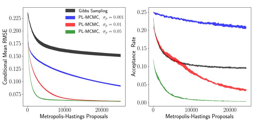
Published as a conference paper at ICLR 2021

bution might dominate PL-MCMC’s behavior and reduce the procedure to a simple search in the
latent space to best rebuild the observed data, starting around σa = 10−3 . While this concern may
be warranted when using exceedingly strong choices for the auxiliary distribution, analysis demon-
strates (Appendix E.4) that this is not the case for our results with σa = 10−3 . The RMSE versus
proposal number of conditional means estimated via Gibbs sampling within the modeled data space
and PL-MCMC with varying transition proposal distributions are compared in Figure 8.

Figure 8: Single standard deviation envelopes of estimated conditional mean per-pixel RMSE and
proposal acceptance rate for conditional sampling of MNIST digit. PL-MCMC implementations
only differ by scale of perturbations used in their transition proposals.

From these experiments, we offer a few preliminary conclusions regarding the effect of the aux-
iliary and transition proposal distributions on conditional sampling performance with PL-MCMC.
In the Metropolis-Hastings implementation of PL-MCMC, the transition proposal distribution be-
haves much as one would expect for the transition proposal distributions of any Metropolis-Hastings
procedures. Increasing the proposal distribution’s scale will accelerate initial convergence, but may
encounter problems traversing concentrated regions of the target distributions. To some target dis-
tribution dependent point (around σa = 10−1.5 in Figure 7), strengthening the auxiliary distribution
will continue to accelerate initial sampling. Beyond this point, further strengthening of the auxil-
iary distribution can be detrimental to sampling performance, as the auxiliary distribution becomes
mismatched to the intrinsic coupling between missing and observed values modeled by the flow’s
conditional distribution. Additional comparisons, including comparisons with respect to approxi-
mate computational cost, are provided within Appendix E.

7   C ONCLUSION AND F UTURE W ORK

The mathematical structure of normalizing flows is exceptionally convenient for approaching con-
ditional sampling via MCMC. By leveraging this mathematical structure, our proposed PL-MCMC
technique enables asymptotically exact conditional inference with normalizing flows, without re-
quiring specialized architecture, training history, or external inference machinery. The particular
implementations used in our experiments are primarily intended to serve as proof-of-concept illus-
trations of the PL-MCMC technique. Further research would be necessary to determine optimal
choices of auxiliary distributions,transition proposal distributions, and MC-EM training procedures.
Sampling performance may be improved by replacing Metropolis-Hastings proposals with a more
sophisticated technique, such as Hamiltonian Monte Carlo. Our experimental results demonstrate
that, even when implemented with a naive Metropolis-Hastings procedure, PL-MCMC enables ef-
fective sampling from its intended distributions under practical settings. We believe that, with the
PL-MCMC technique, normalizing flows hold great promise for approaching missing data tasks.

                                                 9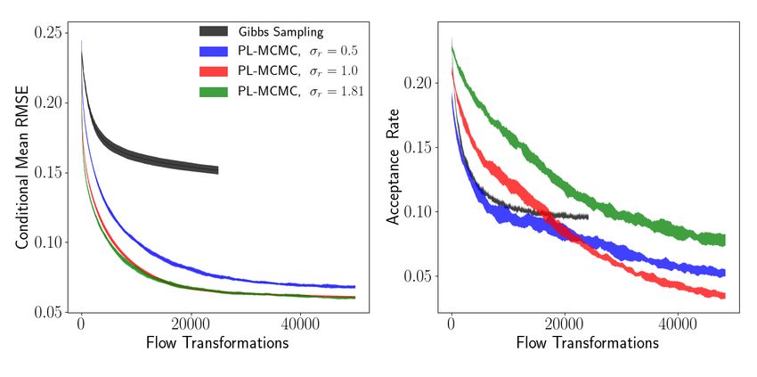
Published as a conference paper at ICLR 2021

ACKNOWLEDGEMENTS
This work was supported by the Office of Naval Research Grant No. N00014-18-1-2244.

R EFERENCES
Kevin Bache and Moshe Lichman. UCI Machine Learning Repository, 2013.
Yochai Blau and Tomer Michaeli. The Perception-Distortion Tradeoff. In Proceedings of the IEEE
  Conference on Computer Vision and Pattern Recognition, pp. 6228–6237, 2018.
Arthur P Dempster, Nan M Laird, and Donald B Rubin. Maximum Likelihood from Incomplete
  Data Via the EM Algorithm. Journal of the Royal Statistical Society: Series B (Methodological),
  39(1):1–22, 1977.
Laurent Dinh, David Krueger, and Yoshua Bengio. NICE: Non-linear Independent Components
  Estimation. arXiv preprint arXiv:1410.8516, 2014.
Alain Durmus, Eric Moulines, et al. High-dimensional Bayesian Inference Via the Unadjusted
  Langevin Algorithm. Bernoulli, 25(4A):2854–2882, 2019.
Daniel Foreman-Mackey, David W Hogg, Dustin Lang, and Jonathan Goodman. EMCEE: The
  MCMC Hammer. Publications of the Astronomical Society of the Pacific, 125(925):306, 2013.
Glenn Fredrickson et al. The Equilibrium Theory of Inhomogeneous Polymers, volume 134. Oxford
  University Press on Demand, 2006.
Matthew M Graham, Amos J Storkey, et al. Asymptotically Exact Inference in Differentiable Gen-
 erative Models. Electronic Journal of Statistics, 11(2):5105–5164, 2017.
Ulf Grenander and Michael I Miller. Representations of Knowledge in Complex Systems. Journal
  of the Royal Statistical Society: Series B (Methodological), 56(4):549–581, 1994.
Heikki Haario, Eero Saksman, Johanna Tamminen, et al. An Adaptive Metropolis Algorithm.
  Bernoulli, 7(2):223–242, 2001.
Martin Heusel, Hubert Ramsauer, Thomas Unterthiner, Bernhard Nessler, and Sepp Hochreiter.
 GANs Trained by a Two Time-Scale Update Rule Converge to a Local Nash Equilibrium. In
 Advances in Neural Information Processing Systems, pp. 6626–6637, 2017.
Matthew Hoffman, Pavel Sountsov, Joshua V Dillon, Ian Langmore, Dustin Tran, and Srinivas
 Vasudevan. Neutra-lizing Bad Geometry in Hamiltonian Monte Carlo using Neural Transport.
 arXiv preprint arXiv:1903.03704, 2019.
Oleg Ivanov, Michael Figurnov, and Dmitry Vetrov. Variational Autoencoder with Arbitrary Condi-
  tioning. arXiv preprint arXiv:1806.02382, 2018.
Durk P Kingma and Prafulla Dhariwal. Glow: Generative Flow with Invertible 1x1 Convolutions.
  In Advances in Neural Information Processing Systems, pp. 10215–10224, 2018.
Alex Krizhevsky et al. Learning Multiple Layers of Features from Tiny Images. 2009.
Yann LeCun, Léon Bottou, Yoshua Bengio, and Patrick Haffner. Gradient-based Learning Applied
  to Document Recognition. Proceedings of the IEEE, 86(11):2278–2324, 1998.
Steven Cheng-Xian Li. misgan. https://github.com/steveli/misgan, 2019.
Steven Cheng-Xian Li, Bo Jiang, and Benjamin Marlin. MisGAN: Learning from Incomplete Data
  with Generative Adversarial Networks. In International Conference on Learning Representations,
  2018.
Yang Li, Shoaib Akbar, and Junier B Oliva. Flow Models for Arbitrary Conditional Likelihoods.
  arXiv preprint arXiv:1909.06319, 2019.

                                               10
Published as a conference paper at ICLR 2021
Roderick JA Little and Donald B Rubin. Statistical Analysis with Missing Data, volume 793. John
Wiley & Sons, 2019.
Ziwei Liu, Ping Luo, Xiaogang Wang, and Xiaoou Tang. Deep Learning Face Attributes in the Wild.
In Proceedings of the IEEE International Conference on Computer Vision, pp. 3730–3738, 2015.
You Lu and Bert Huang. Structured Output Learning with Conditional Generative Flows. In AAAI,
pp. 5005–5012, 2020.
P.A. Mattei. miwae. https://github.com/pamattei/miwae, 2019.
Pierre-Alexandre Mattei and Jes Frellsen. Leveraging the Exact Likelihood of Deep Latent Variable
Models. In Advances in Neural Information Processing Systems, pp. 3855–3866, 2018.
Pierre-Alexandre Mattei and Jes Frellsen. MIWAE: Deep Generative Modelling and Imputation of
Incomplete Data Sets. In International Conference on Machine Learning, pp. 4413–4423, 2019.
Fengzhou Mu. Nice. https://github.com/fmu2/NICE, 2019.
Thomas Müller, Brian McWilliams, Fabrice Rousselle, Markus Gross, and Jan Novák. Neural Im-
portance Sampling. ACM Transactions on Graphics (TOG), 38(5):1–19, 2019.
Ronald C Neath et al. On Convergence Properties of the Monte Carlo EM Algorithm. In Advances
in Modern Statistical Theory and Applications: a Festschrift in Honor of Morris L. Eaton, pp.
43–62. Institute of Mathematical Statistics, 2013.
Danilo Jimenez Rezende, Shakir Mohamed, and Daan Wierstra. Stochastic Backpropagation and
Approximate Inference in Deep Generative Models. In International Conference on Machine
Learning, pp. 1278–1286, 2014.
Trevor W Richardson, Wencheng Wu, Lei Lin, Beilei Xu, and Edgar A Bernal. MCFlow: Monte
Carlo Flow Models for Data Imputation. In Proceedings of the IEEE/CVF Conference on Com-
puter Vision and Pattern Recognition, pp. 14205–14214, 2020.
Daniel J Stekhoven and Peter Bühlmann. MissForest—Non-parametric Missing Value Imputation
for Mixed-type Data. Bioinformatics, 28(1):112–118, 2012.
Dimiter Tsvetkov, Lyubomir Hristov, and Ralitsa Angelova-Slavova. On the Convergence of the
Metropolis-Hastings Markov Chains. arXiv preprint arXiv:1302.0654, 2013.
Joost van Amersfoort. Glow-pytorch. https://github.com/y0ast/Glow-PyTorch,
2019.
David A Van Dyk. Marginal Markov Chain Monte Carlo Methods. Statistica Sinica, pp. 1423–1454,
2010.
Greg CG Wei and Martin A Tanner. A Monte Carlo Implementation of the EM Algorithm and the
Poor Man’s Data Augmentation Algorithms. Journal of the American Statistical Association, 85
(411):699–704, 1990.
Jinsung Yoon, James Jordon, and Mihaela Van Der Schaar. GAIN: Missing Data Imputation using
Generative Adversarial Nets. arXiv preprint arXiv:1806.02920, 2018.
Yuki-Chai. glow-pytorch. https://github.com/chaiyujin/glow-pytorch, 2019.
Michael Zhu. Sample Adaptive MCMC. In Advances in Neural Information Processing Systems,
pp. 9066–9077, 2019.
11Published as a conference paper at ICLR 2021
A K NOWING THE J OINT D ISTRIBUTION I MPLIES K NOWING THE
C ONDITIONAL D ISTRIBUTIONS
In this section, we establish a fundamental guarantee regarding the accuracy of the conditional dis-
tributions known by generative models. Consider two random variables, x and y, with ground truth
joint distribution px,y that we have approximated by a generative model with joint distribution qx,y .
In the discrete case, we may expand through the definition of the Kullback-Liebler divergence be-
tween our generative model and the ground truth to find that:
X X
DKL (px,y ||qx,y ) = − p(x, y) log q(x, y) + p(x, y) log p(x, y)
x,y x,y
X X
= Ex [− p(y|x) log q(y|x)q(x) + p(y|x) log p(y|x)p(x)]
y y
= Ex [DKL (py|x ||qy|x ) − log q(x) + log p(x)]
= Ex [DKL (py|x ||qy|x )] + DKL (px ||qx ).
From the non-negativity of the Kullback-Liebler divergence, we are then guaranteed:
DKL (px,y ||qx,y ) ≥ Ex [DKL (py|x ||qy|x )].
With equality only when our generative model perfectly models the marginal distribution of x. When
considering the task of inferring y from observed values of x, the expected performance of our
generative model in approximating the conditional distribution of y given x is no worse than its
performance in approximating the full joint distribution between x and y. Therefore, if we know that
a generative model is a good approximation of the joint distribution governing some set of random
variables, then it must also know good approximations of the conditional distributions among those
random variables.
This inequality also serves as a justification for Monte Carlo Expectation Maximization training.
When using our modeled distribution qx,y to impute an incomplete training set, the newly imputed
training set is sampled from the distribution qy|x px . We can easily see that:
DKL (px,y ||qy|x px ) = Ex [DKL (py|x ||qy|x )] ≤ DKL (px,y ||qx,y ).
In the asymptotic limit of dataset size, conditionally inferring missing values within the dataset
results in samples from a distribution whose divergence from ground truth is no worse than that
of the original model. Assuming that the original model describes the distribution of a previously
imputed version of the training set, this implies that our newly training set is at least as reflective
of the ground truth distribution as the previous training set. In practice, we find that conditional
imputation tends to improve divergence of the training set, which in turn allows MC-EM training to
improve our model of the joint distribution.
B T HE A DVANTAGE OF L ATENT S PACE P ROPOSALS
Here, we relay our intuition regarding the advantages of defining a Markov Chain within the latent
space of a normalizing flow. This section provides a heuristic argument and therefore utilizes infor-
mal terminology to convey our current understanding. Take a normalizing flow between latent space
Ξ and modeled data space X , defining the mappings fθ : Ξ 7→ X and fθ−1 : X 7→ Ξ. This normal-
izing flow imposes the probability density pf,θ (x) onto all modeled data values x ∈ X . As practical
applications of normalizing flows primarily involve data embedded within a euclidean space, we
will confine this discussion to scenarios where latent and modeled data values are both points in Rn
for some n. In these cases, it is straightforward to discuss neighborhoods of fixed radius around
points within both the latent and modeled data spaces.
For now, let us consider the task of forming a Markov Chain for unconditionally sampling from
the density pf,θ (x). For simplicity, let us only consider proposal perturbations within some fixed
12Published as a conference paper at ICLR 2021
radius of the Markov Chain’s current state. With the one-to-one mapping provided by the flow,
we have the option of tracking and perturbing the current state within either the latent space or the
modeled data space. When considering the neighborhood of data points, probability mass within
the modeled data space is often non-isotropic for highly structured data. However, probability mass
is nearly isotropic within the latent space in the neighborhood of the latent representations of data
points, assuming that the distribution on latent space states has been appropriately chosen (as is the
case for the commonly used multivariate normal or logistic distributions). As a result, performing
an isotropic perturbation within the latent space results in proposals that are about as likely as the
starting state. Within the modeled data space, even a very small isotropic perturbation can produce
proposals that are far more unlikely than the starting state. As an example, suppose our normalizing
flow was well trained to model a set of high-fidelity images. If our proposals within the modeled data
space were created by adding independent Gaussian perturbations to pixel values, we would almost
always inject noise into the image and proposals within the modeled data space would be tend to be
unlikely, low-fidelity images. With the assumption that transitions between equally likely states are
usually accepted and transitions to much more unlikely states are usually rejected, we should expect
latent space proposals to be accepted more frequently compared to modeled data space proposals.
As an intuition, we could say that perturbations within the flow’s latent space are semantically mean-
ingful for the modeled data set. As demonstrated by Hoffman et al. (2019), the normalizing flow
inherently transforms the modeled probability distribution in a manner that is well suited to explo-
ration using naive, isotropic proposals. This is related to Adaptive Monte Carlo methods (Haario
et al., 2001; Foreman-Mackey et al., 2013; Zhu, 2019), which attempt to transform the proposal
density to most effectively explore a fixed distribution. With latent space transitions in normalizing
flows, it is as though the modeled data distribution has been transformed so as to be best explored
by a fixed proposal density.
With PL-MCMC we are concerned with making effective proposals with respect to a conditional
distribution. Even when attempting to sample a conditional distribution, utilizing latent space pro-
posals remains beneficial. Define a projection operator via projxO (yM ; yO ) = yM ; xO , which
simply replaces the observed component of a y ∈ X with the conditioning values xO . The elements
of a proposed transition within a Metropolis-Hastings implementation of PL-MCMC are illustrated
in Figure 9.
Figure 9: A Metropolis-Hastings PL-MCMC proposal when inferring from observed data xO .
Averaging over possible pieces of observed data xO , we expect to find that the set of likely com-
pletions, xM , under the conditional density pf,θ (xM |xO ) remains essentially a subset of the set
13Published as a conference paper at ICLR 2021
of likely values under the marginalized density pf,θ (xM ). If a proposed xM is unlikely under
pf,θ (xM ), we expect it to be unlikely under pf,θ (xM |xO ). Hence, with PL-MCMC, the advantages
of latent space proposals carry through to the conditional inference setting, as the resulting proposed
completions can remain likely under pf,θ (xM ).
Returning to the example of modeling a set of high-fidelity images, suppose we observe the left half
of these images. In general, we would believe that the set of likely right half completions conditioned
on the observed left half is well covered by set of likely right halves that we see across the entire
distribution of images. Perturbing the pixel values of the right half injects noise, tending to produce
a low-fidelity right half, which results in an unlikely, noisy image when combined with the observed
left half. Following the PL-MCMC latent perturbations, proposed right halves may be more able to
at least remain the high-fidelity right halves of high-fidelity images.
By employing latent space proposals to sample from pf,θ (xM |xO ), PL-MCMC can more easily
propose completions xM that could plausibly have been taken from likely members of the modeled
data distribution. Of course, for conditional inference, we also need to produce samples that are well
matched to the observed data. While latent space proposals assist in making meaningful and efficient
transitions within a Markov Chain, PL-MCMC ultimately relies on the auxiliary distribution, q, and
guaranteed convergence to the correct conditional distribution to effectively sample from typical
completions of the observed data.
C D ETAILS OF MC-EM T RAINING
In this section we review the derivation of Monte Carlo Expectation maximization (Dempster et al.,
1977; Wei & Tanner, 1990; Neath et al., 2013) in the context of its use with PL-MCMC. Suppose we
are presented with a training set of T observed values (not all missing the same entries), Xtrain =
{xO,1 , xO,2 , . . . , xO,T }. Ideally, under the assumption that data values are missing at random (Little
& Rubin, 2019), we’d wish to find the flow parameters θ that maximize the log-likelihood of Xtrain :
XT Z
log pf,θ (Xtrain ) = log pf,θ (xM,i ; xO,i )dxM,i .
i=1 xM,i
Yet the complexity of the normalizing flow makes an analytical computation of the marginal like-
lihoods of observed data entirely impractical. We therefore utilize the Expecation-Maximization
(EM) algorithm (Dempster et al., 1977) to approach this optimization. Following Dempster et al.
(1977), we define Q(θ0 |θ) to be:
T
X
Q(θ0 |θ) = Epf,θ [log( pf,θ0 (xM,i ; xO,i ) )| xO,i ].
i=1
PL-MCMC can be immediately applied to approximate these expectations. Let the set Y =
{yM,1 , yM,2 , . . . , yM,T } be created by sampling each yM,i ∼ pf,θ (yM,i |xO,i ) using a PL-MCMC
chain as described previously. We may now use the approximation:
T
X
Q(θ0 |θ) ≈ log( pf,θ0 (yM,i ; xO,i ) ).
i=1
In principle, we would then update θ following;
θ ← argmax Q(θ0 |θ).
θ0
In practice, it is more feasible to continue to train the flow on the conditionally imputed version of
0
Xtrain . With Xtrain = {(yM,1 ; xO,1 ), (yM,2 ; xO,2 ), . . . , (yM,T ; xO,T )} denoting our newly im-
puted training set and train being any training procedure that returns flow parameters θ approx-
imately maximizing the likelihood of a complete data training set, we rely on the approximation
that:
14Published as a conference paper at ICLR 2021
argmax Q(θ0 |θ) ≈ train(f, Xtrain
0
).
θ0
This approximation immediately leads to our described algorithm for the MC-EM training of nor-
malizing flows using PL-MCMC.
D D ETAILS R EGARDING Q UALITATIVE E XPERIMENTS
D.1 D ETAILS R EGARDING C ONDITIONAL I NFERENCE WITH CIFAR-10 I MAGES
In this experiment, we infer a missing central quarter (an 8 × 8 pixel square) of CIFAR-10
(Krizhevsky et al., 2009) images. The CIFAR-10 dataset is composed of 60, 000 full color 32 × 32
images of 10 distinct classes of objects, with 6, 000 images provided for each class. The standard
training and test set split for the CIFAR-10 dataset is 50, 000 and 10, 000 images, respectively.
Our chosen normalizing flow is a variant of the GLOW (Kingma & Dhariwal, 2018) architecture.
We utilized a publicly available, pre-trained model (van Amersfoort, 2019) for this experiment. In
the terminology of Kingma & Dhariwal (2018), the model has a depth of flow (K) of 32 and a total
of 3 levels (L) and flow layers utilize 512 hidden channels. The model was reportedly trained for
a total of 1, 500 epochs using Adamax with a learning rate of 5 × 10⁻⁴ and a batchsize of 64. We
presume, but cannot guarantee, that the model was trained on the standard 50, 000 example CIFAR-
10 training set. Examples of unconditioned samples from this model are provided within Figure 10,
as obtained with the standard sampling variance, σ = 1.0 (temperature T = 1.0, in the terminology
of Kingma & Dhariwal (2018)). From these unconditioned samples, it is clear that the model has
not collapsed to memorizing the training set.
Figure 10: Unconditioned samples at standard variance (σ = 1.0) from CIFAR-10 model.
The particular implementation of the normalizing flow most easily provided access to a coordinate
dependent representation of the latent space, which we call absolute coordinates for the latent space.
Fundamentally, the Markov Chain within PL-MCMC may utilize any convenient representation of
the latent space, so long as a diffeomorphism still maps that representation back to the modeled
data. For this CIFAR-10 experiment, we chose to employ a Markov Chain within the architecture’s
absolute coordinates. As a general note, the qualifier “absolute” merely refers to the representation
favored by the flow’s implementation, while the qualifier “relative” refers to the representation best
coinciding with the chosen prior distribution for the flow. The terms only reflect aspects of our prac-
15Published as a conference paper at ICLR 2021
tical usage of the representations, as there is no theoretically favored diffeomorphic representation
of the latent space.
For inference, we selected images from the standard CIFAR-10 test set. During inference with
PL-MCMC, latent space transitions are generated within the above mentioned absolute coordinates
of the flow’s latent space by small perturbations from the current latent state. When perturbing
the latent state, proposals are generated following a perturbation kernel, gp (ξ 0 |ξ), such that ξ 0 ∼
N (ξ, σp2 I). The auxiliary distribution, q, is chosen to target yO ∼ N (xO , σa2 I). For this experiment,
we select σp = 0.01 and σa = 1 × 10⁻³ . PL-MCMC is carried out over 25,000 proposals.
D.2 D ETAILS R EGARDING C ONDITIONAL I NFERENCE WITH C ELEBA I MAGES
In this experiment, we infer a missing right half (a 64 × 32 pixel rectangle) of CelebA (Liu et al.,
2015) images. The CelebA dataset is composed of 202, 599 full color images of celebrity faces. We
utilize the aligned and cropped version of the CelebA dataset, resized to a size of 64 × 64.
Our chosen normalizing flow is a variant of the GLOW (Kingma & Dhariwal, 2018) architecture.
We utilized a publicly available, pre-trained model (Yuki-Chai, 2019) for this experiment. In the
terminology of Kingma & Dhariwal (2018), the model has a depth of flow (K) of 32 and a total of
3 levels (L) and flow layers utilize 512 hidden channels. The model was reportedly trained for a
total of 1, 500 epochs using Adamax with a learning rate of 1 × 10⁻³ and a batchsize of 12. We
believe that this model was trained on the entirety of the CelebA dataset, with no withheld test or
validation set. Examples of unconditioned samples from this model are provided within Figures 11
and 12, as obtained with reduced and standard sampling variance, σ = 0.5 and σ = 1.0 respectively
(temperatures T = 0.5 and T = 1.0, in the terminology of Kingma & Dhariwal (2018)). From these
unconditioned samples, it is clear that the model has not collapsed to memorizing the training set.
Figure 11: Unconditioned samples at reduced variance (σ = 0.5) from CelebA model.
16Published as a conference paper at ICLR 2021
Figure 12: Unconditioned samples at standard variance (σ = 1.0) from CelebA model.
As in the CIFAR-10 experiment, the particular implementation of the normalizing flow most eas-
ily provided access to a coordinate dependent representation of the latent space, which we call
absolute coordinates for the latent space. For this CelebA experiment, we chose to employ a
Markov Chain within what we call relative coordinates of the latent space. For this architecture,
we have convenient access to three subsets of latent variables, ξ1 , ξ2 , and ξ3 within absolute coor-
dinates. Fixing ξ1 (resp. fixing ξ1 and ξ2 ) there is an invertible transformation h2 (ξ2 ; ξ1 ) (resp.
h3 (ξ3 ; ξ1 , ξ2 )) such that h2 (ξ2 ; ξ1 ) ∼ N (0, I) (resp. h3 (ξ3 ; ξ1 , ξ2 ) ∼ N (0, I)) under our flow’s
prior. The Markov Chain in relative coordinates simply follows and proposes transitions for the
triplet (ξ1 , h2 (ξ2 ; ξ1 ), h3 (ξ3 ; ξ1 , ξ2 )).
As it appears that no test set had been withheld during training of the model, we selected images
at random from the full dataset for our experiment. During inference with PL-MCMC, latent space
transitions are generated within relative coordinates of the flow’s latent space by small perturbations
from the current latent state. When perturbing the latent state, proposals are generated following a
perturbation kernel, gp (ξ 0 |ξ), such that ξ 0 ∼ N (ξ, σp2 I). The auxiliary distribution, q, is chosen to
target yO ∼ N (xO , σa2 I). For this experiment, we select σp = 0.01 and σa = 1×10⁻³ . PL-MCMC
is carried out over 25,000 proposals.
D.3 D ETAILS R EGARDING C ONDITIONAL I NFERENCE WITH MNIST D IGITS
In this experiment, we infer missing portions of MNIST (LeCun et al., 1998) digits. The MNIST
dataset is composed of 70, 000 monochrome 28 × 28 images of handwritten digits. The standard
training and test set split for the MNIST dataset is 60, 000 and 10, 000 images, respectively. Our data
missingness mechanisms are independent missingness, where pixels are lost uniformly at random,
patch missingness, where randomly located contiguous rectangular blocks are missing, and square
observation, where only a randomly located contiguous square is observed.
Our chosen normalizing flow is a variant of the NICE (Dinh et al., 2014) architecture. Our im-
plementation is a modification of that by Mu (2019). In the terminology of Kingma & Dhariwal
(2018), the model has a depth of flow (K) of 5 and a total of 4 levels (L) and intermediate flow
layers have a dimension of 1000. The flow utilizes an independent logistic prior distribution. Rather
than splitting even and odd pixels within coupling layers, we split between two randomly selected
partitions that are chosen at the time of the flow’s initialization and remain fixed for all layers of
the flow. Of course, better performance would be expected by selecting a flow architecture that best
17Published as a conference paper at ICLR 2021
suits the spatial organization of image data. However, random partitioning ensures that the expected
performance of the flow remains independent of the spatial structuring of the data.
The normalizing flow is trained for 1000 epochs over the standard 60, 000 element MNIST training
set using RMSprop with a learning rate of 1 × 10⁻⁵ and a momentum of 0.9 and a batch size of 200.
The data is pre-processed by performing pixel-wise whitening of the dataset (subtracting pixel-wise
observed means and dividing by pixel-wise observed standard deviation). The training procedure is
intended to follow that used later for training from incomplete MNIST digits to serve as a baseline
for comparison and is not intended to produce the best possible generative model of MNIST digits.
Examples of unconditioned samples from this model are provided within Figure 13, as obtained with
the standard sampling variance (temperature T = 1.0, in the terminology of Kingma & Dhariwal
(2018))
Figure 13: Unconditioned samples at standard variance from MNIST model.
During inference with PL-MCMC, latent space transitions are generated within the absolute co-
ordinates of the flow’s latent space, half of the time at random by small perturbations from the
current latent state and half of the time entirely resampled at a reduced standard deviation. When
perturbing the latent state, proposals are generated following a perturbation kernel, gp (ξ 0 |ξ), such
that ξ 0 ∼ N (ξ, σp2 I). When completely resampling the latent state, proposals are generated fol-
lowing a resampling kernel, gr (ξ 0 |ξ), such that ξ 0 ∼ N (0, σr2 I). The auxiliary distribution, q, is
chosen to target yO ∼ N (xO , σa2 I). For this experiment, we select σp = 0.05, σr = 0.5, and
σa = 1 × 10⁻³ . To simplify calculation of Metropolis-Hastings acceptance probabilities, we em-
ploy the assumption that small displacements in the latent space result from gp (ξ 0 |ξ) while large
displacements result from gr (ξ 0 |ξ), which is valid in the limit of σpYou can also read